Human Capital Composition, Growth and
Development in an R&D Endogenous Growth
Model
∗ Tiago Neves Sequeira†Abstract
The effect of human capital composition on growth and develop-ment has been somewhat neglected in economic literature. However, evidence has suggested the importance of engineering and technical skills to economic growth and international organizations had sug-gested their shortage in developed countries. Using a standard increas-ing variety endogenous growth model, we propose various measures of this composition. We show that human capital composition matters to growth and development, that the decentralized equilibrium leads to less investment in high-techs than the optimum and that the tendency to under-invest in R&D is expanded when human capital composition
∗I am grateful to the Funda¸c˜ao para a Ciˆencia e Tecnologia for financial support during
the second year of my Ph.D. program (PRAXIS XXI / BD / 21485 / 99). I am grateful to my advisors Ana Balc˜ao Reis and Jos´e Tavares for extensive discussion and suggestions and to John Huffstot for text revision. I also gratefully acknowledge participants of the Informal Research Workshop at the Faculdade de Economia, Universidade Nova de Lisboa, Research Seminar at Escola de Economia e Gest˜ao, Universidade do Minho and XXVII
Simposio de Analisis Economico, Salamanca and Carlos Os´orio for discussion and many
comments and suggestions. This paper has circulated in a previous version under the title “Human Capital, Growth and Development: an old Theory and a new Puzzle”. The usual disclaimer applies.
†Doctoral candidate at Faculdade de Economia, Universidade Nova de Lisboa, and
Teaching assistant at Departamento de Gest˜ao e Economia, Universidade da Beira
is considered. When compared to data, the model does well in explain-ing the rate of growth and the level of development (less robustly) as a function of these measures.
JEL Classification: O15, O33.
Key-Words: Human Capital Composition, Growth, Development, R&D.
1
Introduction
The effects of general human capital on growth has been widely studied in the economic literature. In Romer (1990), human capital is the key input to the research sector, which generates the new products or ideas that underlie technological progress. This means that countries with a larger stock of human capital tend to grow faster. In multicountry models of technological change the spread of new ideas across countries (or firms or industries) is also important. As Nelson and Phelps (1966) suggested, a larger stock of human capital makes it easier for a country to absorb the new products and ideas that have been discovered elsewhere and the introduction of human capital qualifies the scale-effect of population (Temple and Voth, 1998). Therefore, a follower country with more human capital tends to grow faster than others with less human capital because it catches up more rapidly to the technological leader. When studying a cross-section of countries, Barro (1991) concluded that for a given starting point of per capita GDP, a country’s subsequent growth rate is positively related to school-enrollment rates, as a proxy of human capital.
Becker, Murphy and Tamura (1990) assume that the rate of return on human capital increases over some range, an effect that could arise because of the spillover benefits from human capital that Lucas (1988) stressed.
Nevertheless, the effects of human capital composition on growth and development is a more recent field in the economic literature. The idea that
some types of human capital contribute more to growth than others do is intuitive, mainly if we think about R&D models in the spirit of Romer (1990) or Grossman and Helpman (1991), because there are only certain types of human capital engaged in R&D activities.
The first paper in this class was the one from Murphy, Shleifer and Vishny (1991), which supports the idea that the allocation of talent is im-portant for growth and bases the argument on the choice between being en-trepreneur or rent-seeker. They argue that rent-seeking rewards talent more than entrepreneurship. They proxied rent-seeking by the proportion of Law students in colleges and entrepreneurship by the proportion of Engineering students in colleges and show some evidence that the second contribute to growth while the first do not.
With special concern for growth and development (defined as GDP per
capita), Bertocchi and Spagat (1998) explain the evolution of the ratio
be-tween vocational and general education at the secondary level using social stratification and political participation. They show that this ratio is pos-itively correlated with GDP for poor countries and negatively correlated for wealthier countries. Iyigun and Owen (1999) examine the implications for growth and development of the existence of two types of human capi-tal: entrepreneurs and professionals. The first accumulates human capital through work experience and the latter through schooling. The return of en-trepreneurship is uncertain. The conclusion is that as technology improves, individuals devote less time to accumulation of human capital through work experience and more time through education, which is also supported by data. Barro (1999) used data on students’ scores on comparable interna-tional examinations on a growth regression and shows that scores on sci-ences and mathematics had a positive relationship with economic growth, but scores on the reading test were insignificantly related to growth. Also Crafts (1995), in a well-known survey performing to the British Industrial
Revolution, showed some aspects of the allocation of talent in England in which he shows that Lawyers as a percentage of occupied population have steadily decreased between 1688 and 1871 and the ratios between Engineers and Lawyers and Engineers and Accountants sharply increased between 1841 and 1881. A comparison between the development process of Mexico and USA, in the colonial period, supports the belief that “the British colonies had a better educated population, greater intellectual freedom and social mobility. Education was secular with emphasis on pragmatic skills and yan-kee ingenuity (...). The 13 British colonies had nine universities in 1776 for 2.5 million people. New Spain, with 5 million, had only two universities in Mexico City and Guadalajara, which concentrated on theology and law.” (Maddison, 2001).
A recent range of literature has been considering human capital compo-sition in somewhat different environments. Acemoglu (2001) shows microe-conomic evidence on relations between some professions and the stream of wages. As an example, Engineers and computer science jobs explain pos-itively the variations on wages, while Natural Science, Medical and Law occupations (among others) tend to have a negative coefficient from wage regression.
This all seems to suggest that allocation of human capital matters in economic growth.
Until now, no one has addressed the question of allocation of talent in an R&D-model environment.1 We will base our argument on the role of Human
Capital in R&D activities and will account for the relationship between these professionals and growth. In empirical terms we will focus on composition of Human Capital from tertiary education (Colleges and Universities). On the classification of professions, OECD and UNESCO support the belief that
1It should be stressed that this kind of model could easily account for technological
adoption. It is sufficient to consider a sector for adoption or imitation of technology instead or simultaneously with a sector of creation of new varieties or qualities.
the main labor input on R&D labs are scientists and engineers and its ratio to total human capital is usually used as an R&D indicator for cross-country comparisons.
There is a strong belief that wealthier countries invest more in R&D activities2 than do poor and middle income countries. However, recent evi-dence from European Commission (1999) and OECD (2001) showed a rela-tive shortage of engineering and technical skills in the developed countries. In Europe “more than a quarter of the graduates of colleges and universities are from social sciences” (European Commission, 1999). We also address the relationship between a measure of Human Capital composition and the level of development of a country.3
In Section 1.1, we carefully define high-tech and low-tech human capital. In Section 2 we present a model that extends Grossman and Helpman (1991) to the inclusion of human capital composition and treat endogenously the choice between different types of human capital. The model also accounts for different allocations of human capital throughout sectors in the economy. First, we describe the supply-side of the labour market equilibrium and derive an equibrium condition for the wage ratio. This is the crucial part of the model. Then, measures of high-tech intensity and the equilibrium relationships between these measures and economic growth and development are obtainned. We compare the decentralized equilibrium with the social planner solution. In Section 3, we present some evidence that supports our model, testing the relationship between measures of high-tech proportion and high-tech stock and economic growth and development.
2And then in human capital dedicated to R&D, which are mainly from technical and
engineering fields.
3Development is measured by GDP per capita. This is, of course, a restrictive measure
1.1 Defining Human capital composition as high-techs ver-sus low-techs
Generally, High-Tech human capital is defined as the stock of technical and engineering skills in the economy. Thus, High-Tech proportion is the propor-tion of this stock in total human capital. Low-tech human capital is defined as social and organizational skills. Empirically, due to lack of disaggregated data for total human capital, we use tertiary education data from the UN-ESCO dataset (see section 3 for details) and we divide high-tech human capital from all the other types (which we define as low-tech).
Definition 1 Empirically, we define high-tech human capital as the
enroll-ments in “Engineering” and “Mathematics and computer science” fields in the tertiary education level. High-tech proportion is the ratio of high-tech human capital in total enrollment in tertiary education level.
These data suggests that the allocation of different types of human cap-ital is different across sectors. For instance correlations between the em-ployment share in industry and the proportion of engineering and technical skills are near 40% while correlations between the employment share in ser-vices/agriculture and the engineering and technical proportion are near 20% and -30%, respectively. Correlations between the same measure of high-tech proportions and added values shares follow the same tendency. The follow-ing table summarizes these results.
Table 1 - Correlations between high-tech proportion and Sectors’ shares Male Workforce Female Workforce Added Values
Agriculture -29% -29% -26%
Industry 40% 41% 26%
Services 20% 14% 9%
2
The Model
This section describes the model used in the paper which extends Grossman and Helpman (1991, Chapter 3 and Chapter 5.2) to the consideration of two types of human capital.
We assume that the economy is populated with a continuum of agents. Each agent lives for a time interval of finite length T. The age distribution is uniform at every moment, with a density of N/T individuals of every age between 0 and T. At each instant the individuals who die (those who reach age T) are replaced in the population by an equal number of newborns. Therefore, the total population has constant measure N.
At every instant, each agent must allocate his or her time to one of three activities. The individual may choose to take employment as low-tech, to take employment as high-tech or to spend the time accumulating human capital. When one chooses the second option he must spend more time in the educational system and spend more money in training than when he chooses the first. We assume that the time spent in educational programs by high tech workers is fixed, exogenous and equal to S.4
Low-tech types work in the homogeneous goods sector (which we call Z) and high-tech types work in the differentiated goods sector (D) and in research labs. This follows the evidence on the allocation of different types of human capital among sectors in the economy (see Table 1). However, the crucial assumption here is that R&D is high-tech intensive.
We also make the assumption that all individuals are alike in their ca-pacity for learning5.
4This quantity of time S may be interpreted as the difference between the time spent
at school by high-tech workers and by low-tech workers. For simplicity, we neglect the time someone spends at college when he makes the low-tech choice and we also neglect all inputs other than the time devoted by the individual pupil.
5As we will analyze data in a cross section of countries, it is not clear that we should
2.1 Labor market - supply side
In the first stage of the model individuals decide whether to be high-tech or low-tech workers. This is the supply side of the labor market equilibrium. In the second stage, supply of H and L are defined and market-clearing con-ditions may be written to each of the stocks created in the early stage. With this, we make stocks of high-tech and low-tech human capital endogenous.
We first model the discrete decision of becoming a high-tech worker or a low-tech one. It follows that an individual facing this decision must compare the present value of lifetime earnings as a low-tech worker
Z t+T
t
e−ρ(τ −t)wLdτ = 1ρ(1 − e−ρT)wL (1)
with the present value of the income that the individual would obtain by spending the first S years in high-tech educational programs and supporting a private entry cost δ. For simplicity, we assume that this cost decreases gross wage in all periods after the first S, although the cost may be supported only in the S first years. This is an assumption of borrowing for education.6
The present value of these latter streams equals Z t+T t+S e−ρ(τ −t)wH δ dτ = 1 ρ(e −ρS− e−ρT)wH δ (2)
Since we have assumed that all individuals are identical in their capacity to acquire different skills, in equilibrium, we must have that the two options offer the same discounted lifetime income. Otherwise, there were be no offer of one type, H or L. To ensure that some agents will choose each vocation, it is sufficient for us to suppose that each type of labor is an essential input into production. With this assumption, individuals must be indifferent in
6We can calculate the present value of all costs δ an individual has to bear to become
a high-tech professional. We also assume that no credit imperfections are present. This cost δ can be thought as a function of the given number of years S. Here S is given, so we do not consider this effect.
equilibrium between becoming a high-tech worker and becoming a low-tech worker. Using (1) and (2), this equilibrium condition can be expressed as:
ω = wH wL =
(1 − e−ρT)δ
(e−ρS− e−ρT) (3)
Note that in equilibrium the net wage of a high-tech worker wH
δ must
be equal to or greater than the wage of a low-tech worker wL in order to
ensure that the former workers receive compensation for their additional time spent at university7. Under our assumptions about entry costs in
high-tech tertiary education δ ≥ 1. With T > S > 0, these implies that ω > 1. From now on, for simplification reasons, we set ω = δ and use only δ.
2.2 Consumption of final goods
Lifetime utility of an individual born at time t is given by
Ut= Z t+T t e−ρ(τ −t)log(C(τ ))dτ (4) where C = Z1−σDσ (5)
Here we normalize the price of the consumption bundle, pc = 1. This
is a closed economy where aggregated product is equal to aggregated con-sumption, such that Yt = Ct. From the maximization of utility we obtain
the rate of growth of consumption
.
C
C = r − ρ where r is the real interest rate
7In theory, high-tech workers could perform low-tech tasks. This will only happen
if high-tech graduates could not find a high-tech job. If this happens, wages will tend to equalize and, in equilibrium, there would be no investment in high-tech. As high-tech workers are valuable (to produce goods that consumers like), this cannot be a steady-state equilibrium.
and ρ is the discount rate. Good D is an aggregate of differentiated goods `a la Chamberlain (1933), such that:
D = ·Z n 0 xαidi ¸1/α (6) where α is the perceived differentiation of products.
From the instant maximization of consumption, we obtain the demand for aggregated D and homogeneous good Z in terms of the consumption bundle and their respective prices:
D = σC
pD (7)
Z = (1 − σ)C
pZ (8)
Given (6), the demand for each variety of D, xi is given by:
xi = (ppx D
)−1−α1 D (9)
The demand of each variety depends negatively on the relative price of the good i and positively on the quantity D. The expression 1−α1 represents the elasticity of substitution between any pair of goods xi. The higher the
elasticity, the more responsive would be the quantity to the relative price. The lower the elasticity, the higher the markup of the monopolist of each variety because the demand is less responsive to changes in prices.
Some expressions which derive from this setup are necessary to the res-olution of the model. We present them here. The aggregate structure of differentiated goods (6) with the symmetric hypothesis turns out to be
D = nα1x.8 Solving this in relation to x and summing up the quantities
of all varieties (X = nx) we can write
X = n−1−αα D (10)
and using (9), (10) and the definition of X:
pD = px
n1−αα
(11) Combining (10) and (11), we can write
pxX = pDD (12)
2.3 Production of final goods
Good Z is produced by a great number of price taker producers, which work with constant-returns-to-scale technology that uses low-tech employ-ees. Each variety of good D is produced by a monopolist who owns the respective patent, who also works with constant-returns-to-scale technology using high-tech workers. This allows the producer to have incentives to pay for research and development. The production functions are:
xi= Hxi/aHx (13)
Z = LZ/aLZ (14)
Profit maximization given demands (8) and (9), respectively, wage rates
wL and wH and factorial intensities aLZ and aHx imply that:
px = α1aHxwH (15)
From (15), w.H wH = . px px and from (11), . px px = 1−α α . n n + . pD pD. Then, by (5), . Y Y = . C C = σ . D
D and by (7), the following holds: . D D = . C C − . pD pD (17)
Profits in the differentiated good sector depend on the “number” of va-rieties that exist in the economy at each moment:
πxj =
(1 − α)σC
n (18)
2.4 Labour market - demand side
With our assumptions about factor uses in each sector, factor market clear-ing requires that:
aHgg + aHxX = H (19)
aLZZ = L (20)
where aij is the quantity of human capital type i = H, L per unit of
production in each sector j = g, X, Z. Multiplying (19) by wH and (20) by wL and using (7), (8), (15) and (16), we can re-write equations (19) and
(20) as:
aHgwHg + ασC = wHH (21)
(1 − σ)C = wLL (22)
2.5 Research and development sector
High-tech labor is also used in the R&D sector where new varieties are devel-oped. This of course will imply that only high-tech type workers contribute to growth. This is empirically consistent with Murphy, Sheleifer and Vishny (1991) and with historical evidence presented in Introduction by Maddison (1995) and others. This result will also be addressed in Section 3.1.
The technology for R&D is such that to develop a new good a researcher needs a quantity aHg/n of high-tech workers. As is standard in the
liter-ature, we are assuming a linear technology in R&D and the existence of research spillovers. The cost of developing new goods diminishes with the number of existing goods or with the level of knowledge in the economy. So, the technology for research presents constant returns to scale at any moment, but dynamically increasing returns to scale. This feature for R&D technology permits sustainable growth to occur as the cost of research grows at the same rate as the return from this activity.
A researcher who develops a new good owns the patent for producing that good. Free-entry in the R&D sector implies that the cost of research for a new good must be equal to the expected return of that research. Thus,
( vt= aHgwnHtt , f or . nt nt > 0 vt< aHgwnHtt , f or . nt nt = 0 (23) where vt is the value of a patent, which is equal to the present value of
the profits earned with the production of the good. We consider that the producer never loses the monopoly, thus the value of a patent is given by
vt= Z ∞ t e−[R(τ )−R(t)]π(τ )dτ , where R(τ ) = Z t 0 r(s)ds (24) The rate of growth of n is the rate of innovation in the economy, which we call g. Each researcher equates his private returns to his costs and does not take into account the consumer surplus which he does not appropriate,
nor the loss of profits for the installed producers.
2.6 Decentralized Equilibrium
We first derive the resource constraint and the arbitrage condition in this economy. Then, we achieve a steady-state high-low-tech ratio (H/L) and the growth rate of varieties (g). Finally, we determine the relationship between
g and high-tech proportion (h) and between GDP and h.
A resource constraint is obtained summing up (21) and (22):
aHgwHg + ασC + (1 − σ)C = wHH + wLL (25)
By the usual arguments, a non-arbitrage condition equates the sum of the profit rate for the representative producer of a state-of-the-art product with the expected increase in the value of that product to the return of a riskiness loan: π +v = rv. Dividing this expression by v and using the.
expression for profits (18) we reach
. v v = r −
(1 − α)σC
nv (26)
To ensure that vv. is constant in the steady-state we must have
. C C = g + . v v.
Then, using (26) and
.
C
C = r − ρ, we finally get to:
(1 − α)σC
nv = ρ + g (27)
Using free entry condition (23), we obtain:
(1 − α)σC
aHgwH = ρ + g (28)
In order to obtain a constant growth rate of the number of varieties (g) in steady-state, it must be true that
.
C C =
.
wH
wH. Using (17) and the expression
forw.H
wH, it is straightforward to show that . Y Y = . C C = σ1−αα . n
growth rate of GDP per capita in the model is proportional to the growth rate of varieties, as is usual in this kind of model.
Proposition 1 In the decentralized equilibrium steady-state, the economy
is defined by a constant high-low-tech human capital ratio, which determines a constant growth rate of varieties, given by:
h 1 − δh = 1 δ1−σσ − ρaHg P 1 + δρaHg P (29) and g = (1 − α)h P aHg − αρ = (1 − α) H aHg − αρ, where P = δH + L (30) This means that the high-low-tech and high-tech ratios depend positively on the share of differentiated goods sector (σ) and on R&D sector produc-tivity (1/aHg) and negatively on the wage ratio or in the entry cost (ω = δ). The growth rate of varieties is standard in this type of model, depending on differentiation (α), preference for the future (ρ) (negatively), productivity of R&D sector (1/aHg) and total labor force (P ) - the so-called scale effect (positively). However, now it also depends positively on the high-tech human capital ratio (h).
Proof. In the appendix.
The expression for the growth rate of varieties (30) can be re-written using the expression for h in the proof of this proposition as follows:
g = (1 − α)σ P
δaHg − (1 − σ(1 − α))ρ (31)
From this expression, we can see that the new exogenous parameter that influence growth is δ. The lower is the entry cost in high-tech schools, the
higher is the stock of high-tech human capital in the economy and then the higher is the economic growth rate. This seems to have potentially important policy implications, as this parameter can be controlled by education policy.
The growth rate of the economy would be then:
gY = σ(1 − α) 2 α h P aHg − σ(1 − α)ρ (32) or, using (31): gY = (1 − α) 2 α σ 2 P δaHg − σ(1 − α) α (1 − σ(1 − α))ρ (33)
Finally, we address the relationship between h and Y. Proposition 2 states the main result.
Proposition 2 The relationship between high-tech ratio and GDP per capita
is given by Yt= nσ 1−α α 0 egσ 1−α α t(aLZ aHx) σ(αhP + a Hgαρ)σ((1 − δh)P )1−σa1 LZ (34)
and may be decomposed into three parts: the first one, egσ1−αα t, is the
in-fluence of h in the past growth rates which inin-fluence the actual level of GDP; the second one, (αhP + aHgαρ)σ is the influence of h in the actual produc-tion of the differentiated goods sector, and the last one, ((1 − δh)P )1−σ, is
the influence of h in the homogeneous goods sector. The first two effects are positive and the last is negative, reflecting the opportunity cost of investing heavily in h. Thus, the total effect of h on Y depends on the relative strength of these three effects.
Proof. In the appendix.
2.7 Efficiency
In this section we will describe the social planner solution for this economy. Social planner maximizes the representative agent intertemporal utility. It maximizes Ut = R∞ t e−ρ(τ −t)log(C(τ ))dτ subject to · n n = H−HagHx, using H
and Hx as control variables and ˜n(= log(n)) as state variable9. In appendix,
we present the first order conditions. The computed high-low-tech human capital ratio and the optimal per capita GDP growth rate are the following:
(h/(1 − δh))∗ = 1 δ · 1 δ 1 − α α σ 1 − σ P aHgρ − 1 ¸ (35) and g∗ = P δaHg − α 1 − α 1 σρ (36)
These expressions can be compared with (29) and (31), respectively. Theorem 1 Both the high-low tech human capital ratio and the growth rate
of per capita GDP are smaller in the decentralized equilibrium (DE) than in the social planner (SP) solution for all interior solutions of those optimiza-tion problems.
Proof. In the appendix.
This is obtained assuming that the private entry cost is equal to the social entry cost. If the private entry cost were higher than the social one, this increases the tendency to have the result in the Theorem. Otherwise, it would decrease the tendency to have higher growth in the social planner solution. For huge differences it could revert the result.
We base our calibration for α and P/aHg on Caballero and Jaffe (1993) and assumed ρ in a range that is common in the literature (e.g. Caballero
and Jaffe (1993),Jones (1995) and Funke and Strulik (1995)). We took what we thought to be reasonable σ. The parameters α and ρ proved to be the most important ones in these calibration exercises. Table 2 show the benchmark values for calibration exercises in this paper.
Table 2 - Calibration
α ρ σ P/aHg
0.5 0.02 0.5 0.12
The following Table shows that for our benchmark calibration high to low-tech ratio and varieties growth rate are in fact sub-optimal.
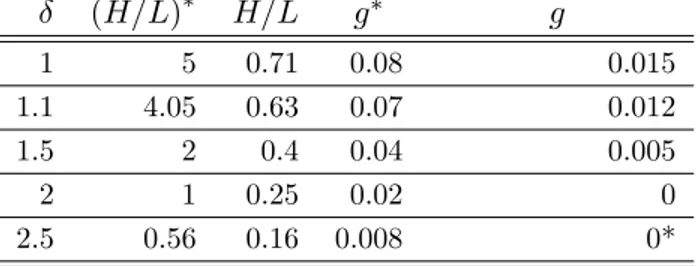
Table 3 - Comparison between the DE and the SP
δ (H/L)∗ H/L g∗ g 1 5 0.71 0.08 0.015 1.1 4.05 0.63 0.07 0.012 1.5 2 0.4 0.04 0.005 2 1 0.25 0.02 0 2.5 0.56 0.16 0.008 0*
* indicates a corner solution.
Results in the table highlight the fact that the introduction of human capital composition analysis may increase the distortion between growth rates because the levels of high-tech, tech and consequently high to low-tech ratio are also distorted. The observed values of H/L (the average value for H/L in the data is 0.17) implies an entry cost of near 2. However, the pre-dicted decentralized growth rate of the economy is far from the observed10.
Some modifications to the benchmark calibration help to solve this prob-lem. Modifications in the calibration of P/aHg or the industrial share are
shown in appendix (Tables 1.B and 2.B). We continue to face a predicted high value for the entry cost in high-tech human capital.
10According to Maddison (1995), per capita GDP had increased 1.2% between 1820 and
3
Some Evidence
In this section we show some empirical results which we compare with the theoretical results. First, we concentrate on the relationship between the measures of composition of human capital and growth (g) and then, on the relationship between the same measures and development (Y ). As the benchmark measure of human capital composition we take from the last section the ratio of high-tech human capital to total human capital (HP). There are other possible measures, such as the ratio of high-tech to low-tech human capital (HL) and also the ratio between high-tech human capital and total population, (H
N). As a measure of “scale-effects”, the model suggests
total High-tech human capital.11 In the text we present results for the first
measure and we compare them with the results from other composition and level measures, which we show in appendix.
We define high-tech human capital as the enrollments in engineering, mathematics and computer science fields and low-tech human capital as the enrollment in all other fields of science.12 So, we will concentrate on the
distribution of human capital at the tertiary education level (colleges and universities). According to our model, h = HP (given P), eh = HL (given L),
H
N (given N) or even total H have a positive relationship with the growth
rate of GDP.13
11Remember that h
1−δh=
H
L. Among the composition variables ( H P,
H L,
H
N), the last one
has a serious problem of interpretation: as we are measuring high-tech human capital in tertiary education, dividing high-tech human capital in tertiary education by total work-force may under-estimate the actual proportion, as there are, of course, some proportion of non-tertiary human capital that would be classified into high-tech if we had data to do so.
12See Definition 1 and data description in appendix. Data were supplied by
UNESCO, replying to our request and corresponds to various issues of the Un-esco Statistical Yearbook from 1970 to 1997. However, enrollments and gradu-ates by major fields of education could be downloaded from the UNESCO site at http://www.uis.unesco.org/pagesen/DBEnrolTerField.asp.
13Note that h and h
1−δh are clearly directly related. Although h and H are more directly
related to g and Y in the model, h
1−δh express better the opportunity cost of investing in
We have data for these variables from 1970 until 1997, in a total of 380 observations. In order to decrease the business-cycles and measurement er-rors effects, we have divided the sample into three decades (1970 to 1979, 1980 to 1989 and 1990 to 1997 - 124, 139 and 117 observations, respectively). From the whole sample, we have excluded the ex-communist Eastern-Europe countries. We believe these countries have had strong institutional interfer-ences in the decentralized choices of becoming high and low-tech and also in economic growth.
Table 4 shows an average of some statistics on these variables across the three decades.
Table 4 - Statistics
Mean St-Dev. Maximum Minimum C(x, eh) C(x, h) C(x,HN)
h 0.14 0.09 0.54 0.002 1 0.99 0.53
e
h 0.17 0.14 1.16 0.002 0.99 1 0.47
H
N 0.003 0.003 0.022 0.000 0.53 0.47 1
3.1 Relationship between human capital composition ratio
and growth
Our model suggests a new variable that is related to economic growth, which is a measure of composition of human capital, h. In particular we will test the following relationship:
gY ∗ 100 = C + β1X (37)
where X could be the following possible variables: H/P (= h), H/L (= eh),
H/N and H. This equation is the empirical counterpart of equation (32). For each of these variables, there correspond a constant C and a parameter
β1 in terms of the parameters in the model: C = −σ(1 − α)ρ ∗ 100 and β1 =
σ(1−α)α 2100∗P
the intercept C should be near −0.5. As it is very difficult to get values for “scale-effects” terms in this expression, as is recognized by Caballero and Jaffe (1993), we assume a value of 0.12 and say that the expected value for
β1 will be near 314, according to the same benchmark values defined in the
last section (α = 0.5, ρ = 0.02, P/aHg = 0.12, σ = 0.5).
We will test these equations econometrically and we expect to find values in this range in order to verify the theory. We will use a system equation approach with three equations, one for each decade, in which we always allow for time specific intercepts15. With the two last sub-periods of the sample, we perform IV estimations which account for endogenous problems, as h is given endogenously in the model. We will, preferably, refer to them. For comparison, we also add results which assume that entry cost is equal to 2, as suggested by Table 3. Experimental results that consider entry costs between 2 and 3 introduce little changes in the t-statistics and do not change statistical significance.
Table 5 - Human Capital Composition and Economic Growth Dependent variable: growth rate of GDP per capita
Without Entry Costs Withδ = 2
Equation 1 (H/P) SUR IV SUR IV
H/P 5.69*** 8.00*** 7.18*** 10.23*** (3.35) (3.04) (3.16) (2.96) R2 0.01, 0.08 0.06, 0.06 0.00, 0.07 0.05, 0.06 0.03 0.03 Serial Correlation 0.22, 0.15 0.19 0.22, 0.15 0.19 Number Obs. 107, 116 102, 88 107, 116 102, 88 94 94
Notes: t-statistics are presented in parentheses. They are based on white-consistent variance matrix in IV estimation. Constants are omitted in the
table.
14This (0.12) is the value for δ/β of 0.119 in Caballero and Jaffe (1993). A value of 0.18
will give a β1= 4.5 and a value of 0.07 will give a value of β1= 1.75.
15This does not change the significance of the coefficients, but allows for better fit of the
models, particularly in instrumental variables estimation. This is a common procedure in the literature (see Barro and Sala-i-Martin (1995), for instance).
Table 5 shows us a direct, significant and positive effect of H/P (h) on the economic growth rate. This does not change much when entry cost in high-tech schools is increased to 2. When compared to other measures (see Table 1.C.), it can be said that the intercepts (which are not shown) vary between -0.6 and 2.13 for the SUR equations and between -1.69 and 0.67 for the IV equations, where the most positive values are obtained in equation 3 and the most negative ones in equation 4. There are three main conclu-sions: (1) the effect of the four variables are clearly significantly positive; (2) quantitatively, the value of the estimated coefficient is above the cali-bration values (at least for the composition variables, H/P, H/L and H/N ), although for the first two equations the values are in the same range (less than 10) and (3) the intercepts are near the calibrated value -0.5, at least for equations 1 and 2 in the instrumental estimation. Nevertheless, estimators of coefficients of H and HN are always far from that on calibration. These quantitative departures from the calibration procedure may indicate either a measurement error in the variables16 or an under-calibration of 1/a
Hg.
It may suggest that the productivity of the research sector is much greater than we are supposing in calibration. To reach a value of β1 = 7, we would need a value of 0.28 instead of 0.12 for the “scale-effect” term.
3.1.1 A complete specification
As a robustness test, we will introduce some control variables that may be linked with the definitions of the constants ρ and L, P and N17. For ρ, we
introduce as proxies the saving rate and life expectation. These are natural
16Which could be caused only by the way we measure high-tech human capital, because
it is the possible proxy, but may differ for the actual stock of high-tech human capital in the economy.
17We could not find an appropriate proxy for α. As is well recognized, finding a proxy for
elasticities of substitution or markups is very difficult. We kept α as part of the estimation procedure, even for robustness tests. L and P were defined previously.
proxies for the discount rate as the first is linked with the preferences trade-off between present and future consumption and the second goes along with higher health and better work habits and education, as Barro and Sala-i-Martin (1995) recognized, and may also be naturally linked with higher preference for the future, as the expected returns of savings may be higher where life expectancy is high. For N we introduce the log of working-age population, as labor force is known to have more measurement errors18. For
P , we introduce the sum of L and H, which corresponds to set δ = 1 and P = H + L. Results with δ = 2 are presented. Of course we had eliminated
variable P in the estimation of the equation with H. Results are shown in Table 6.
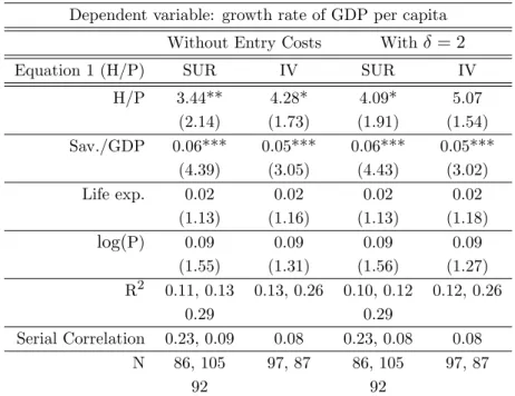
Table 6 - Robustness
Dependent variable: growth rate of GDP per capita
Without Entry Costs Withδ = 2
Equation 1 (H/P) SUR IV SUR IV
H/P 3.44** 4.28* 4.09* 5.07 (2.14) (1.73) (1.91) (1.54) Sav./GDP 0.06*** 0.05*** 0.06*** 0.05*** (4.39) (3.05) (4.43) (3.02) Life exp. 0.02 0.02 0.02 0.02 (1.13) (1.16) (1.13) (1.18) log(P) 0.09 0.09 0.09 0.09 (1.55) (1.31) (1.56) (1.27) R2 0.11, 0.13 0.13, 0.26 0.10, 0.12 0.12, 0.26 0.29 0.29 Serial Correlation 0.23, 0.09 0.08 0.23, 0.08 0.08 N 86, 105 97, 87 86, 105 97, 87 92 92
Notes: Standard-errors are presented in parentheses. They are based on white-consistent variance matrix in IV estimation. Constants are omitted in the
table.
Now, it is of course more difficult to identify parallels between estima-tion and calibraestima-tions in which (37) is concerned. However, the main result remains unchangeable. High-tech proportion seems to be positively related to economic growth conditional on proxies for the discount rate and total stocks of human capital (at tertiary education level). Here, the considera-tion of entry costs (δ = 2) decrease the significance of high-tech proporconsidera-tion, making coefficients marginally significant.
Qualitatively, the relationship between H/P, H/L and H (see Tables 6 and 2.C) and economic growth stays significantly positive, despite a full rejection of the relationship between H/N and economic growth. This may occur because this is not a good measure of composition, as we have al-ready explained. Quantitatively, the departures from calibration about β1 coefficient seem to be smaller.
We also present growth regressions using the benchmark specification in Barro (1991)19, and including h and h/(1 − h) (Table 1.D). Although far from what this model suggests as sources of growth, this is closer to the existing empirical literature and also shows a positive relationship between these variables and economic growth, following and supporting the evidence in Murphy, Shleifer and Visnhy (1991). Results in these regressions are in the spirit of Barro’s (1991) results, showing positive and significant effects of human capital (secondary enrolment), physical capital (investment) and a significant convergence effect20 and a negative effect of bad institutions
(Black Market Premium) and Government Spending, and a negative al-though weakly significant effect of Assassinations21. Although not reported
19This replicates the Barro (1991) regression, in a system equation applied to the three
decades under observation and with the use of Black Market Premium in substitution of PPP deviations of the investment deflator so as to measure market distortions and institutional differences. This is in line with more recent studies.
20A USD$1000 increase in GDP per capita would lower the economic growth rate by
0.1 to 0.2% per year.
21In the IV specification we have eliminated Assassinations because the lagged value
in Table 1.D, our data can also show a positive and significant relation-ship between the log of total high-tech human capital either in SUR or IV estimations in this Barro-regression type.
Here we can see that the positive effects of the tech and the high-low-tech ratios are consistent with the usual conditional convergence and with the positive effect of human and physical capital. The introduction of this variable does weaken the relationship between economic growth and general human capital and the negative relationship between growth and government spending, but strengthens the relationship between bad insti-tutions or market distortions (measured by Black Market Premium) and growth. These results seems to indicate that a 1% increase in growth rate of GDP per capita could occur either by a 0.35 increase in h (with a coefficient of near 3) or by a 35% increase in the secondary school enrollment (with a coefficient of 0.03)22, ceteris paribus.
3.2 Relationship between human capital composition and
development
Proof 2 and condition (34) imply that there is a non-linear relationship between Y and h. Recurring to calibration we try to determine what we should see in data. We now obtain conditions to define the sign of the total effect. We write (34) in logs and derive the expression in reference to h. This gives us the sufficient condition for a positive effect of h on GDP per
capita:
author, we have always used GDP and enrolments in the first year of the period. All the remaining differences may arise due to different periods and consequently possible different samples.
22Further research about the relationship of this measure of human capital composition
and all the growing examples of possible proxies for human capital (see Barro and Lee (1993) and Barro and Sala-i-Martin (1995)) would be interesting, but is beyond the scope of this paper.
∂ log(Yt) ∂h = σ (1 − α)2 α P aHgt + αP (σ − δh) − (1 − σ)aHgαρ (αhP + aHgαρ)(1 − δh) . (38)
The Yt that maximizes the log of (34) divides a region of total positive
effects of h on GDP from a region of total negative effects of h. Intuitively, it is possible that after some value of h, the opportunity cost of dedicating resources to produce good X or to R&D becomes so strong that the product decreases. The value of h that maximizes Ytincreases with the differentiation
of industrial products (1/α), with the share of the industrial sector (σ) and decreases with the inverse of productivity in R&D activities (aHg),
but essentially increases as time (t) passes and previous economic growth becomes more and more relevant.
Next corollary argues that we should expect an almost positive relation-ship between both variables, but a small opportunity cost of high invest-ments in high-tech could arise.
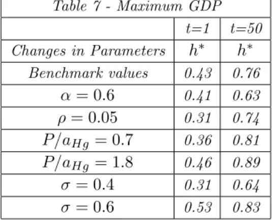
Corollary 1 We reach values for high-tech human capital ratio which
max-imize GDP per capita that suggest a positive relationship between the high-low-tech ratio and GDP per capita. The following table shows departures from the benchmark parameters in Table 2. In fact, for the more developed countries (in which, past growth rates represent much of the level of GDP per capita), countries with higher h must have higher GDP per capita.
Table 7 - Maximum GDP t=1 t=50 Changes in Parameters h∗ h∗ Benchmark values 0.43 0.76 α = 0.6 0.41 0.63 ρ = 0.05 0.31 0.74 P/aHg = 0.7 0.36 0.81 P/aHg = 1.8 0.46 0.89 σ = 0.4 0.31 0.64 σ = 0.6 0.53 0.83
We argue that values in Table 7 are hardly achieved in data (see Table 4), and so we may have an almost positive relationship between high-tech ratio and GDP per capita. There are 42 observations above h = 0.31 (the minimum value in Table 7) in data in a total of 380 (11.0%).
In conclusion, beginning with a small GDP, h increases with GDP until quite a high value of h (which increases with development) and then de-creases. It can also be said that very rich countries should always have a higher h than very poor countries and almost always higher than middle-income ones.
We will test econometrically equation (34), which we can re-state as:
log(Y ) = C + β1h + β2log(h + 0.1) + β3log(1 − h). (39) This equation is more difficult to test than the previous one. We have decided to proxy (34) by (39), where 0.1 accounts for the term aHgαρ in (34).
We have also tested (39) without this term and conclude that the results change very little. According to corollary one we would expect two clear positive effects (β1, β2 > 0) and the third effect close to zero, as we would
expect the above-mentioned opportunity cost to be quite small (β3 ≈ 0).
To avoid the expected multicollinearity problems (as these three regressors are closely related), we will only be concerned with the total positive and negative effects of h in log(Yt). First we will test the equation without the β2 term and then without the β1 term. We cannot provide IV estimations, as serial-correlations between equations are high.
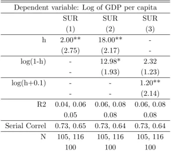
Table 8 - Human Capital Composition and Economic Development
Dependent variable: Log of GDP per capita
SUR SUR SUR
(1) (2) (3) h 2.00** 18.00** -(2.75) (2.17) -log(1-h) - 12.98* 2.32 - (1.93) (1.23) log(h+0.1) - - 1.20** - - (2.14) R2 0.04, 0.06 0.06, 0.08 0.06, 0.08 0.05 0.08 0.08 Serial Correl 0.73, 0.65 0.73, 0.64 0.73, 0.64 N 105, 116 105, 116 105, 116 100 100 100
Notes: Standard-errors are presented in parentheses. They are based on white-consistent variance matrix in IV estimation. Constants are omitted in the
table.
Results in Table 8 show that there is an overall positive relationship be-tween GDP per capita and the high-tech ratio, and that the opportunity cost also occurs with lower statistical significance, as predicted (β1, β2 > 0
although β3 > 0 also). With δ = 2 (results are not shown), the relationship
in column (1) becomes stronger but the significance of coefficients on equa-tions in columns (2) and (3) becomes weaker. However, the positive effect continue to be statistically significant in all the specifications.
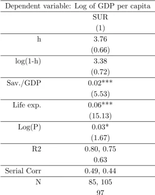
Table 9 - Robustness
Dependent variable: Log of GDP per capita SUR (1) h 3.76 (0.66) log(1-h) 3.38 (0.72) Sav./GDP 0.02*** (5.53) Life exp. 0.06*** (15.13) Log(P) 0.03* (1.67) R2 0.80, 0.75 0.63 Serial Corr 0.49, 0.44 N 85, 105 97
Notes: Standard-errors are presented in parentheses. They are based on white-consistent variance matrix in IV estimation. Constants are omitted in the
table.
Table 9 shows that all the expected results statistically fail at the usual levels under a more complete specification, although keeping the positive sign. We present only one specification (which corresponds to column (2) in Table 8), but other specifications, namely linked with that in column (3) of Table 8, would not change the results at all. We have also tested linear relationships between development and h with and without controls and polynomial relationships between GDP per capita and h. If the simple linear relationships seem to be significantly positive, the multiple regression with controls shows coefficients of h statistically not different from zero, as is the case in Table 9.
4
Conclusion
The effect of human capital composition had not been considered yet in R&D endogenous growth models. However, both historical and econometric evidence has shown some positive relationship between some types of human capital and economic growth. Furthermore, we have pointed out that the allocation of human capital (from tertiary education) differ across sectors in the economy.
We introduced these features in a simple and standard increasing-variety R&D model of endogenous growth. Thus the model accounts for human cap-ital composition, in the sense that only high-tech human capcap-ital participate in R&D activities and predicts a positive relationship between growth and different possible measures of human capital composition (high-tech human capital ratio, for instance). It also predicts an almost always positive re-lationship between the ratio and the level of GDP. Moreover, it introduces an endogenous choice between different types of human capital. A crucial variable is the entry cost in high-tech schools. When this cost increases it lowers the stock of the human capital employed in R&D labs and then decreases economic growth. These highlights potentially interesting policy implications of this entry cost, as it has direct influence on human capital composition and indirect influence on economic growth. This variable may be influenced through education policy.
This model also shows that the social planner GDP growth rate is above that of decentralized equilibrium, and that spillovers and monopolies also introduce a distortion in the optimal decision of investing in high-tech and low-tech human capital. Specifically, our model suggests that there is a lower high to low-tech human capital ratio in the decentralized equilibrium than in the social planner solution. Additionally, this consideration of human capital composition also quantitatively increases the traditional distortion in the growth rate of GDP per capita.
The use of an ideas-based growth model (Grossman and Helpman (1991) type) with constant returns to scale in the production of ideas deserves some discussion, as this is a crucial assumption to have a theoretical relationship between growth rates and the level and the proportion of high-techs, which is indeed verified in data. This kind of model implies the so-called “scale-effect”, which supports that: (1) the economy growth rate is directly related with its dimension and (2) as a consequence, the growth rate of the economy becomes explosive when its dimension (e.g. population) increases. The data evidence of increasing population with no explosive economic growth is the most striking evidence for rejection of these models, although cross-section studies do not show clear evidence of rejection of a positive relationship between growth rates and population (see Barro and Sala-i-Martin (1995) and our own results). The existence of the scale-effect has been rejected with time-series tests, however (Jones (1995b)). This has led Jones (1995a) to propose a new model where the economy’s growth rate is directly related with population growth. However, as the author recognizes, “the model still contains a very strong prediction for scale effects” (Jones, 1995a), as an economy with more researchers will grow faster in the transition to the steady-state, which goes along with the evidence of Kremer (1993) on a cross-sectional or long-run “scale-effect”.
We believe this is a plausible model to explain the evidence on human capital composition because it predicts a steady-state ratio of high to low tech human capital (which in a model like that of Jones (1995a) would not be possible) which enables a clearer perception of the determinants of the composition of human capital (high and low-tech) and its influence on growth and development, which are the main objectives of this research.
Finally, we test the theoretical implications of the model using data from human capital composition in tertiary education level, as data on entry-costs are unavailable. We also deal with possible endogeneity of human capital
composition variables, as suggested by the model. Proposed measures of hu-man capital composition are positively related to growth and, less robustly, to the level of development, measured as GDP per capita. In fact, esti-mations also show a small direct opportunity cost of investing in high-tech human capital.
Some motivation to future research is linked with the exploration of the relationship of human capital composition variables with other traditional variables of human capital and with the explanation of different levels of the proposed measures of human capital composition across countries. With-out a clear positive relationship between high-tech proportion and GDP per
capita (as Jones (1995b) predicted for human capital employed in R&D23), exploring the data relationship between these variables and the level of de-velopment becomes an interesting path to follow. It could also be interesting to extend this model to a setting of increasing quality, as this setup allows for over-investment in R&D where our model increases the tendency to under-invest in R&D.
References
[1] Acemuglu (2001), Good jobs versus bad jobs, Journal of Labor Eco-nomics, 19(1), January, 1-21.
[2] Bertocchi, G. and Spagat, M. (1998), The evolution of modern
educa-tional systems: technical versus general education, distribueduca-tional
con-flict and growth, CEPR Discussion paper 1925.
[3] Barro, R. (1991), “Economic growth in a cross section of countries”,
Quarterly Journal of Economics, May, vol. CVI, number 2, pp.
407-444.
[4] Barro, R. and Sala-i-Martin, X. (1995), Economic Growth, McGraw-Hill.
[5] Barro, R. (1999), Human Capital and Growth in Cross Country Re-gression, Swedish Economic Policy Review, number 6.
[6] Becker, G., Murphy, K. and Tamura, R. (1990), “Human capital, fertil-ity, and economic growth”, Journal of Political Economy, vol. XCVIII, pp.12-37.
[7] Caballero, R. and Jaffe, A. (1993), “How high are the giants’ shoulders: an empirical assessment of knowledge spillovers and creative destruction in a model of economic growth”, NBER Macroeconomics Annual. [8] Crafts, N.F.R. (1995), “Exogenous or endogenous growth? The
Indus-trial Revolution reconsidered”, The Journal of Economic History, Vol. 55, number 4, December
[9] Funke, M. and H. Strulik (2000), On Endogenous growth with phys-ical capital, human capital and product variety, European Economic
Review, 44, pp.491-515.
[10] Grossman, G. and Helpman, E. (1991), Innovation and Growth in the
global economy, MIT press.
[11] Iyigun, M. and Owen, A. (1999), “Entrepreneurs, Professionals and Growth”, Journal of Economic Growth, vol. 4, number 2, pp. 215-232. [12] Jones, C. (1995a), R&D-based models of endogenous growth, Journal
of political Economy, vol. 103, n.4.
[13] Jones, C. (1995b), Time-series tests of endogenous growth models, Quarterly Journal of Economics, 100, pp.495-525.
[14] Lucas, R. (1988), “On the Mechanics of Development Planning”,
[15] Maddison, A. (1995), Monitoring the World Economy 1820-1992, De-velopment Center Studies, OECD, Paris
[16] Maddison, A. (2001), The World Economy, a millenial perspective, De-velopment Center Studies, OECD, Paris
[17] Murphy, K., Shleifer, A. and Vishny, R. (1991), “The Allocation of talent: implications for growth”, Quarterly Journal of Economics, May, volume CVI, 2, pp. 503-530.
[18] Nelson, R. and Phelps, E. (1966), “Investment in Humans, Techno-logical diffusion and Economic Growth”, American Economic Review
Proceedings, vol. LVI, pp.69-75.
[19] Romer, P. (1990), “Endogenous Technological change”, Journal of
Po-litical Economy, vol. XCVIII, pp.71-102.
[20] Temple, J. and Voth, H.(1998), “Human capital, equipment investment, and industrialization”, European Economic Review, 42, pp. 1343-1362.
A
Proofs of Propositions
Proof. (PROPOSITION 1) Part (1). Solving simultaneously (25) and (28) gives us the varieties growth rate, which is given in function of the stocks of high-tech and low-tech workers:
g = (1 − β)H +
1
ωL aHg
− βρ, where β = (1 − σ(1 − α)) (40) Dividing (21) by (22), we reach a steady-state H/L ratio, which depends on the relative wage.
H L = 1 ω g ρ+g(1 − α)σ + σα 1 − σ (41)
Solving (40) and (41) simultaneously gives us the steady-state high-tech to low-tech human capital ratio. First we have constructed the term ρ+gg (1−
α)σ beginning with (40). Then we solved a quadratic equation on HL and eliminated the negative root24. The positive root of the equation is then:
H L = 1 ω σ 1 − σ − ρaHg L (42) In order to get a H
L ratio independent of L, we set ω = δ to get an entry
cost of high-tech which is not time-dependent and re-defined the variables, setting L + δH = P so as to have h = H
P and 1 − δh = PL, where P is the
total labor force in the model (the sum of high-tech and low-tech human capital). Making the necessary substitutions, we get our result of high-low tech ratio in (29).
Part (2). Using the re-definition of variables made in part (1) and (29), we can simplify the growth rate of varieties (40) to:
24The quadratic equation was ωL a( H L) 2+ (1−2σ 1−σ L a + ρω) H L + (ρ − σ ω(1−σ) L a) = 0.
g = (1 − β)( h 1 − δh+ 1 δ) P aHg(1 − δh) − βρ where β = 1 − (1 − α)σ (43)
Using 1δ given by (29) we get to our second result (30). Also with h that is given by h = 1 δ £ σ − δ(1 − σ)ρaHg P ¤
, which is directly calculated from (29), we easily reach equation (31).
Proof. (PROPOSITION 2) First we use (10) to substitute D for X in GDP function (5). Then we replace X and Z from (19) and (20), respectively, in (5). We obtain: Yt= nσ1−αα (aLZ aHx )σ( h 1 − δh− aHgg 1 − δh 1 P) σ(1 − δh) P aLZ (44) Next we set nt = n0egt, where n
0 is an initial value of the number of
varieties, and finally we substitute (30) in (44) to get the expression in the proposition.
Proof. (THEOREM 1) The current value Hamiltonian is the following:
£ = log à nσ1−αα µ Hx aHx ¶σµ P − δH aLz ¶1−σ! + λ(H − Hx agH ) (45)
From this we get the first order conditions:
(H) − (1 − σ)δ P − δH + λ a = 0 (46) (Hx) Hσ x − λ a = 0 (47) (N ) σ1 − α α = ρλ − · λ (48)
Dividing the first FOC by the second and using P − δH = L, we get L Hx =
δσ
1−σ. In addition, from the third FOC, we achieve the following growth rate
for the multiplier:
· λ λ = ρ-σ1−αα 1λ. In steady-state · λ λ = 0, because human
capital and population are constant in the model: λ = σ1 − α α 1 ρ ⇒ Hx a = ρ α 1 − α (49)
Using HLx = 1−σδσ and this last result, we get:
L = ρ α
1 − α 1 − σ
σ a (50)
As H=P −L
δ , H can be written as:
H = P − 1 δ1−αα 1−σσ ρa δ (51) Dividing H by L we get: µ H L ¶∗ = P − ρ α 1−α1−σσ a δ ³ ρ α 1−α1−σσ a ´ = 1 δ · P ρa σ 1 − σ 1 − α α 1 δ − 1 ¸ = = σ 1−σ1−αα 1δ−ρaP δρaP (52)
Then we reach (35) in the theorem. The condition under which (H/L)∗ in (35) is higher than (H/L) in (29) is the following:
P δρaHg > α 1 − α 1 σ − 1. (53)
This condition is verified for all interior solutions of the decentralized equi-librium and the social planner solution. To see this, we must note that, to have a positive growth rate of GDP per capita in the decentralized solution, for instance, we must verify a condition which implies an higher δρaPHg than that required by the latter one:
P δρaHg > α 1 − α 1 σ + σ 1 − σ 1 ρ. (54)
The same applies to a positive growth rate of the optimal solution: δρaP
Hg >
α
B
Comparing DE and SP
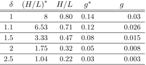
Table 1.B - DE and SP withP/aHg = 1.8
δ (H/L)∗ H/L g∗ g 1 8 0.80 0.14 0.03 1.1 6.53 0.71 0.12 0.026 1.5 3.33 0.47 0.08 0.015 2 1.75 0.32 0.05 0.008 2.5 1.04 0.22 0.03 0.003
Table 2.B - DE and SP withσ = 0.6 δ (H/L)∗ H/L g∗ g 1 8 1.14 0.09 0.02 1.1 6.53 1.01 0.08 0.018 1.5 3.33 0.67 0.05 0.01 2 1.75 0.44 0.03 0.004 2.5 1.04 0.31 0.001 0.0004
C
Alternative Measures (Low tech ratio,
High-tech total workforce ratio and high-High-tech stock)
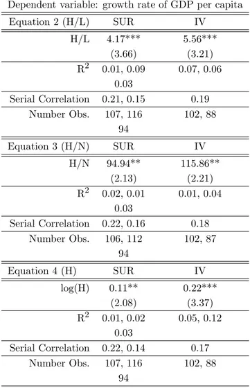
Table 1.C - Human Capital Composition and Economic Growth
Dependent variable: growth rate of GDP per capita
Equation 2 (H/L) SUR IV H/L 4.17*** 5.56*** (3.66) (3.21) R2 0.01, 0.09 0.07, 0.06 0.03 Serial Correlation 0.21, 0.15 0.19 Number Obs. 107, 116 102, 88 94 Equation 3 (H/N) SUR IV H/N 94.94** 115.86** (2.13) (2.21) R2 0.02, 0.01 0.01, 0.04 0.03 Serial Correlation 0.22, 0.16 0.18 Number Obs. 106, 112 102, 87 94 Equation 4 (H) SUR IV log(H) 0.11** 0.22*** (2.08) (3.37) R2 0.01, 0.02 0.05, 0.12 0.03 Serial Correlation 0.22, 0.14 0.17 Number Obs. 107, 116 102, 88 94
Table 2.C - Robustness
Dependent variable: growth rate of GDP per capita
Equation 2 (H/L) SUR IV H/L 2.68** 3.95** (2.50) (2.51) Sav./GDP 0.05*** 0.06*** (4.30) (3.48) Life exp. 0.02 0.01 (1.17) (0.97) log(L) 0.09 0.11 (1.55) (1.59) R2 0.12, 0.13 0.15, 0.27 0.29 Serial Correlation 0.22, 0.08 0.09 N 87, 105 98, 88 92
Table 2.C - Robustness (continued) Equation 3 (H/N) SUR IV H/N -12.11 -88.52 (-0.27) (-1.21) Sav./GDP 0.05*** 0.05*** (4.28) (2.70) Life exp. 0.04** 0.06*** (2.43) (3.16) log(N) 0.18** 0.25*** (2.63) (2.91) R2 0.08, 0.15 0.18, 0.26 0.26 Serial Correlation 0.22, 0.07 0.09 N 86, 105 97, 86 92 Equation 4 (H) SUR IV log(H) 0.11** 0.13* (1.98) (1.77) Sav./GDP 0.06*** 0.05*** (4.38) (2.92) Life exp. 0.02 0.02 (1.46) (1.29) R2 0.08, 0.12 0.12, 0.25 0.28 Serial Correlation 0.23, 0.08 0.08 N 86, 105 97, 87 92
Notes: Standard-errors are presented in parentheses. They are based on white-consistent variance matrix in IV estimation. Constants are omitted in the
D
Barro Regressions
Table 1.D. - Robustness in a Barro Growth Regression Dependent variable: growth rate of GDP per capita
SUR SUR SUR IV IV IV
(1) (2) (3) (4) (5) (6) GDP -0.0001** -0.0001* -0.0001* -0.0002*** -0.0001*** -0.0001*** (-2.48) (-1.87) (-1.90) (-3.32) (-2.28) (-3.23) Prim. Enrolment -0.0124 -0.0126* -0.0122* -0.0094 -0.0161** -0.0163** (-1.50) (-1.98) (-1.97) (-1.25) (-2.13) (-2.19) Sec. Enrolment 0.0188** 0.0135* 0.0136* 0.0330*** 0.0259** 0.0259** (2.42) (1.76) (1.76) (3.30) (2.28) (2.31) Revolutions -0.0076 0.0536 0.0407 0.4597 0.8228 0.8007 (-0.02) (0.15) (0.11) (0.68) (1.21) (1.17) Assassinations -2.0694** -1.4861 -1.4825 – – – (-2.15) (-1.06) (-1.06) – – – GCons. -0.0427*** -0.0357*** -0.0354*** -0.0454*** -0.0360** -0.0355** (-3.33) (-2.82) (-2.80) (-2.65) (-2.10) (-2.08) Inv/GDP 0.1027*** 0.1046*** 0.1053*** 0.0805*** 0.0827*** 0.0830*** (5.85) (6.02) (6.06) (2.85) (3.45) (3.44) log(1+BMP) -3.1287*** -3.4901*** -3.5004*** -3.2757*** -5.1016*** -5.1065*** (-3.67) (-4.17) (-4.17) (-2.01) (-3.28) (-3.26) h/(1-h) - 3.6898** - - 2.7289* -- (2.29) - - (1.64) -h - - 3.6638** - - 3.5323 - - (2.19) - - (1.45) R2 0.22, 0.38 0.21, 0.38 0.21, 0.38 0.38, 0.17 0.40, 0.17 0.40, 0.14 0.25 0.25 0.25 Serial Correlation 0.05, 0.11 0.02, 0.08 0.02, 0.09 0.17 0.15 0.15 N 75, 86 74, 85 74, 85 80, 84 74, 72 74, 72 94 83 83
Notes: Standard-errors are presented in parentheses. They are based on white-consistent variance matrix in IV estimation. Constants are omitted in the
E
Country List (in Table 5)
Countries in Table 5
1970-79 1980-89 1990-97 Algeria Algeria Algeria Angola Angola Angola Argentina Argentina Argentina Australia Australia Australia Austria Austria Austria Bangladesh Bahrain Bahrain Belgium Bangladesh Belgium Benin Barbados Benin Bermuda Belgium Bolivia
Bolivia Benin Botswana Botswana Bhutan Brazil
Brazil Bolivia Burkina Faso Burkina Faso Botswana Burundi
Burundi Brazil Cameroon Cameroon Burkina Faso Canada
Canada Burundi Central African Republic Central African Republic Cameroon Chad
Chad Canada Chile
Chile Central African Republic China China Chile Colombia Colombia China Congo, Rep.
drc Colombia Costa Rica Congo Democratic Rep. of the Congo Cote d’Ivoire Costa Rica Congo Denmark
Cyprus Costa Rica Dominica Denmark Ivory Coast Dominican Republic Dominican Republic Cyprus Ecuador
Ecuador Denmark Egypt, Arab Rep. Egypt Dominican Republic El Salvador El Salvador Ecuador Equatorial Guinea
Ethiopia Egypt Ethiopia Finland El Salvador Finland France Ethiopia France
Gabon Fiji Ghana
Ghana Finland Greece Greece France Guinea Guinea Gabon Honduras
Countries in Table 5 (cont.)
1970-79 1980-89 1990-97 Guyana Greece Iceland Haiti Grenada India Honduras Guinea Indonesia China, Hong Kong SAR Guyana Ireland
Iceland Haiti Israel Indonesia Honduras Italy Iran, Islamic Republic of China, Hong Kong SAR Jamaica
Iraq Iceland Japan Ireland India Jordan Israel Indonesia Kenya Italy Iran, Islamic Republic of Korea, Rep. Jamaica Ireland Lesotho
Japan Israel Madagascar Jordan Italy Malawi
Kenya Jamaica Malaysia Korea, Republic of Japan Malta
Kuwait Jordan Mauritania Lesotho Kenya Mauritius
Liberia Mexico
Luxembourg Kuwait Mongolia Madagascar Lesotho Morocco Malawi Luxembourg Mozambique Malaysia Madagascar Nepal
Mali Malawi Netherlands Malta Malaysia Nicaragua Mauritius Mali Nigeria
Mexico Malta Norway Morocco mauritania Pakistan Mozambique Mauritius Panama
Myanmar Mexico Papua New Guinea Nepal Morocco Paraguay Netherlands Mozambique Peru New Zealand Nepal Philippines
Nicaragua Netherlands Portugal Niger New Zealand Saudi Arabia Nigeria Nicaragua Senegal Norway Niger South Africa Pakistan Nigeria Spain