WORKING PAPER SERIES
CEEAplA WP No. 11/2011
The Predictive Power of Structural Models of
Corporate Debt Pricing
João C. A. Teixeira
The Predictive Power of Structural Models of Corporate
Debt Pricing
João C. A. Teixeira
Universidade dos Açores (DEG)
e CEEAplA
Working Paper n.º 11/2011
Abril de 2011
CEEAplA Working Paper n.º 11/2011 Abril de 2011
RESUMO/ABSTRACT
The Predictive Power of Structural Models of Corporate Debt Pricing
This paper tests empirically the performance of three structural models of corporate bond pricing: those of Merton (1974), Leland (1994) and Fan and Sundaresan (2000). We show that both Merton and Leland models overestimate bond prices while Fan and Sundaresan reveals an extremely good performance. When considering the prediction of credit spreads, the three models underestimate market spreads but, again, Fan and Sundaresan has a better performance. We find a rating, maturity, asset volatility and sector effect in the prediction power, as the models underestimate less the spreads of riskier firms and of bonds with better rating quality and longer maturity. Moreover, we find that spread errors are systematically related with some bond and firm’s specific variables, as well as term structure variables. Finally, an econometric model developed for equityholders bargaining power shows that it depends on proportional liquidation costs, firm’s size and distance to default.
Keywords: structural models, corporate debt valuation, empirical credit
spreads
JEL classification: G12, G13
João C. A. Teixeira Universidade dos Açores
Departamento de Economia e Gestão Rua da Mãe de Deus, 58
The predictive power of structural models of
corporate debt pricing
João C. A. Teixeira
University of the Azores - Department of Economics and Business CEEAplA
Rua Mãe de Deus, s/n 9501-801 Ponta Delgada, Portugal
Abstract
This paper tests empirically the performance of three structural models of corporate bond pricing: those of Merton (1974), Leland (1994) and Fan and Sundaresan (2000). We show that both Merton and Leland models overestimate bond prices while Fan and Sundaresan reveals an extremely good performance. When considering the prediction of credit spreads, the three models underestimate market spreads but, again, Fan and Sundaresan has a better performance. We find a rating, maturity, asset volatility and sector effect in the prediction power, as the models underestimate less the spreads of riskier firms and of bonds with better rating quality and longer maturity. Moreover, we find that spread errors are systematically related with some bond and firm’s specific variables, as well as term structure variables. Finally, an econometric model developed for equityholders bargaining power shows that it depends on proportional liquidation costs, firm’s size and distance to default.
Keywords: structural models, corporate debt valuation, empirical credit spreads
1. Introduction
The aim of this paper is to test empirically the performance of three structural models of corporate debt pricing, namely Merton (1974), Leland (1994) and Fan and Sundaresan (2000). With the analysis of prediction errors we evaluate how well can these models fit bond prices and credit spreads. We believe this is important because this allows for a discussion of which “real world features” are not captured by these models. On the other hand, a comparison of the results of the three models permits to determine the extent to which some innovations in the models have improved the pricing of risky bonds. We refer specifically to the possibility of early default, coupons, taxes and bankruptcy costs when we compare Merton (1974) model with Leland (1994) and the effect of strategic debt service when we compare Leland (1994) model with Fan and Sundaresan (2000).
Moreover, we evaluate whether there are differences in the performance of the models according to rating and maturity of the bonds or according to asset volatility and sector of the firms. This analysis seems important because the previous empirical studies in the field are not much conclusive. While Ericsson and Reneby (2002) report a better performance of Merton model for speculative grade bonds, Eom et al (2004) do not confirm that pattern in their sample.
Even considering important the analysis of a rating, maturity and asset volatility effect, the study of a sector effect is probably more important as there is very little empirical evidence regarding this issue. We believe that the study of a sector effect in the performance of the structural models is indeed one of the main contributions of this dissertation. If we detect any sector effect, then it would be interesting to analyze which characteristics of these sectors can try to explain a better or worst performance.
Another important issue that deserves our attention is the study of systematic prediction errors. Are there any bond specific, firms specific or market variables that play a systematic relationship with spread errors? Among other factors, we intend to study the influence of size, leverage, maturity, rating, asset volatility and firm growing opportunities in the performance of the models. This is important not only because the existing empirical literature sometimes found some contradictory results in this analysis but also because we introduce some new explanatory variables, as the yield to maturity and the market-to-book ratio (as a proxy for growing opportunities).
As far as we are concerned, this paper is the first study that calibrates and evaluates the performance of Fan and Sundaresan (2000) model. There are some calibrations of strategic debt services models as the one by Mella-Barral and Perraudin (1997) in Huang and Huang (2002) paper. However, they do not explicitly calibrate Fan and Sundaresan (2000) model. Furthermore, we introduce an econometric model that tries to explain equityholders bargaining power at liquidation.
To implement the empirical study properly, we structure this paper as follows. First, we explain the process of data gathering and the calibration procedure adopted to implement the models. Then follows the empirical results section where we discuss the performance of the models and the systematic prediction errors. Finally, there is the conclusion where we summarize the main findings of the dissertation.
2. Empirical Implementation
This section is organized in two parts. First we describe the process of data gathering and secondly we present the calibration procedure used to estimate the parameters of the models. We provide a specific description of the estimation of each model’s parameters. The implementation of the numerical methods is conducted in Excel using Solver.
2.1 Data
In order to test empirically the models presented earlier it is important to select a sample of companies with simple capital structures. Ideally we should have companies with zero coupon bonds when testing the Merton (1974) model and companies with perpetual bonds when testing the Leland (1994) and the Fan and Sundaresan (2000) models. However, since it is not always possible to find these “perfect” bonds in the markets, the most reasonable approach consists in selecting bonds that have reliable prices and straightforward cashflows. An attempt to use these models to price corporate debt of firms with complex capital structures would raise doubts as to whether pricing errors are due to the assumptions of the models or to their inability to price this sort of debt. This approach has also been adopted in previous empirical studies like the one by Eom et al (2004), Ericson and Reneby (2002) and Lyden and Saraniti (2000). While the first two studies use companies with simple capital structures but with more than one traded bond, Lyden and Saraniti (2000) limit the sample to companies with only one bond.
The first selection criteria used in this study consists in limiting the sample to U.S. non-financial firms with no more than three bonds (issued in U.S. dollars). As noticed by Eom et al (2004) the leverage ratio of financial firms are not comparable to other firms. “Financial firms, such as banks, routinely have leverage ratios above 90%, whereas only the least creditworthy non-financial firms use as much debt” (p.4). In addition, the following criteria are applied:
• Consider only coupon bonds with all principal retired at maturity (bullet bonds). • Do not include bonds with option features like callable, convertible or putable
bonds.
• Do not include floating-rate bonds or bonds with sinking fund provisions.
• Do not include bonds with time to maturity less than one year, as they are unlikely to trade (suggested by Eom et al, 2004).
Following these criteria and using DATASTREAM information an initial sample of 39 companies was obtained. In order to assure the straight application of these criteria, there was a double check of the characteristic of the bonds by consulting their prospectus on EDGAR database1. After that, two companies had to be eliminated since their bonds had call features. Furthermore, in order to assure some reliability of the bond prices, all the bonds with the same quote for more than two months (despite the changes in interest rates) were excluded. With this refinement the sample was reduced to 30 companies.
As final criterion to select the sample there is the requirement that all these companies have publicly traded stock. Stock prices are not only required to compute the market value of equity but also to compute the stock volatility. An inspection in stock prices obtained from DATASTREAM allowed to detect one company that was considered an outlier, which was consequently eliminated from the sample. This company entered in bankruptcy in 2003 and its stock price was around zero in the first quarter of 2004. In the end there were left 29 companies with a total of 50 bonds.
As regards the time-period of the study, it was set as the period between October 2001 and the end of March 2004. Since DATASTREAM does not provide bond price information prior to 28/09/2001 it was not possible to extend this period.
Another important issue of the data selection process is the frequency of the data. As some of the variables of the study rely on accounting data we have to make bond information “compatible” with accounting information. This being so, and trying to maximize the number of observations in the time series, it was decided to use quarterly observations. In total there are 11 quarters of data for 27 companies and 10 quarters for 2 companies2, creating 317 observations on which the pricing performance and model specification is carried out. This sample can be compared to the one used by Jones et al (1984) which consists of a total of 27 firms, Ericsson and Reneby (2002) with 171 firms and that of Eom et al (2004) with 182 companies.
1 EDGAR database is available at SEC (U.S. Securities and Exchange Commission) web site www.sec.gov.
2
The first company with only 10 quarters of data is United Technologies because the two bonds of this company were issued after 30/10/2001, missing the first quarter of data. The second company is
Company Bond Face Value
($M) Issue Date Maturity Date Coupon
S&P Rating Yield Spread (bp) Industrial Bond 1 100 28/06/1995 01/07/2005 6.700% A 149.7 Bond 2 250 07/08/2001 15/08/2008 6.500% A 114.5 CNF Inc Bond 1 200 03/03/2000 01/05/2010 8.875% BBB- 374.1
IDEX Corp Bond 1 150 18/02/1998 15/02/2008 6.875% BBB 293.3
Pentair Inc Bond 1 250 30/09/1999 15/10/2009 7.850% BBB 247.5
Bond 1 200 14/08/2001 15/08/2011 6.250% A 107.7 Bond 2 100 28/09/1995 01/10/2005 6.625% A 119.0 Bond 1 300 24/02/1999 01/03/2009 6.750% BBB 238.5 Bond 2 100 04/09/1992 15/09/2004 7.250% BBB 301.0 Bond 1 500 24/04/2002 15/05/2012 6.100% A 75.7 Bond 2 400 23/10/2001 01/11/2006 4.875% A 73.1 Bond 1 150 19/04/2000 15/04/2010 8.500% BBB+ 283.2 Bond 2 100 29/04/1999 01/05/2009 6.500% BBB+ 236.7 Bond 1 250 07/04/1999 01/04/2009 6.000% A+ 132.6 Bond 2 240 02/02/2001 01/02/2006 6.400% A+ 121.6 Average 219.3 6.803% 191.2 Consumer Cyclical
Choice Hotels Int. Inc Bond 1 100 19/10/1998 01/05/2008 7.125% BBB- 339.7
Knight Ridder Inc Bond 1 300 23/03/1999 15/03/2029 6.875% A 148.1
Bond 1 125 21/05/1998 01/06/2028 7.125% BBB 223.5 Bond 2 125 21/05/1998 01/06/2008 6.650% BBB 195.8 Bond 1 300 11/03/1998 15/03/2028 6.950% A- 200.9 Bond 2 250 14/01/1999 15/01/2009 5.625% A- 175.5 Bond 1 200 07/08/1997 15/08/2007 7.125% BBB- 224.2 Bond 2 325 25/09/2002 01/10/2012 7.375% BBB- 129.2 Bond 3 325 26/02/2003 01/10/2012 7.375% BBB- 102.2
Unifi Inc Bond 1 250 05/02/1998 01/02/2008 6.500% B+ 763.8
Average 230.0 6.873% 250.3
Nordstrom Inc Neiman Marcus Group
Staples Inc Vulcan Materials Bemis Co Inc
Temple Inland Inc United Techonologies USF Corp
Snap-on Inc
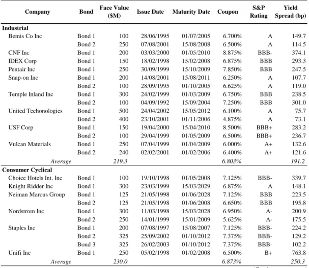
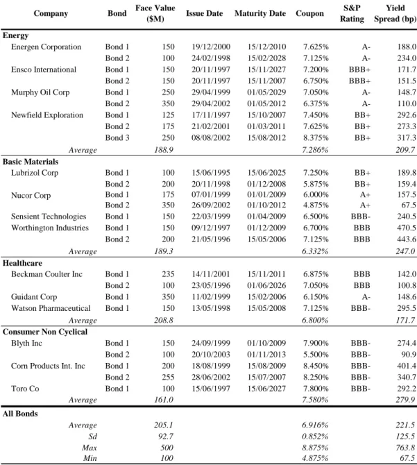
The firms are grouped in a total of six sectors, namely Industrial (9 firms), Consumer Cyclical (6 firms), Energy (4 firms), Basic Materials (4 firms), Healthcare (3 firms) and Consumer Non-Cyclical (3 firms). This grouping is based on Thomson ONE Banker sector convention (Source: http://banker.analytics.thomsonib.com/ta/).
Table 2.1 presents summary statistics on the 50 bonds in the sample. There are a total of 10 companies with just one traded bond, 17 companies with two traded bonds and only 2 companies with three traded bonds. The average coupon rate for all bonds is 6.916%, ranging from 4.875 to 8.875%. The Consumer Non-Cyclical sector has the bonds with highest coupons and, not surprisingly, is also the one with the highest average yield spread, namely 279.9 basis points. The average yield spread is 221.5 basis points for all bonds and most of the bonds (88% of the sample) are investment grade bonds (rated BBB- or higher). A more detailed analysis of rating and distribution of credit spread is conducted in section 5.1.
Table 2.1 – Bonds Summary Statistics
Company Bond Face Value
($M) Issue Date Maturity Date Coupon
S&P Rating Yield Spread (bp) Energy Bond 1 150 19/12/2000 15/12/2010 7.625% A- 188.0 Bond 2 100 24/02/1998 15/02/2028 7.125% A- 234.0 Bond 1 150 20/11/1997 15/11/2027 7.200% BBB+ 171.7 Bond 2 150 20/11/1997 15/11/2007 6.750% BBB+ 151.5 Bond 1 250 29/04/1999 01/05/2029 7.050% A- 148.7 Bond 2 350 29/04/2002 01/05/2012 6.375% A- 110.0 Bond 1 125 17/11/1997 15/10/2007 7.450% BB+ 292.6 Bond 2 175 21/02/2001 01/03/2011 7.625% BB+ 273.3 Bond 3 250 08/08/2002 15/08/2012 8.375% BB+ 317.3 Average 188.9 7.286% 209.7 Basic Materials Bond 1 100 15/06/1995 15/06/2025 7.250% BB+ 189.8 Bond 2 200 20/11/1998 01/12/2008 5.875% BB+ 159.4 Bond 1 175 07/01/1999 01/01/2009 6.000% A+ 157.5 Bond 2 350 26/09/2002 01/10/2012 4.875% A+ 67.5
Sensient Technologies Bond 1 150 22/03/1999 01/04/2009 6.500% BBB- 240.5
Bond 1 150 09/12/1997 01/12/2009 6.700% BBB 470.5 Bond 2 200 21/05/1996 15/05/2006 7.125% BBB 443.6 Average 189.3 6.332% 247.0 Healthcare Bond 1 235 14/11/2001 15/11/2011 6.875% BBB 142.0 Bond 2 100 23/05/1996 01/06/2026 7.050% BBB 100.8
Guidant Corp Bond 1 350 11/02/1999 15/02/2006 6.150% A- 148.6
Watson Pharmaceutical Bond 1 150 13/05/1998 15/05/2008 7.125% BBB- 295.5
Average 208.8 6.800% 171.7
Consumer Non Cyclical
Bond 1 150 24/09/1999 01/10/2009 7.900% BBB- 274.4 Bond 2 100 20/10/2003 01/11/2013 5.500% BBB- 90.9 Bond 1 200 18/08/1999 15/08/2009 8.450% BBB- 401.4 Bond 2 255 28/06/2002 15/07/2007 8.250% BBB- 340.7 Toro Co Bond 1 100 15/06/1997 15/06/2027 7.800% BBB- 292.2 Average 161.0 7.580% 279.9 All Bonds Average 205.1 6.916% 221.5 Sd 92.7 0.852% 125.5 Max 500 8.875% 763.8 Min 100 4.875% 67.5 Blyth Inc
Corn Products Int. Inc Newfield Exploration
Lubrizol Corp Nucor Corp
Worthington Industries
Beckman Coulter Inc Energen Corporation Ensco International Murphy Oil Corp
Table 2.1 – Bonds Summary Statistics (Cont.)
Table 2.1 reports descriptive statistics for the bonds in the sample. All the information regarding face value, issue date, maturity date, coupon and yield spread was obtained from DATASTREAM. The yield spread for each bond is an average of the spread over US treasury bills for the sample period. Rating information was obtained from Standard & Poors (www.standardandpoors.com).
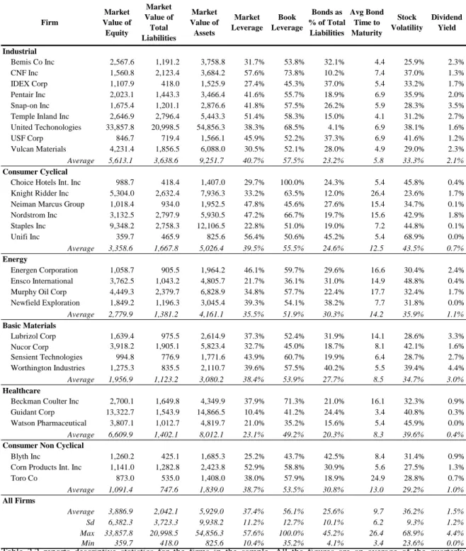
As mentioned earlier, the implementation of the model requires some accounting information, namely information about the liability structure of the firm. Quarterly balance sheets for each company were obtained from EDGAR database. Table 2.2 lists some descriptive statistics about the firms.
Firm Market Value of Equity Market Value of Total Liabilities Market Value of Assets Market Leverage Book Leverage Bonds as % of Total Liabilities Avg Bond Time to Maturity Stock Volatility Dividend Yield Industrial Bemis Co Inc 2,567.6 1,191.2 3,758.8 31.7% 53.8% 32.1% 4.4 25.9% 2.3% CNF Inc 1,560.8 2,123.4 3,684.2 57.6% 73.8% 10.2% 7.4 37.0% 1.3% IDEX Corp 1,107.9 418.0 1,525.9 27.4% 45.3% 37.0% 5.4 33.2% 1.7% Pentair Inc 2,023.1 1,443.3 3,466.4 41.6% 55.7% 18.9% 6.9 35.9% 2.0% Snap-on Inc 1,675.4 1,201.1 2,876.6 41.8% 57.5% 26.2% 5.9 28.3% 3.5% Temple Inland Inc 2,646.9 2,796.4 5,443.3 51.4% 58.3% 15.0% 4.1 31.2% 2.7% United Techonologies 33,857.8 20,998.5 54,856.3 38.3% 68.5% 4.1% 6.9 38.1% 1.6% USF Corp 846.7 719.4 1,566.1 45.9% 52.2% 37.3% 6.9 41.6% 1.2% Vulcan Materials 4,231.4 1,856.5 6,088.0 30.5% 52.1% 28.0% 4.9 29.0% 2.3% Average 5,613.1 3,638.6 9,251.7 40.7% 57.5% 23.2% 5.8 33.3% 2.1%
Consumer Cyclical
Choice Hotels Int. Inc 988.7 418.4 1,407.0 29.7% 100.0% 24.3% 5.4 45.8% 0.4% Knight Ridder Inc 5,304.0 2,632.4 7,936.3 33.2% 63.5% 12.0% 26.4 23.6% 1.7% Neiman Marcus Group 1,018.4 934.0 1,952.5 47.8% 45.6% 27.6% 15.4 34.7% 0.1% Nordstrom Inc 3,132.5 2,797.9 5,930.5 47.2% 66.7% 19.7% 15.6 42.9% 1.8% Staples Inc 9,348.2 2,758.3 12,106.5 22.8% 51.0% 19.0% 7.2 44.8% 0.1% Unifi Inc 359.7 465.9 825.6 56.4% 50.6% 45.2% 5.4 68.9% 0.0% Average 3,358.6 1,667.8 5,026.4 39.5% 55.5% 24.6% 12.5 43.5% 0.7% Energy Energen Corporation 1,058.7 905.5 1,964.2 46.1% 59.7% 29.6% 16.6 30.4% 2.4% Ensco International 3,762.5 1,043.2 4,805.7 21.7% 36.1% 31.0% 14.9 48.8% 0.4% Murphy Oil Corp 4,449.3 2,379.7 6,828.9 34.8% 57.7% 22.4% 17.7 32.4% 1.7% Newfield Exploration 1,849.2 1,196.3 3,045.4 39.3% 54.1% 38.2% 7.7 31.8% 0.0% Average 2,779.9 1,381.2 4,161.1 35.5% 51.9% 30.3% 14.2 35.9% 1.1% Basic Materials Lubrizol Corp 1,639.4 975.5 2,614.9 37.3% 52.4% 31.9% 14.1 28.6% 3.3% Nucor Corp 3,918.2 1,905.1 5,823.4 32.7% 45.0% 18.7% 8.1 42.1% 1.6% Sensient Technologies 994.8 776.9 1,771.6 43.9% 60.7% 19.9% 6.4 28.7% 2.7% Worthington Industries 1,275.3 835.5 2,110.7 39.6% 57.5% 40.2% 5.5 39.4% 4.4% Average 1,956.9 1,123.2 3,080.2 38.4% 53.9% 27.7% 8.5 34.7% 3.0% Healthcare
Beckman Coulter Inc 2,700.1 1,649.8 4,349.9 37.9% 71.3% 21.0% 16.1 32.3% 0.9% Guidant Corp 13,322.7 1,543.9 14,866.5 10.4% 41.2% 24.4% 3.4 40.8% 0.3% Watson Pharmaceutical 3,807.1 1,012.7 4,819.7 21.0% 35.2% 15.6% 5.4 45.9% 0.0% Average 6,609.9 1,402.1 8,012.1 23.1% 49.2% 20.3% 8.3 39.6% 0.4%
Consumer Non Cyclical
Blyth Inc 1,260.2 425.1 1,685.3 25.2% 43.7% 42.5% 8.4 31.4% 0.9% Corn Products Int. Inc 1,141.0 1,282.8 2,423.8 52.9% 58.8% 30.9% 5.6 27.5% 1.3% Toro Co 873.0 535.0 1,408.0 38.0% 57.9% 18.9% 24.9 28.8% 0.7% Average 1,091.4 747.6 1,839.0 38.7% 53.5% 30.8% 13.0 29.2% 1.0% All Firms Average 3,886.9 2,042.1 5,929.0 37.4% 56.1% 25.6% 9.7 36.2% 1.5% Sd 6,382.3 3,723.3 9,938.2 11.2% 12.7% 10.1% 6.2 9.3% 1.2% Max 33,857.8 20,998.5 54,856.3 57.6% 100.0% 45.2% 26.4 68.9% 4.4% Min 359.7 418.0 825.6 10.4% 35.2% 4.1% 3.4 23.6% 0.0%
Table 2.2 – Firms Summary Statistics
Table 2.2 reports descriptive statistics for the firms in the sample. All the figures are an average of the quarterly observations for each company (third quarter of 2001 until first quarter of 2004). The market value of equity and dividend yield for each quarter was obtained from DATASTREAM as well as stock prices required to compute stock volatility. Stock volatility for each quarter is the annualised stock volatility. It was computed using a series of daily log returns from the last 250 trading days preceding each quarter. Daily stock prices were also downloaded from DATASTREAM. The market value of total liabilities is the sum of the market value of traded bonds and book value of other liabilities.
The firms in the sample are reasonably large, as the average market value of assets is around $6 billion. For most companies, the market leverage (average 37.4%) is substantially below the book leverage (average 56.1%).
A more detailed analysis of the liability structure reveals that, on average, the market value of traded bonds does not represent more than 25.6% of total liabilities. These figures are very similar to previous empirical studies on structural models, namely the one by Lyden and Saraniti (2000). The sector with the highest proportion of traded bonds in total liabilities is the Consumer Non-Cyclical with 30.8%. Bond time to maturity range from 3.4 to 26.4 years but the average is around 9.7 years.
Another interesting statistic is the high stock volatility of these firms (36.2% on average). This feature is somewhat related with the high volatility period and downward in the U.S. economy that followed the September 11. Revealing its dependence on the market evolution, the Consumer Cyclical sector presents the highest volatility of the all sample (43.5%). Even though there is some dispersion among sectors, it should be noticed that the dividend yield of the sample is relatively low (1.5%). In the Healthcare sector it is no more than 0.4% but in the Basic Material sector it is near 3.0%.
3
. Empirical Results
This section is organized in four topics. First, we analyse the distribution of credit spreads and Risk Neutral Default Probabilities (RNDP) for the total sample and on a sectorial basis. Then, in section 3.2, we evaluate the performance of Merton and Leland models by interpreting average values of prediction errors in price, yield and spread. In section 3.3 there is a discussion of the systematic factors that may explain the spread errors of Merton model and finally, in section 3.4, Fan and Sundaresan debt/equity swap is discussed.
3.1 Distribution of Credit Spreads and RNDP
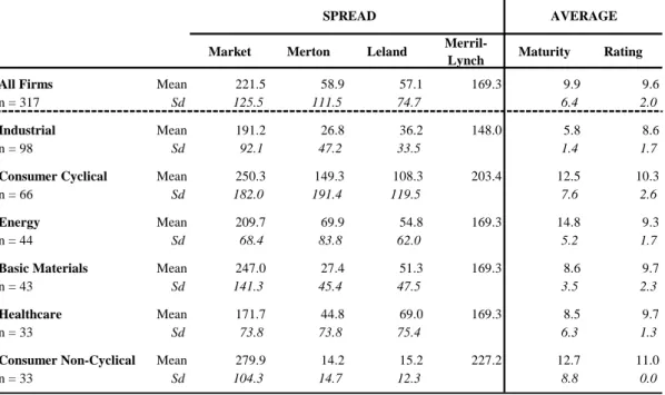
In the data section we reported information about the credit spread for each bond in the sample and averages values for each sector (presented in Table 2.1). Now, we are in position to improve this analysis, by comparing the observed credit spread with the credit spread predicted by Merton and Leland models and an approximation of credit spread based in a Merrill Lynch study, as illustrated in Table 3.1.
Table 3.1 – Descriptive Statistics of Spreads by Sectors: Market, Models and Merrill Lynch
While the market spread and the Merton and Leland predicted spreads are averages for the sample period, the Merrill Lynch spread is just an approximation of spreads considering certain intervals of years to maturity and rating of the bonds. The original study in which we based the Merrill Lynch spread presents averages spreads over the period January 1997-August 2003 for U.S. corporate bonds and was obtained from Bloomberg.
Market Merton Leland
Merril-Lynch Maturity Rating All Firms Mean 221.5 58.9 57.1 169.3 9.9 9.6
n = 317 Sd 125.5 111.5 74.7 6.4 2.0
Industrial Mean 191.2 26.8 36.2 148.0 5.8 8.6
n = 98 Sd 92.1 47.2 33.5 1.4 1.7
Consumer Cyclical Mean 250.3 149.3 108.3 203.4 12.5 10.3
n = 66 Sd 182.0 191.4 119.5 7.6 2.6
Energy Mean 209.7 69.9 54.8 169.3 14.8 9.3
n = 44 Sd 68.4 83.8 62.0 5.2 1.7
Basic Materials Mean 247.0 27.4 51.3 169.3 8.6 9.7
n = 43 Sd 141.3 45.4 47.5 3.5 2.3
Healthcare Mean 171.7 44.8 69.0 169.3 8.5 9.7
n = 33 Sd 73.8 73.8 75.4 6.3 1.3
Consumer Non-Cyclical Mean 279.9 14.2 15.2 227.2 12.7 11.0
n = 33 Sd 104.3 14.7 12.3 8.8 0.0
AVERAGE SPREAD
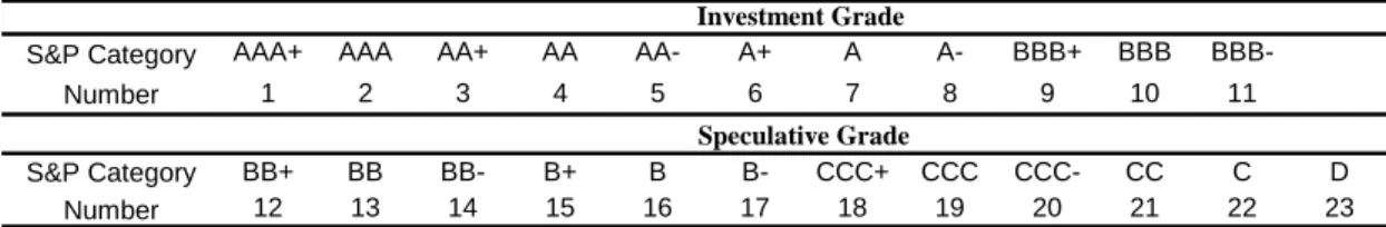
Prior to analysing these results, we should mention that, for estimation purposes, a rating conversion table was constructed. Following Eom et al (2004) and Ericsson and Reneby (2002) we assign the number one to the highest rating (AAA+) and the number 23 to the lowest rating (D). Table 5.2 reports this numerical conversion.
Table 3.2 – Rating Numerical Conversion
The first important conclusion suggested by the results of Table 3.1 is that the structural models analysed in this study underestimate the credit spread. This is true not only for the averages values of the total sample but also for the industry averages. The average market spread of the total sample is more than three times higher than the spread predicted by the Merton and Leland models (221.5 bp against 58.9 bp and 57.1 bp, respectively). The reasons why these structural models underestimate credit spreads and an industry analysis of the underestimation are discussed in more detail in the next sections.
Furthermore, Table 3.1 shows that the bonds in the sample also have an average market spread higher than the average spread presented by U.S. firms in the Merrill Lynch study (169.3 bp in this last case).
Focusing the analysis on observed credit spread, we verify that the Consumer Non-Cyclical sector has the highest spread (279.9 bp), followed by the Consumer Non-Cyclical (250.3 bp) and the Basic Materials (247.0 bp). The result of the Consumer Cyclical sector is consistent with the highest coupon rates of its bonds (already reported in Table 4.1) and also with its worst rating quality. The average rating in this sector is 11, which corresponds to BBB-, the cut-off category of investment grade bonds. In the group of bonds with the lowest market spread we have the Energy (209.7 bp), Industrial (191.2 bp) and the Healthcare (171.7 bp) sectors. These are also the sectors with the best rating, which reveals an important association between rating and market spread (the correlation between these two variables is 0.56).
S&P Category AAA+ AAA AA+ AA AA- A+ A A- BBB+ BBB
BBB-Number 1 2 3 4 5 6 7 8 9 10 11
S&P Category BB+ BB BB- B+ B B- CCC+ CCC CCC- CC C D
Number 12 13 14 15 16 17 18 19 20 21 22 23
Speculative Grade Investment Grade
0 5 10 15 20 25 30 35 40 25 50 75 100 125 150 175 200 225 250 275 300 325 035 375 400 425 450 475 050 525 550 575 600 625 650 Mor e Credit Spread (bp) Fr eque nc y
A direct comparison of the observed spreads for each sector with the spreads resulting from the Merrill Lynch study reveals that, although Merrill Lynch reports lower spreads, the ranking of sectors is quite similar. In the top spread level there is the Consumer Non-Cyclical and Consumer Cyclical sectors and in the bottom the Industrial sector (ranked fifth according to observed market spread).
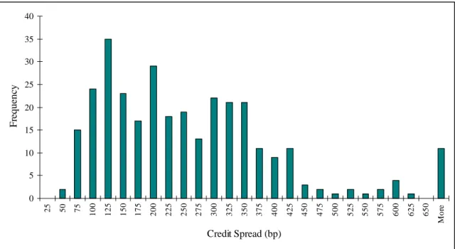
In order to improve the analysis of market spread, it is important to have an idea of its distribution. Figure 3.1 displays this distribution for the total sample.
Figure 3.1 – Distribution of Market Spread: Total Sample
The distribution of market spread is far from normal. There is a higher concentration of observations between 100 bp and 125 bp and then much more observations to the right of this range than to the left. Between 150 bp and 350 bp the frequency is quite constant and there are some important observations above 700 bp.
An industry analysis of the distribution of market spread, depicted in Figure 3.2, reveals some similarities among industries. In none of the sectors does the distribution seems to be normal and most sectors reveal a strong dispersion of credit spreads, with the exception of Energy. Panel D shows a high concentration of observations above 700 bp in the Basic Materials sector. In most sectors ranges of high frequency are followed by low frequency and again by high frequency.
0 1 2 3 4 5 6 7 25 50 75 10 0 12 5 15 0 17 5 20 0 22 5 25 0 27 5 30 0 32 5 35 0 37 5 40 0 42 5 45 0 47 5 Mo re Credit Spread (bp) Fr e q ue nc y 0 0.5 1 1.5 2 2.5 3 3.5 4 4.5 25 50 75 10 0 12 5 15 0 17 5 20 0 22 5 25 0 27 5 30 0 32 5 35 0 37 5 40 0 42 5 45 0 47 5 Mo re Credit Spread (bp) Fr e q ue n cy
Figure 3.2 – Distribution of Market Spread by Sector
Panel A – Industrial Panel B – Consumer Cyclical
Panel C – Energy Panel D – Basic Materials
Panel E – Healthcare Panel F – Consumer Non-Cyclical
In addition to the credit spread estimation reported in Table 3.1 it is important to analyse the Risk Neutral Default Probability predicted by the models, since these two variables are directly related. Table 3.3 summarises the results of this last variable. It also reports Moody’s 1-year default rates for bonds during 1999 based on cross sectional information about rating and maturity. Although this information is not directly
0 2 4 6 8 10 12 14 25 50 75 10 0 12 5 15 0 17 5 20 0 22 5 25 0 27 5 30 0 32 5 35 0 37 5 40 0 42 5 45 0 47 5 Mo re Credit Spread (bp) Fr e q ue n c y 0 1 2 3 4 5 6 7 8 9 10 25 50 75 10 0 12 5 15 0 17 5 20 0 22 5 25 0 27 5 30 0 32 5 35 0 37 5 40 0 42 5 45 0 47 5 Mo re Credit Spread (bp) Fr eq ue nc y 0 1 2 3 4 5 6 7 25 50 75 100 125 015 175 200 225 250 275 300 325 350 537 400 425 450 475 Mo re Credit Spread (bp) Fr eq ue nc y 0 2 4 6 8 10 12 14 25 50 75 100 125 150 175 200 225 250 275 300 325 350 375 400 425 450 475 Mo re Credit Spread (bp) Fr eq ue nc y
1-Year Default Rates (1999)
Merton Leland Moody's Maturity Rating All Conpanies Mean 12.3% 10.5% 0.11% 9.9 9.6
n = 317 Sd 13.7% 10.4% 6.4 2.0
Industrial Mean 7.8% 7.9% 0,00%-0,11% 5.8 8.6
n = 98 Sd 9.2% 6.1% 1.4 1.7
Consumer Cyclical Mean 22.9% 17.4% 0,11%-1,12% 12.5 10.3
n = 66 Sd 18.6% 15.0% 7.6 2.6
Energy Mean 17.1% 10.1% 0.11% 14.8 9.3
n = 44 Sd 13.2% 9.3% 5.2 1.7
Basic Materials Mean 8.1% 10.6% 0.11% 8.6 9.7
n = 43 Sd 8.4% 8.4% 3.5 2.3
Healthcare Mean 8.4% 11.8% 0.11% 8.5 9.7
n = 33 Sd 11.1% 10.2% 6.3 1.3
Consumer Non-Cyclical Mean 7.1% 3.6% 0,11%-1,12% 12.7 11.0
n = 33 Sd 7.4% 2.7% 8.8 0.0
AVERAGE RNDP
comparable with the RNDP it provides an idea of which sectors are likely to present a higher default rate.
Table 3.3 – Risk Neutral Default Probabilities (RNDP) and Moody’s 1-Year Default Rates3
As expected, the sectors with the highest predicted RNDP are also the sectors with the highest predicted spread. The Consumer Cyclical assumes the leading of this ranking with a RNDP of 22.9% predicted by the Merton model (predicted spread of 149.3 bp, Table 5.1) and 17.4% predicted by the Leland model (predicted spread of 108.3 bp). The sector with the lowest predicted RNDP (and lowest credit spread) is the Consumer Non-Cyclical, with 7.1% and 3.6% in the Merton and the Leland’s model, respectively.
There seems to be some contradiction between this ranking and the ranking based on the observed market spread. The structural models predict the lowest RNDP and the lowest credit spread for the sector with the highest market spread: Consumer Non-Cyclical. This underpricing issue will be analysed in more detail in the next section but there seems to be a reason for that particular case. The three companies of the Consumer Non-Cyclical sector reveal an historical 250 days stock volatility that is quite low, which resulted in low asset volatility estimation and consequently a high underestimation of credit spread and RNDP by the structural models.
3
Finally, taking into account cross sectional information about maturity and rating, we verify that the overall 1-year default rate is no more than 0.11%. Given its rating characteristics, the Consumer Non-Cyclical sector is the one which potentially presents a high default rate, namely between 0.11% and 1.12%. With the lowest default rate (between 0.00% and 0.11%) is the Industrial sector. This ranking in is accordance with the ranking based on the market spread and the Merrill Lynch spread of Table 3.1.
As a summary of this section we can say that the first results of the structural models reveal an underestimation of credit spreads and that both the observed credit spread and the predicted spreads are characterized by a high dispersion. The RNDP ranges from 10.5% in Leland model to 12.3% in Merton model. Even though the Consumer Non-Cyclical and the Consumer Non-Cyclical sectors have the highest market spreads, the predictions of the models are not always coincident with this result.
3.2 Prediction Errors
In this section we discuss the performance of the models. How well can the models fit the market prices, yields and credit spreads? We decompose the analysis in two parts. First, there is a general overview of the models performance by considering all the sample observations (section 3.2.1) and then we focus the analysis in several categories, according to rating, maturity of the bonds, asset volatility of the firms and sectors (section 3.2.2). We test whether the prediction errors are significantly different from zero, if there are differences between Merton and Leland’s estimation and whether there are differences in the estimation for the categories above mentioned.
3.2.1 Predicted Errors – Total Sample
Table 3.4 summarizes the prediction errors for the two models considering the total sample. The absolute errors in prices, yields and spreads are calculated as the predicted prices, yields and spreads minus the observed values of these variables. The relative errors are computed as the absolute errors divided by the observed prices, yields or spreads. We consider the relative errors to be more informative of the models performance since it allows for comparisons between the two models and later on, among
Absolute Error ($M) Relative Error Absolute Error (bp) Relative Error Absolute Error (bp) Relative Error MERTON Mean 30.4 11.2% -191.9 -30.5% -191.9 -76.2% Sd 25.2 8.9% 151.2 18.8% 151.2 37.5% LELAND Mean 10.3 4.5% -58.6 -3.4% -193.8 -75.0% Sd 36.4 12.3% 148.8 25.7% 140.2 31.1%
PRICE YIELD SPREAD
ALL SAMPLE
Table 3.4 – Performance of the Structural Models - Total Sample
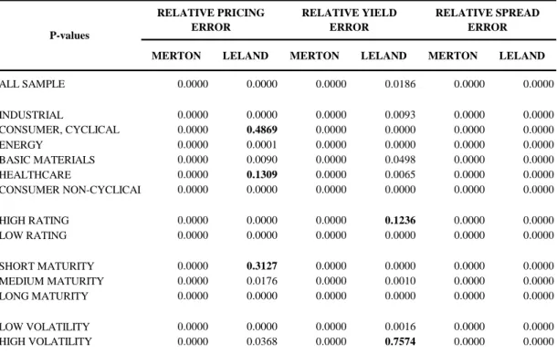
Parallel to the predicted errors presented in Table 3.4 we also test whether the mean relative errors are different from zero and whether there are differences between Merton and Leland means. Tables 3.5 and 3.6 report the p-values for these tests not only for the total sample which is analysed in this section but also for the grouping of relative errors according to sector, rating, maturity and asset volatility that is discussed in the next section.
Table 3.5 – P-Values to Test Mean Zero of the Relative Errors
Table 3.5 reports the P-values for a two-tailed test, which test the following hypothesis for the mean relative error. H0: µ = 0 and H1: µ ≠ 0. The values in bolt refer to cases where we cannot reject the null hypothesis that
the mean relative error is zero for a 5% significance level.
MERTON LELAND MERTON LELAND MERTON LELAND
ALL SAMPLE 0.0000 0.0000 0.0000 0.0186 0.0000 0.0000 INDUSTRIAL 0.0000 0.0000 0.0000 0.0093 0.0000 0.0000 CONSUMER, CYCLICAL 0.0000 0.4869 0.0000 0.0000 0.0000 0.0000 ENERGY 0.0000 0.0001 0.0000 0.0000 0.0000 0.0000 BASIC MATERIALS 0.0000 0.0090 0.0000 0.0498 0.0000 0.0000 HEALTHCARE 0.0000 0.1309 0.0000 0.0065 0.0000 0.0000 CONSUMER NON-CYCLICAL 0.0000 0.0000 0.0000 0.0000 0.0000 0.0000 HIGH RATING 0.0000 0.0000 0.0000 0.1236 0.0000 0.0000 LOW RATING 0.0000 0.0000 0.0000 0.0000 0.0000 0.0000 SHORT MATURITY 0.0000 0.3127 0.0000 0.0000 0.0000 0.0000 MEDIUM MATURITY 0.0000 0.0176 0.0000 0.0010 0.0000 0.0000 LONG MATURITY 0.0000 0.0000 0.0000 0.0000 0.0000 0.0000 LOW VOLATILITY 0.0000 0.0000 0.0000 0.0016 0.0000 0.0000 HIGH VOLATILITY 0.0000 0.0368 0.0000 0.7574 0.0000 0.0000 RELATIVE PRICING ERROR RELATIVE YIELD ERROR RELATIVE SPREAD ERROR P-values
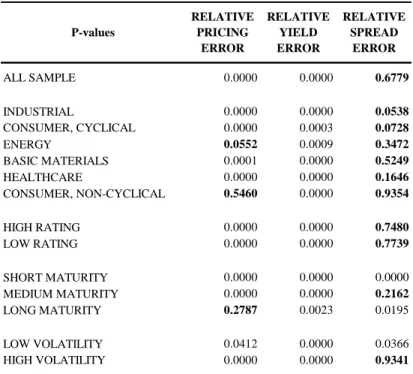
Table 3.6 – P-Values to Test Equality of Merton and Leland Means
Table 3.5 reports the P-values for a two-tailed test, which test the following hypothesis for the differences in Merton and Leland means relative errors. H0: µMerton - µLeland = 0 and H1: µMerton - µLeland ≠ 0. The values in bolt refer
to cases where the equality of means does hold for a 5% significance level.
The first conclusion that can be drawn from Table 3.4 is that both models overestimate bonds prices. Merton’s model mean overestimation is about 11.2% and Leland’s model is 4.5% (both means are significantly different from zero). The results found for the Merton model show an overestimation higher than the 4.5% found by Jones et al (1984) and 1.69% by Eom et al (2004). In this last case the author’s believe that the lower underestimation found in their study is due to the use of a payout ratio and a cost of financial distress in Merton’s model (Eom et al, 2004, p10). Not surprisingly, we found that Leland’s model overprices bonds less than Merton’s model (the equality of means does not hold for a 5% significance level). This is essentially due to the consideration of early default and cost of financial distress in Leland’s model.
Another important issue that should be discussed when analysing both models’ relative pricing errors is the distribution of these errors. These are depicted in Figure 3.3.
ALL SAMPLE 0.0000 0.0000 0.6779 INDUSTRIAL 0.0000 0.0000 0.0538 CONSUMER, CYCLICAL 0.0000 0.0003 0.0728 ENERGY 0.0552 0.0009 0.3472 BASIC MATERIALS 0.0001 0.0000 0.5249 HEALTHCARE 0.0000 0.0000 0.1646 CONSUMER, NON-CYCLICAL 0.5460 0.0000 0.9354 HIGH RATING 0.0000 0.0000 0.7480 LOW RATING 0.0000 0.0000 0.7739 SHORT MATURITY 0.0000 0.0000 0.0000 MEDIUM MATURITY 0.0000 0.0000 0.2162 LONG MATURITY 0.2787 0.0023 0.0195 LOW VOLATILITY 0.0412 0.0000 0.0366 HIGH VOLATILITY 0.0000 0.0000 0.9341 P-values RELATIVE PRICING ERROR RELATIVE YIELD ERROR RELATIVE SPREAD ERROR
Figure 3.3 – Distribution of Relative Pricing Errors
Panel A – Merton Panel B – Leland
Figure 3.3 provides evidence that the Merton distribution of relative pricing errors is skewed to the right while Leland’s distribution is just moderately skewed to the left. This reveals a tendency of the Merton model to overestimate bonds more than Leland’s model. Figure 5.3 also shows that there is a high dispersion of pricing errors, which is more pronounced in Leland’s distribution (standard deviation of 12.3% in Leland against 8.9% in Merton). In Leland’s model relative pricing errors range from –28% until 49%. This pattern of high dispersion is similar to the one found in previous literature. Eom et al (2004) report standard deviations of relative pricing errors of 4.94% in the Merton model (when the mean is 1.69%) and in other structural models most standard deviation of relative pricing errors are quite close to the mean (in level terms).
Regarding the yield and credit spread we notice, as expected, that both structural models underestimate these figures. The relative yield error is –30.5% and –3.4% for the Merton and Leland models, respectively, and the relative credit spread error is –76.2% and –75.0% also for both models, respectively (all means are different from zero). Again, we can compare the results for the Merton model with the Eom et al (2004) study. The results found for the yield relative error show less underestimation than Eom et al (2004). They found a relative yield error of –91.3% while our is only –30.5%. However, considering the relative spread error, the conclusion is somewhat different. Our mean of –76.2% shows more underestimation of credit spread than what they found: -54.4%.
The incapacity to generate sufficiently high spreads really seems to be one of the main critics of structural models. We might have several explanations for that. Some of them rely on technical issues and others on theoretical issues.
0 10 20 30 40 50 60 70 80 90 -27% -23% -19% -15% -11% -7% -3% 1% 5% 9% 13% 17% 21% 25% 29% 33% 37% 41% 45% More Relative Pricing Error
F re que nc y 0 10 20 30 40 50 60 70 -27% -23% -19% -15% -11% -7% -3% 1% 5% 9% 13% 17% 21% 25% 29% 33% 37% 41% 45% More Relative Pricing Error
F
re
que
nc
Regarding the technical issues, there seems to be a tractability problem. We cannot forget that both Merton and Leland models are approximating actual straight coupon bonds with finite maturity with some “Synthetic type of debt”. In Merton’s case it is a zero coupon debt and in Leland model its perpetual debt, with a continuous coupon payment. The calibration procedure used to convert “real debt” into “synthetic debt” will definitely imply different relationships between yields and prices in the model and in reality. That’s one of the reasons why “…a model which produces the correct price will not necessarily produce the correct credit spread (Ericsson and Reneby, 2002, p.14). The difference in model spread and actual spread – for the same bond price – may be several hundreds percent.
From a theoretical point of view, these structural models, which are based on the Contingent Claim Theory, tend to generate low credit spreads because they only capture the default risk component. Besides the credit risk component, actual credit spreads are very likely to include compensation for liquidity (marketability), taxes or systematic risk.
Among these three components, liquidity seems to have more influence in credit spread. Huang and Huang (2002) calibrate several structural bond pricing models to historical data in an attempt to estimate how much of the corporate bond yield spread is due to credit risk. They find that for investment grade bonds it constitutes no more than 20% of the overall spread, although this fraction is lower for more risky bonds.
The tax component of credit spread raises from the fact that, in some countries, namely in the U.S., a state income tax has to be paid on bond coupons and its principal at maturity and, as pointed out by Elton et al (2001), “corporate bonds have to offer a higher pre-tax return to yield the same after-tax return”. As regards the systematic component of credit spread, Collin-Dufresne et al (2001) identified that ¾ of credit spread changes are not explained by structural models but rather by systematic factors.
There is another feature related to “real” bonds that these two models do not capture: jumps in asset value. These models assume, as we explained in section 3, a geometric Brownian motion process for the asset value and, therefore, do not admit sudden changes (jumps) in the asset value. Even though these jumps are not so common in practice, there may be a small proportion of the market spread that compensates for jump risk not priced
When comparing Merton relative spread error with Leland’s relative spread error, we would expect a less negative error for the Leland model. Leland’s model not only considers the possibility of early default, which is an improvement of the Merton model and a closer approximation to reality, but also considers two “real world frictions”, namely taxes and bankruptcy costs. The Merton model assumes that upon default bondholders will recover 100% of the asset value while Leland’s model assumes a recovery rate that is less than 100%. By including these features, we would expect Leland’s relative spread error to be lower than Merton’s error. Nevertheless, this is not the case in our study. The p-value found for the equality of means (Table 5.6) is 0.6779, which reveals that we cannot reject the null hypothesis of equality of means (for a significance level of 5%).
Yet, as mentioned earlier, Leland’s calibration was more problematic than Merton’s because, during the sample period, the term structure was far from being flat and this might have some influence on the pricing results. Table 5.7 shows the sensitivity of Leland’s pricing, yield and spread errors to the risk free rate.
Table 3.7 – Leland Errors Sensitivity to the Risk Free Rate
Table 3.7 reports Leland’s absolute and relative predicted errors in price, yield and spread, as well as their standard deviation, for several levels of the risk free rate. Except for the first scenario, the risk free rate is computed using Nelson-Siegel (1987) risk free yield curve.
Focusing the analysis on the relative price error and the relative spread error (columns 4 and 8, respectively), we find that the lowest mean of the relative spread error
Absolute Error ($M) Relative Error Absolute Error (bp) Relative Error Absolute Error (bp) Relative Error Mean 10.3 4.5% -58.6 -3.4% -193.8 -75.0% Sd 36.4 12.3% 148.8 25.7% 140.2 31.1%
Risk free (T = 1) Mean -107.2 -29.4% -317.3 -52.0% -136.3 -43.4%
Sd 116.4 24.0% 132.3 14.6% 140.4 48.5%
Risk free (T = 5) Mean -22.3 -5.0% -192.9 -28.9% -170.4 -62.6%
Sd 59.3 16.2% 137.2 17.4% 140.0 39.0%
Risk free (T = 10) Mean 4.7 2.9% -90.4 -9.6% -189.1 -72.5%
Sd 40.6 13.0% 143.5 23.0% 140.2 32.7%
Risk free (T = 15) Mean 13.2 5.4% -35.8 0.8% -196.6 -76.4%
Sd 34.8 11.9% 149.1 26.9% 140.5 30.0%
Risk free (T = 30) Mean 13.6 5.5% -34.6 1.7% -196.7 -76.6%
Sd 33.9 11.8% 158.9 29.1% 140.3 30.2%
YIELD SPREAD
Risk Free implied in 60 semesters payment of $6.916M/2
LELAND MODEL All Firms
is obtained for a risk free rate corresponding to a maturity of one year, namely -43.4%. However, in this scenario, the relative mean pricing error presents a surprising result of -29.4%, revealing some contradiction with what we would expect from this structural model. This scenario is clearly unreasonable since we would be using a very short maturity risk free rate to discount perpetual coupons.
Another interesting figure is that, for a risk free computed for maturities above 10 years, the relative spread error shows low sensitivity to the risk free rate. The relative spread error only changes from –72.5% to –76.6% when we change the maturity of the risk free rate from 10 to 30 years. The relative mean spread error adopted for the dissertation (scenario one) is clearly in this range, which means that the fact that there are no differences between Leland’s and Merton’s relative spread errors estimation is not due to the choice of the risk free rate in Leland’s model.
Having compared the mean of Merton and Leland’s relative yield and spread errors, we shall now make some considerations about the distribution of these errors, as we did for the relative pricing errors. Figure 5.4 illustrates these distributions.
Figure 3.4 – Distribution of Relative Yield Errors and Relative Spread Errors
Panel A – Merton Relative Yield Error Panel B – Leland Relative Yield Error
Panel C – Merton Relative Spread Error Panel D – Leland Relative Spread Error 0 10 20 30 40 50 60 -75% -67% -59% -51% -43% -35% -27% -19% -11% -3% 5% 13% 21% 29% 37% 45% 53% 61% 69% More Relative Yield Error
F re que nc y 0 5 10 15 20 25 30 35 40 45 50 -75% -67% -59% -51% -43% -35% -27% -19% -11% -3% 5% 13% 21% 29% 37% 45% 53% 61% 69% More Relative Yield Error
F re q ue nc y 0 20 40 60 80 100 120 140 160 180 Fr eq u en cy 0 20 40 60 80 100 120 Fr eq u en cy
There is a clear distinction between the distribution of yield errors and the distribution of spread errors. While the distribution of yield errors has some similarities with a normal distribution, the distribution of spread errors shows an extreme concentration of observations in the lower bound. This pattern is more pronounced in Merton’s distribution. In this case there are 166 observations (52% of total) in the range –99% and –92%. But, at the same time, there are also some important observations with very positive spread errors: in the range above 44% there are 10 observations. This reveals the high dispersion of spread errors, usually a characteristic of these empirical studies. Even though we found a standard deviation of the relative spread error of 37% for the Merton model, Eom et al (2004) found a standard deviation even higher, namely 71.84%. Thus, these structural models have a tendency to predict either a very high spread or a very low spread.
The extreme underestimation demonstrated by these models requires a more detailed analysis of the observations. There are 35 observations for which the Merton model’s prediction spread is less than 1 bp, including 15 observations where the predicted spread is so close to zero that the prediction spread error is reported as –100%. On the other hand, in the Leland model, there is no prediction of spreads close to zero, which means that there are no reported errors of –100%. Still, there is a strong association between Merton and Leland’s predicted spreads, as the correlation between these variables is 0.92.
3.2.2 Predicted Errors By Category
In the previous section we discussed the performance of the structural models considering all the observations in the sample. However, there might be differences in the estimation errors according to the rating category of the bonds, its maturity or even the asset volatility of the firms. In this section we analyse the performance of the models according to this grouping and also according to sector.
To detect any rating effect, we divided the sample in two rating categories: high rating and low rating. High rating includes bonds with a numerical rating conversion below 11 (BBB-) and low rating all other bonds. This does not correspond to the standard distinction between investment grade bonds and speculative grade bonds (reported in Table 5.2) because there are only 32 observations of speculative grade bonds in the sample. It would not seem reasonable to compare results from a sub-sample of 32
observations with those from a sub-sample of 285 observations of investment grade bonds. The split resulted in 196 observations of high rated bonds and 121 of low rated bonds.
As regards the remaining time to maturity of the bonds, we analyse three sub-samples: short maturity (less than five years), medium maturity (from five to 10 years) and long maturity (above 10 years). It corresponds to 49, 169 and 99 observations, respectively. It would be interesting to analyse the ability of the models to generate reasonable spreads to very short maturities (<1 year) but, as mentioned in the data section, we exclude from our analysis corporate bonds with very short maturities as these are unlikely to be traded. That is the reason why we consider “short maturity” bonds with a remaining time to maturity of 3 and 4 years.
In order to discuss any volatility effects we decompose the sample in low asset volatility (below 20%) and high asset volatility (above 20%), which results in two sub-samples of 152 and 165 observations, respectively.
Table 3.8 gives the p-values of a two-way ANOVA test that evaluates, as a null hypothesis, no category effects according to rating, maturity of the bonds, asset volatility and sectors.
Table 3.8 – P-Values to Test No Category Effects According to Rating, Maturity, Asset Volatility and Sector
Table 3.8 reports the P-values for a two-way ANOVA test, which evaluates the following hypothesis for the means of relative errors in the Merton and Leland models.
H0: µHigh Rating = µLow Rating = 0 and H1: otherwise.
H0: µShort Maturity = µMedium Maturity = µLong Maturity = 0 and H1: otherwise.
H0: µ
Low Asset Volatility = µHigh Asset Volatility
= 0 and H1: otherwise.
H0: µIndustrial = µConsumer Cyclical = µEnergy = µBasic Materials = µHealthcare = µConsumer
Non-Cyclical = 0 and H1: otherwise.
The values in bolt refer to cases where there are not category effects for a 5% significance level.
MERTON LELAND MERTON LELAND MERTON LELAND
SECTORS 0.0000 0.0000 0.0000 0.0000 0.0000 0.0009 RATING 0.0000 0.0257 0.0000 0.0000 0.0464 0.0128 MATURITY 0.0119 0.0000 0.0000 0.0000 0.0000 0.1258 ASSET VOLATILITY 0.0000 0.0000 0.0040 0.0454 0.0000 0.0000 RELATIVE PRICING ERROR RELATIVE YIELD ERROR RELATIVE SPREAD ERROR P-values
Absolute Error ($M) Relative Error Absolute Error (bp) Relative Error Absolute Error (bp) Relative Error MERTON Mean 28.1 8.9% -155.3 -26.3% -155.3 -72.9% Sd 24.0 7.7% 144.3 18.7% 144.3 41.8% LELAND Mean 7.3 3.3% -23.4 3.0% -153.7 -71.6% Sd 35.7 9.7% 141.9 27.7% 125.9 35.1% MERTON Mean 34.2 14.8% -251.3 -37.3% -251.3 -81.5% Sd 26.8 9.6% 143.5 16.9% 143.5 28.7% LELAND Mean 15.1 6.5% -115.6 -13.8% -258.8 -80.6% Sd 37.3 15.4% 142.3 17.6% 138.4 22.2%
PRICE YIELD SPREAD
RATING MODEL
HIGH RATING
LOW RATING
Considering a 5% significance level, we reject the null hypothesis of no effects in Merton’s and Leland’s relative errors (pricing, yield and spread) according to rating, maturity, asset volatility and sector, except for the maturity in Leland’s relative spread error (p-value of 0.1258). To complement this analysis it is important to analyse the values of the relative predicted errors. Once again, we should analyse the magnitude of these errors in parallel with tables 5.5 and 5.6 which test the mean zero of the errors and the equality between Merton and Leland mean, respectively.
3.2.2.1 Rating
Table 3.9 displays the mean relative errors according to the rating category of the bonds. Both Merton’s and Leland’s models underestimate less the spread for high rating categories. Merton’s mean spread error is –72.9% for high rating bonds and –81.5% for low rating bonds. The p-value found for the equality between the Merton and Leland means (0.7480 for high rating and 0.7739 for low rating, Table 5.6) reveals that the equality of means does hold for spread errors.
Table 3.9 – Performance of the Structural Models According to Rating Category
Our findings are in accordance with what we should expect from the performance of the models. We should expect a lower capacity of the models to predict spreads of low rating bonds because low rating bonds are usually less liquid. Thus, their spread must show a bigger compensation for liquidity risk, which is not captured by structural models. These models only capture default risk.
A comparison to previous studies shows that our results contradict the results found by Ericsson and Reneby (2002). These authors report a better performance of the Merton
model for speculative grade bonds. However, Eom et al (2004) does not find significant differences of prediction between investment grade and speculative grade bonds for the Merton model.
3.2.2.2 Maturity
In the Merton model the tendency toward underestimation of spread appears to be somewhat stronger among short maturity bonds. We can observe in Table 3.10 that Merton’s relative mean spread error is –97% for short maturity bonds, -77.4% for medium maturities and –63.9% for long maturities. As the p-value of Table 5.8 shows, there is clearly a maturity effect in Merton’s spread prediction. In this case our results are in accordance with previous studies in the field, namely Ericsson and Reneby (2002) and Eom et al (2004).
Table 3.10 – Performance of the Structural Models according to Remaining Time to Maturity of the Bonds
We should note that for the Leland model the maturity effect of the relative spread error is not significant, as demonstrates the p-value of Table 5.8 (p-value of 0.1258).
3.2.2.3 Asset Volatility
Another interesting result from our study is that these structural models fit better prices and spreads of more risky firms (the p-values from Table 3.8 show a strong volatility
Absolute Error ($M) Relative Error Absolute Error (bp) Relative Error Absolute Error (bp) Relative Error MERTON Mean 24.5 8.0% -206.7 -40.7% -206.7 -97.0% Sd 16.8 6.6% 155.7 11.7% 155.7 6.8% LELAND Mean 1.4 0.9% 45.2 22.4% -184.3 -82.6% Sd 22.4 6.4% 175.8 34.4% 165.3 15.6% MERTON Mean 31.4 11.3% -229.4 -34.5% -229.4 -77.4% Sd 26.2 7.3% 159.6 19.5% 159.6 37.8% LELAND Mean 5.2 2.0% -70.5 -5.8% -225.5 -72.4% Sd 38.9 11.1% 147.2 22.9% 147.1 35.4% MERTON Mean 31.8 12.6% -120.7 -18.4% -120.7 -63.9% Sd 26.7 11.7% 102.6 13.7% 102.6 41.2% LELAND Mean 23.4 10.6% -89.6 -12.1% -144.5 -75.7% Sd 34.5 14.1% 111.8 15.0% 93.3 28.5% SPREAD SHORT MATURITY YIELD MATURITY MODEL PRICE LONG MATURITY MEDIUM MATURITY
effect). Table 3.11 reports these findings, which are similar to the ones found by Ericsson and Reneby (2002).
Table 3.11 – Performance of the Structural Models According to Asset Volatility of the Firms
Merton’s relative price error is 13.6% for low volatile firms and only 8.9% for high volatile firms. Concerning the spread, there is an extreme underestimation for low volatile firms, namely –93.4%, while for more risky firms this is only –60%. Leland’s results show some similarity, especially for the credit spread error. There is also empirical evidence that for high volatile firms the Leland model can fit with extreme precision the prices of the bonds. Leland’s relative pricing error for this category is significantly equal to zero (Table 5.5 reports a p-value of 0.7574 for a mean zero test, for a 5% significance level).
3.2.2.4 Sector
As far as we are concerned, there are no studies with an empirical analysis of the performance of these models according to sectors or industries. Thus, this constitutes one of the main contributions of this dissertation.
We already mentioned that there exists a sector effect in the performance of the models (in Table 3.8 the p-values for the equality of the means among sectors is zero for all errors). Now we will analyse which characteristics of the bonds or of the firms belonging to these sectors might lead to a better or worst performance of the structural models. Table 3.12 depicts the performance of the models according to sector.
Absolute Error ($M) Relative Error Absolute Error (bp) Relative Error Absolute Error (bp) Relative Error MERTON Mean 39.6 13.6% -202.9 -33.6% -202.9 -93.4% Sd 25.2 9.4% 125.4 13.3% 125.4 7.8% LELAND Mean 31.3 11.3% -72.4 -6.4% -196.2 -91.4% Sd 26.1 10.2% 138.2 25.0% 109.9 8.5% MERTON Mean 22.0 8.9% -181.9 -27.6% -181.9 -60.3% Sd 22.1 7.9% 171.4 22.3% 171.4 46.1% LELAND Mean -9.1 -1.7% -45.9 -0.6% -191.6 -60.0% Sd 33.8 10.6% 157.3 26.0% 163.6 36.4% ASSET VOLATILITY MODEL
PRICE YIELD SPREAD
LOW VOLATILITY
HIGH VOLATILITY
Table 3.12 – Performance of the Structural Models According to Sector
There are two sectors where the Merton model seems to perform better when predicting the credit spread: the Consumer Cyclical and the Energy sector. The relative spread errors have a mean of –58% and –62.5% in these two sectors, respectively, when the mean for the total sample is –76.2%.
By analysing Tables 2.1 and 2.2, which report descriptive statistics on the bonds and the firms according to sector, we verify that these sectors present some characteristics usually associated with a better prediction power of the Merton model. The bonds in the Consumer Cyclical sector have an average maturity above the average of the total sample and its firms also present asset volatilities and leverage levels above the total sample. We already tested that Merton model performs better for long maturity bonds and more risky firms. Regarding the leverage, the empirical literature shows that Merton’s model usually
Absolute Error ($M) Relative Error Absolute Error (bp) Relative Error Absolute Error (bp) Relative Error MERTON Mean 27.7 9.4% -180.3 -32.5% -180.3 -86.0% Sd 14.7 6.4% 108.4 14.0% 108.4 26.7% LELAND Mean 6.7 3.7% -2.7 7.3% -170.9 -77.6% Sd 27.4 7.1% 135.8 28.0% 109.5 33.4% MERTON Mean 27.8 10.7% -162.1 -22.3% -162.1 -58.0% Sd 27.9 9.8% 178.0 19.7% 178.0 41.8% LELAND Mean 4.4 1.3% -96.5 -10.8% -203.2 -68.9% Sd 44.4 15.0% 146.1 15.9% 166.9 25.5% MERTON Mean 42.8 10.6% -135.2 -21.8% -135.2 -62.5% Sd 37.6 8.3% 115.8 18.0% 115.8 43.1% LELAND Mean 27.2 6.5% -69.0 -10.1% -150.3 -70.2% Sd 45.1 11.3% 88.5 13.6% 100.1 33.2% MERTON Mean 31.4 12.5% -275.1 -37.7% -275.1 -80.6% Sd 27.1 8.3% 213.5 23.3% 213.5 47.0% LELAND Mean 4.7 4.1% -97.6 -7.8% -251.2 -74.6% Sd 36.8 10.2% 179.7 25.9% 189.6 40.2% MERTON Mean 18.1 6.8% -143.0 -29.3% -143.0 -77.1% Sd 11.9 4.4% 81.4 16.5% 81.4 33.7% LELAND Mean -5.4 -2.5% 41.5 14.7% -118.8 -66.8% Sd 24.2 9.5% 102.0 31.1% 65.4 24.9% MERTON Mean 38.4 20.5% -302.5 -43.9% -302.5 -95.1% Sd 23.6 12.0% 101.3 12.6% 101.3 5.8% LELAND Mean 33.1 18.6% -184.1 -24.1% -301.6 -95.0% Sd 20.1 13.7% 121.5 14.0% 98.8 4.2%
PRICE YIELD SPREAD
HEALTHCARE CONSUMER, NON-CYCLICAL MODEL SECTOR INDUSTRIAL CONSUMER, CYCLICAL ENERGY BASIC MATERIALS
we believe that the good performance of the Merton model is probably due to the highest average time to maturity of its bonds (14.2 years for an overall average of 9.7 years).
In the group of sectors with worst predictive power of the Merton model we found the Consumer Non-Cyclical and the Industrial with relative spread errors of –86% and –95%, respectively. The poor performance in the Industrial sector seems to be due to the short average maturity of its bonds (5.8 years, which is the lowest of the sample) and the low asset volatility of its firms. As regards the Consumer Non-Cyclical sector it seems to be due to the reduced asset volatility of its firms.
The p-values presented in Table 3.6 from the test of equality of means between Merton and Leland models show that there are no differences in these means regarding the spread prediction of the six sectors (for a 5% significance level).
In relation to the relative price error among sectors we should note the excellent performance of the Leland model in the Consumer Cyclical and Healthcare sectors, as the mean of this error is statistically zero, considering a 5% significance level (p-value of 0.4869 in the Consumer Cyclical sector and 0.1309 in the Healthcare sector, as reported in Table 3.5).
We can summarize the analysis of the predictions errors as follows. Both Merton and Leland models overestimate bond prices and underestimate credit spreads. Even though in the spread predictions the results are not statistically different from each other, in the prices predictions Merton’s overestimation is stronger. We also confirm Eom et al (2004) results of high dispersion of credit spread errors. The analysis of the prediction errors by category show that both Merton and Leland’s models perform better for bonds with a good rating quality and a longer maturity. Moreover, these models perform better with riskier firms, those that present high asset volatility and high leverage.
3.3 Systematic Prediction Errors
Up to this point we have discussed the performance of the structural models analysing essentially some descriptive statistics of the predicted errors in terms of pricing, yield and spread. We considered the mean relative spread error to be the most informative measure of the ability of the models to fit credit spreads. In this section, we consider in more detail the question of why the models’ predictions are inaccurate. With a multivariate regression analysis we examine the relationship between the relative spread error and a set of bond specific, firm specific and economy wide variables. The goal is to identify some systematic factors that cause the weaknesses of the models. This analysis covers the entire sample as well as several categories of rating, maturity, asset volatility and sector.
The methodology used in this section is somewhat similar to the methodology used by Eom et al (2004), Ericsson and Reneby (2002) and Lyden and Saraniti (2000). All these authors perform a multivariate regression analysis instead of a single regression analysis. They argue that a combination of factors leads to higher or lower prediction errors and, therefore, analysis in a multivariate regression setting is more appropriate.
Nevertheless, there are some differences in the choice of the dependent variable. Eom et al (2004) use the relative spread error as the dependent variable while Ericsson and Reneby (2002) and Lyden and Saraniti (2000) use the absolute spread error. But, even the spread error is not defined in the same way by all these studies. While the first two use the definition of error as we do, Lyden and Saraniti (2000) use an inverse definition, which leads to positive errors for these models4. Following the most recent empirical paper in the field, the one by Eom et al (2004), we use the relative spread error as dependent variable, which makes our findings directly comparable to this study.
In the list of explanatory variables we consider size, leverage, asset volatility, market-to-book ratio and stock return as firm specific variables. We use the market value of assets as a proxy for size. Leverage is the market leverage, defined as the ratio of the sum of market value of trade debt and book value of non-traded by the market value of assets. We use the definition of market-to-book ratio presented by Rajan and Zingales (1995) as the ratio of market value of assets to book value of assets. This variable in intended to
Credit Spread
Merton RSE
Leland
RSE Size Lever. Yrs to Mat. Asset Volatil. Rating MB Ratio Stock Return Obs. YTM Level of TS Slope of TS Credit Spread 1.00 Merton RSE -0.01 1.00 Leland RSE -0.11 0.87 1.00 Size -0.31 0.12 0.31 1.00 Leverage 0.33 0.14 -0.07 -0.17 1.00 Yrs to Mat. -0.18 0.18 -0.05 -0.08 0.06 1.00 Asset Volatility 0.20 0.60 0.67 0.08 -0.43 -0.15 1.00 Rating 0.56 -0.01 -0.12 -0.33 0.26 -0.13 0.11 1.00 MB Ratio -0.19 -0.12 0.03 0.18 -0.64 -0.14 0.32 -0.11 1.00 Stock Return -0.11 -0.31 -0.35 0.06 -0.21 0.11 -0.25 -0.05 0.24 1.00 Obs. YTM 0.84 0.11 -0.08 -0.31 0.30 0.20 0.21 0.46 -0.21 -0.02 1.00 Level of TS 0.12 0.06 0.00 -0.02 -0.08 0.10 0.17 0.00 0.06 0.12 0.51 1.00 Slope of TS -0.26 -0.06 -0.01 0.04 0.07 -0.11 -0.20 0.00 -0.03 -0.05 -0.55 -0.63 1.00 stand for the firm’s growing opportunities. The stock return is computed as the annualised stock return of the last 250 days prior to the quarter considered for each firm.
We also evaluated whether we should consider the tangibility of a firm’s assets in the list of firm specific variables. As proposed by Rajan and Zingales (1995), the tangibility can be approximated by the ratio of fixed assets to total assets. However, we decided not to include this variable as it presents a strong association with leverage, one of our explanatory variables. The inclusion of both variables could create multicollinearity problems in our regressions.
As bond specific variables we use the remaining time to maturity of the bonds, the rating (again with the numerical conversion of Table 5.2) and the observed yield to maturity. Since each regression is estimated using bond prices observed in a variety of interest rate environments we consider two control variables related to term structure. The ten-year yield is used to measure the level of the term structure and the difference between the ten and two year yields to measure the slope. In order to have a first picture of the relationship between the variables used in the regressions, we present below the correlation matrix.