Optimal design and controlof mechanical systems with uncertain input

DOI 10.3233/SAV-2012-0708 IOS Press

ISSN 1070-9622/12/$27.50 © 2012 – IOS Press and the authors. All rights reserved

Optimal design and control of mechanical

systems with uncertain input

P.P. Moita

a,

*, J.B. Cardoso

b

and A. Barreiros

b

a_{Escola Superior de Tecnologia, Setúbal, Portugal}

b_{Departamento de Engenharia Mecânica, Instituto Superior Técnico, Lisboa, Portugal}

Abstract. This paper presents an integrated approach to optimize for design and control of mechanical systems with random

input parameters. Random parameters are represented by probability density functions. A numerical technique defining directly the representative values and the associated probabilities is implemented by modeling the stochastic parameters as generalized Wiener processes. The Monte Carlo’s method is also implemented to deal with correlated parameters. A design and control sensitivity analysis optimization formulation is derived. A conceptual separation between time variant and time invariant design parameters is presented, this way including the design space into the control space and considering the design variables as control variables not depending on time. By using time integrals through all the derivations, the design and control problems are unified. In the optimization process we can use both types of variables simultaneously or by interdependent levels. The dynamic response is modeled via space and time finite elements, and is integrated either by at-once integration or step-by-step. The formulation is applied to a numerical example.

Keywords: Space-time finite elements, adjoint system, stochastic modeling, wiener processes

1. Stochastic modeling

Most of the optimum design is applied to systems under deterministic loading. However, much of the decision making in real world deals with systems that may not be precisely described. When the system parameters are described as random variables through statistics as mean and standard deviation, a probabilistic approach can be used for the analysis and design of the system [8]. This paper presents an approach to optimize for designing of mechanical systems with random input parameters. The random parameters are characterized by specifying their probability density functions.

Due to their multivariate nature, integrations involving these functions are in general impracticable. However, this limitation may be overcome by adopting a methodology that makes possible to substitute the continuous dis-tributions by discrete disdis-tributions with identical expected values and covariance matrices. In this methodology, the random parameters are described by generalized Wiener processes.

At the present state of the research work, we consider that only the dimensions of the obstacles encountered by the system are random. The location of the obstacles is assumed deterministic.

Under these conditions, the value g of the obstacles is obtained from one of the following stochastic differential equations:



,



dg  W   d  dW (1)



,



dg  W g d  g dW (2)

*Corresponding author: P.P. Moita, Escola Superior de Tecnologia, Campus do IPS, 2914-508, Setúbal, Portugal. E-mail: paulo.moita@ estsetubal.ips.pt.

where  and 2are constants, W represents a Brownian motion and



is the time. The time here is an auxiliary variable that represents the point from which the dimensions of a given obstacle have been grown continuously up to the present value.

The first process leads to a Gaussian distribution while the second one leads to a Log-Normal distribution. We assumed that the obstacles have only positive dimensions and adopted the second equation, which has the following solution:



2



0exp 2

g g _

 



 

 W_ (3)

The expected value and the variance of g are then given by:

 

0 exp





E g g  (4)

 

 

2 _exp



2



₁

Var g_ E g_ _    _ (5)

From these equations, the parametersand 2can be obtained by specifying the expected value and the vari-ance of g.

To obtain the discrete distribution, the temporal evolution of the logarithm of g was simulated using trinomial movements [9]. The use of this transformation is justified due to its advantage of leading to constant elemental probabilities of evolution. The corresponding process is obtained using the Ito’s lemma [10] and it is represented by the following equation:

df   d  dW (6)

where   2 2andf ln( )g . Since the first and second moments of the continuous and discrete distribu-tions coincide, the following equadistribu-tions for the probabilities are obtained as [3,4]:





2 2 u d d d u t f P f f f           (7)





2 2 1 u d m d u t f f P f f            (8)





2 2 d u u d u t f P f f f           (9)

where the parameters involved are represented graphically in the Fig. 1.

Fig. 1 Trinomial evolution of the stochastic variable

where  E



f

 

 f_mf_t



, f_d  f_mf_dand fu  fu fm. The values of f can be chosen using the condition of identical probabilities and the value of t determines the number of points obtained. Using a uniform

) (t t f t ft d f m f u f  fu d f  ) (tt ) (t t f t ft d f m f u f  fu d f  ) (tt

grid and several time steps, the probabilities of the ending nodes can be obtained applying the following recurrence relation: 1 1 1 1 1 t t t t u m d i i i i P P P_ P P P P_ (10)

Finally, after the definition of this distribution, the value of an obstacle dimension at a given location has been obtained by selecting randomly one of those values using the accumulated probabilities (i.e. the distribution func-tion) and a corresponding random value obtained from a uniform distribution between 0 and 1.

2. Analysis and design sensitivity analysis modeling

For the dynamic response analysis and design sensitivity analysis, space and time finite element discretizations are included in the same system of equations [11] such that space and time integrations can be performed simul-taneously by at-once integration as for static cases. Design sensitivity analysis is implemented throughout the ad-joint system approach [5].

2.1. Analysis

A space-time finite element model is used to discretize the dynamic analysis response. After space discretization we have the governing matrix equation as

t t t t t t

S S

M U + C U + K U = P (11)

where M is the mass matrix,tCS tCS(tU), tKS tKS(tU are respectively the damping and stiffness matrices, ) t_{P is the loading vector and}

,

t_{U, U U}t t _{are respectively the displacement, velocity and acceleration vectors, all the} quantities defined at time t.

For temporal modeling, finite elements of dimensiontwere considered, selecting hermitean cubic elements to model the displacements and quadratic lagrangean elements to model the loading, extending the algorithm given in [7] to the case of nonlinear systems. By taking the time derivative of the Eq. (11) by one hand, and by another hand its integration once and then twice with average values of stiffness and damping given as

2 ₂ 2 ₂ t t t t t t t t S( t ), S( t )  _  _     K K U + U C C U + U (12)

one obtains four equations that combine to give the dynamic finite time-element equation as

e e e S  D z P (13) where 11 12 11 12 21 22 21 22 , t t t S S nxn nxn nxn e t t t t t t e S S S nxn S S nxn 1 t t t t t t S S nxn S S nxn 2               _ _    _{  }   _{ }   _{ }     K C M P D D D D D P P D D D D P 0 0 0 0 0 0 0 (14) and ( , ), ( , ) e _ t tt t _ t t t z z z z U, U U (15)

The Eq. (13) may be solved step-by-step, i.e., element-by-element in time, or assembled to be solved at-once. In this case, we have to assemble for a total time interval T discretized in N time nodes, resulting in the dynamic equation

S 

D z P (16)

where 2n time boundary conditions are imposed by transferring the corresponding columns of the assembled matrix

S

D to the right-hand side of Eq. (16) after multiplying by the vector Ucof those conditions, resulting the equation ˆ ˆ_{S } ˆ_, ˆ _{  c c}

K U P P P D U (17)

The Eq. (17) is a nonlinear equation where ˆK is a nonsymmetrical matrix dependent on the response _S Uˆ . Therefore, the Eq. (17) has to be solved iteratively.

2.2. Design sensitivity analysis

Consider now a general performance measure defined in the interval [0,T] as (t t )

G , , t dt

 

_

z b (18)

wheretbis the vector of design and control variables and tzis the state vector already defined in Eq. (15). The external forces t_{P generally belong to the design vector.}

The design sensitivity analysis problem is to derive the total design variation of the measure in Eq. (18) with respect to the design tb, for the system represented by the equation of motion, Eq. (17).

The total design variation for the performance measure of Eq. (18) is



    





(19)

where



and  represent respectively the explicit and implicit (state dependent) design variations.

In order to formulate the adjoint system method, replace the arbitrary variation of state fields by adjoint fields into the virtual work equation as

ˆ ˆ ˆ ˆ ₀

a a

S

W = K U - P U( )  (20)

and define an extended ‘action’ function a

A  W (21)

The basic idea of introducing an adjoint system is to replace the implicit design variations of the state fields by explicit design variations and adjoint fields to be determined by imposing the implicit design variation of the ‘action’ function A to vanish,

0 A

  (22)

then the total design variation can be written as A



 



(23)

In order to solve the design sensitivity analysis problem, the sensitivities are firstly performed at the element level and then the sensitivity equations are assembled. The explicit design variation of the vector of element forces of Eq. (13) is

,

e e e e e e

S

R P F F D z (24)

and the implicit design variation of the internal forces gives

e e e e e e e S S F D z D z D z (25) where 11 12 11 12 21 22 21 22 t t nxn nxn nxn e t t t t t t nxn nxn t t t t t t nxn nxn                      K C M D D D D D D D D D 0 0 0 0 0 0 0 (26) with , , , , t t t t t t t t S S S S t t t t t t jk Sjk Sjk Sjk ,    U U U U K = K K U C = C C U D = D D U + D U (27)

Sensitivities of Eq. (24) and the element dynamic matrix of Eq. (26) are assembled and again imposed the time boundary conditions resulting respectively RˆandKˆ .

Now, the application of the Eq. (22) to the Eq. (21) gives the adjoint system equilibrium ˆ

ˆ ˆT a _{ ( , )}T

U

K U (28)

Then, the total design variation of Eq. (23) is ˆa ˆ

    U R (29)

3. Example

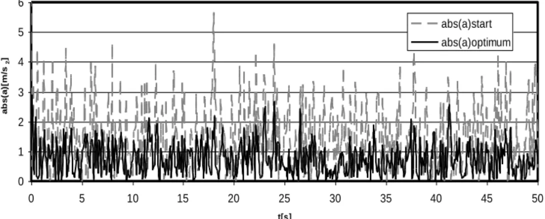
A simple one degree of freedom system of unit mass is subject to a stochastic kinematic excitation specified by a maximum expected value of 50 mm and a maximum variation of 0.25 mm for the perturbation displacement. Considering the average absolute value of the acceleration along the time T as the optimality criterium, say

1 , avg

a T  u dt the system is optimized with respect to the spring and damping characteristics, respectively the stiffness K and the damping C. By using a Wiener process and trinomial trees of five steps, 12 point obstacles of different heights and probabilities of occurrence are determined. These obstacles are randomly distributed by Monte Carlo´s method, according to the respective frequency of occurrence, along a time interval of T = 50 s, separated of each other by 0.05 s, originating 1000 random obstacles, defining a kinematic input. Additionally, five diferent Monte Carlo simulations were run for the same maximum expected value and maximum variation of the input. This way, we generated five different sets of obstacles.

The starting design variables were prescribed as K = 100 N/m and C = 10 N.s/m. With these values one achieves an objective of 1.3375 a_avg 1.4497m/s2. The optimum values of the design variables are estimated as

*

91.93 K 94.76N/m, 92.68 C* 101.3N.s/m by using a recursive quadratic algorithm. The optimum ob-jective is estimated as 0.97553 aavg* 0.99161m/s2 with a mean value of 0.97665 m/s2, and a standard deviation of 0.014294 m/s2, resulting a save at least of about 35%. In Fig. 1 one can see the starting and the optimum accel-eration response for one the Monte Carlo simulations.

The optimization runs were then repeated with T = 100 s, instead of T = 50 s and the same time separation be-tween obstacles, this way doubling its number. The mean and standard deviations of the average acceleration ob-tained for that second run of the optimizations were 0.95979 m/s2 and 0.014676 m/s2, respectively. The small dif-ferences obtained lead us to conclude that the number of obstacles in the first run was already high enough to eliminate the influence of the number of obstacles in the optimization results.

4. Remarks

This paper presents an approach to optimize for designing of mechanical systems with random input parameters, wher these parameters are characterized by specifying their probability density functions. As the integration of these functions is generally impracticable, a methodology is applied, where random parameters are described by gener-alized Wiener processes, such that it makes possible to substitute the continuous distributions by discrete distribu-tions with identical expected values and covariance matrices. The system kinematic input is simulated by obstacles which dimensions are random. The obstacles distribution in time is simulated by using Monte Carlo’s method. The optimization runs are performed accordingly to the Monte Carlo simulations, obtaining optimum values that im-prove effectively the objective function. For the optimization process, the design sensitivity analysis has been performed by using the adjoint system method. As the dynamic equations are integrated “at-once”, this method does not have the same drawbacks as it has in the case of “step-by-step” integration, namely the need of memorizing the entire analysis response.

Fig. 2. Starting and optimum acceleration response for one the Monte Carlo simulations.

References

[1] J.S. Arora and T.C. Lin, A Study of Augmented Lagrangean Methods for Simultaneous Optimization of Controls and Structures, Fourth AIAA/Air Force/NASA/OAI Symposium, Cleveland, Ohio, USA, 1992.

[2] J.S. Arora, Introduction to Optimum Design, McGraw-Hill, 1989.

[3] A. Barreiros, Probability Density Functions for Stochastic Linear Programming, Proc. of CCCT'04, Austin, USA, 2004.

[4] A. Barreiros, Optimization Under Stochastic Linear Programming, 6th World Congress on Structural and Multidisciplinary Optimization, Rio de Janeiro, 30 May–3 June, 2005.

[5] J.B. Cardoso and J.S. Arora, Design sensitivity analysis of nonlinear dynamic response of structural and mechanical systems, Structural

Optimization 4 (1992), 37–46.

[6] J.B. Cardoso and J.S. Arora, Variational method for design sensitivity analysis in nonlinear structural mechanics, AIAA Journal 26(5) (1988), 595–603.

[7] M. Gellert, A new algorithm for integration of dynamic systems, Computers & Structures 9 (1978), 401–408.

[8] L. Howell, S.S. Rao and A. Midha, Reliability-based optimal design of a compliant mechanism, ASME Journal of Mechanical Design 116 (1994), 1115–1121.

[9] J. Hull, Options Futures and Other Derivative Securities, Prentice-Hall, 1993.

[10] F.C. Klebaner, Introduction to Stochastic Calculus with Applications, Imperial College Press, 1998.

0 1 2 3 4 5 6 0 5 10 15 20 25 30 35 40 45 50 t[s] a b s (a )[ m /s 2 ] abs(a)start abs(a)optimum

[11] P.P. Moita, J.B. Cardoso and A.J. Valido, A space-time finite element model for control and design optimization of nonlinear dynamic response, Journal of Shock and Vibration 15(3,4) (2008), 307–314.

[12] E. Polak, On the use of consistent approximations in the solution of semi-infinite optimization and optimal control problems,

Mathe-matical Programming 62 (1993), 385–415.

[13] M. Salama, J. Garba, L. Demsetz and F. Udwadia, Simultaneous optimization of controlled structures, Computational Mechanics Mech 3 (1988), 275–282.

[14] J.C. Spall, Introduction to Stochastic Search and Optimization: Estimation, simulation, and Control, John Wiley, 2003.

[15] C.H. Tseng and J.S. Arora, Optimum design of systems for dynamics and controls using sequential quadratic programming, AIAA Journal

27(12) (1989), 1793–1800.

[16] Y.M. Zhang, Dynamic research of a nonlinear stochastic vibratory machine, Shock and Vibration 9 (2002), 277–281.

[17] J. Hlaváček, Chleboun and I. Babučka, Uncertain Input Data Problems and the Worst Scenario Method, Elsevier, Amsterdam, 2004. [18] R. Sampaio and E. Cataldo, Comparing two strategies to model uncertainties in structural dynamics, Shock and Vibration 17 (2010), 171–

multiple sites or posted to a listserv without the copyright holder's express written permission. However, users

may print, download, or email articles for individual use.