Lat. Am. j. solids struct. vol.8 número4

(1)

Optimization of laminated composite plates and shells using

genetic algorithms, neural networks and finite elements

Abstract

Structural optimization using computational tools has be-come a major research field in recent years. Methods com-monly used in structural analysis and optimization may de-mand considerable computational cost, depending on the problem complexity. Therefore, many techniques have been evaluated in order to diminish such impact. Among these various techniques, Artificial Neural Networks (ANN) may be considered as one of the main alternatives, when com-bined with classic analysis and optimization methods, to reduce the computational effort without affecting the final solution quality. Use of laminated composite structures has been continuously growing in the last decades due to the ex-cellent mechanical properties and low weight characterizing these materials. Taken into account the increasing scien-tific effort in the different topics of this area, the aim of the present work is the formulation and implementation of a computational code to optimize manufactured complex lam-inated structures with a relatively low computational cost by combining the Finite Element Method (FEM) for structural analysis, Genetic Algorithms (GA) for structural optimiza-tion and ANN to approximate the finite element soluoptimiza-tions. The modules for linear and geometrically non-linear static fi-nite element analysis and for optimize laminated composite plates and shells, using GA, were previously implemented. Here, the finite element module is extended to analyze dy-namic responses to solve optimization problems based in fre-quencies and modal criteria, and a perceptron ANN module is added to approximate finite element analyses. Several ex-amples are presented to show the effectiveness of ANN to approximate solutions obtained using the FEM and to re-duce significatively the computational cost.

Keywords

laminated composite plates and shells, artificial neural net-works, optimization, genetic algorithms, finite element

Sergio D. Cardozo∗_,

Herbert. M. Gomes and Armando. M. Awruch

Graduate Program in Mechanical Engineering, Federal University of Rio Grande do Sul, Rua Sarmento Leite, 425, 90050-170 Porto Alegre, RS – Brazil

Received 17 Mar 2011; In revised form 30 Sep 2011

(2)

1 INTRODUCTION

The structural optimization is not a new field. Galileo in his text “Discorsi e Dimostrazioni Matematiche intorno a due Nuove Scienze” (1638) studied the problem which consists of finding the shape of a beam where every transversal section has the same stress distribution.

In composite materials structures, some experiences has shown that Genetic Algorithms (GA) perform better than traditional gradient based techniques due to the discrete nature of the design variables.

A problem that arises when GAs are used is the high computational cost demanded by this method. For this reason some techniques to reduce this cost have been tested. One of them, consists of replacing the complete Finite Element Analysis (FEA) by some approximation technique. The Artificial Neural Network (ANN) have been shown to be a good alternative to avoid the large number of FEA involved in a GA.

In this work these two techniques are combined to make the process faster and cheaper in terms of computational cost.

This work is based on [2], from which some GA parameters, objective functions and results are taken in order to compare the effectiveness of substituting a complete FEA by ANN.

2 STRUCTURAL OPTIMIZATION

The structural optimization can be understand as a process to search the configuration which gives the best performance, within some criteria and subjected to certain design constraints.

To model the structural optimization as a mathematical optimization problem, the follow-ing concepts are used:

• Design variables: they are the characteristics that can be modified by the mathematical

optimization algorithm to obtain the best structural performance.

• Design constrains: are the restrictions applied to the structure, such as a limit to avoid

material failure, maximum or minimum value of design variables and others that depend on the problem being analyzed.

• Objective function: it is a mathematical expression in which the design variables and

constrains are involved. This function represents a number which has to be maximized or minimized during the optimization process.

2.1 Structural analysis

The analysis of the composite structures is carried out using the FEM. The element used is a triangular flat plate bending element with 18 degree of freedom called DKT (Discrete Kirchhoff Triangle) combined with the CST (Constant Strain Triangle) to take into account membrane effects. This element was developed by [3] for isotropic materials and it was extended by [1] for laminated composite materials.

(3)

To solve geometrically non linear problems, the generalized displacement control method (GDCM) described by [12] is used.

The Tsai-Wu failure criterion is employed for failure prediction in a ply see [4].

2.2 Genetic algorithms for composite materials

Genetic Algorithm (GA) is a computational search tool based on concepts of natural selec-tion and survival of the fittest individual. One aspect of fundamental importance in GAs is the way the solutions are tracked. Instead of using derivatives or gradients, as in determin-istic optimization algorithms, GAs work with the objective function based on simple values of individuals. This feature makes the method suitable for problems involving discontinuous functions, and/or non-defined derivatives like in integer programming. Moreover, unlike de-terministic optimization methods, which perform the search focusing on a single solution at a time, the GAs work with a population of individuals in each generation. Thus, as several search points are maintained, the convergence or stagnation to local minima, if the starting point is poorly chosen, is prevented. All these aspects result in more chances of finding the optimal solution, even on problems having hard search spaces with multiple local minimum [5].

The design of the optimal sequence of layers in laminated composite materials is a problem of global minimum. Due to the stochastic characteristics of GAs, they are more suitable to optimize than deterministic methods of optimization, which often converge to solutions representing a local minimum. Moreover, in commercial designs, fiber orientation angles and the amount and thickness of layers are discrete variables, a fact which confirms the suitability of GAs for these kinds of problems.

More details related to the use of the method for optimization of composite structures can be found in [2], [9] and [10].

The GA approach adopted here was proposed by [11] and extended by [1]. The classi-cal GA is modified to manage composite materials structures. Two genes are used, one for materials and another for the orientation of reinforcement fibers on each ply. The genetic operations used here are crossover, mutation and gene swap. The selection scheme adopted is the Multiple Elitist 1 proposed by [11]. In this scheme some of the best individuals from the parents and sons generations are used in the son generation to maintain and to improve the evolution. Ne is defined as the number of individuals of each generation. The criterion to stop the GA is defined by two parameters. The first one is the number that limits the number of generations (NLG), which is used to limit the total number of generations in the GA. The second one, is the number of generation with the same optimum design (NSD), which indicates that the convergence rate has been zero for a defined number of generations.

3 ARTIFICIAL NEURAL NETWORKS

(4)

use of ANN to predict structural responses has been growing in recent years. To continue this research line here, neural networks will be applied to learn the structural response of laminated composite structures. The neural network model used here is briefly described below. More details may be found in [6].

3.1 Multilayer perceptrons

A general Multilayer Perceptron Network (MPN) architecture consists on a layered network fully connected, i.e., all neurons belonging to a layer are, each one, connected to the previous and the next layer. Such architecture representation is indicated by the number of input vector followed by the number of neurons on each layer and the output vector (e.g. 1:12:1 indicates an Artificial Neural Network with one input vector, followed by one hidden layer with 12 neurons and an output layer with one neuron).

The ANN Architecture depends on the complexity of the system being modeled. For a more complex system, a larger number of hidden units are needed. In the training process of neural networks, for an input pattern Xpi (where index p means “pattern” and index i means an input neuron), the weight (wpi) adjustments will take place in the links of the neural network in order to get a desired outputOpkclose to the function which are being fittedYpo(omeans an output neuron). For each input-output pattern, the square of the error and the average system error should be minimized. They may be written, respectively, as Ep=

1

2∑k(Ypk−Opk) 2

and E = 1

2∑pEp, where k is the number of neurons in the output layer, and p is the number of training patterns. Employing any algorithm to minimize the error function, the weights can be evaluated and an approximated fit may be obtained. The standard back-propagation algorithm is used to adjust the different weights as well as the derivatives ofOpk with respect to the input data which will be fitted. After this first adjustment takes place, the network will pick up another pair of Xpi and Ypo, and will again adjust weights for this new pair. In a similar way, the process will go on until all the input-output pairs are considered. After some training epochs, the network will have a single set of stabilized weights satisfying all the input-output pairs with an average system error lower than a tolerance (10−3

). More details regarding the use of the MPN can be found in [7] and [6].

3.2 Artificial neural networks and genetic algorithms

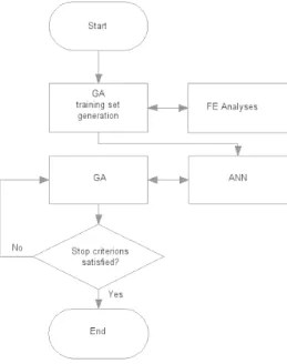
To combine the ANN and GA, the scheme shown in Fig. 1 is adopted. To generate the training set for the ANN in each case, three GA are executed with two generations having large populations each one. This approach is used to make a randomly distributed generation in the first one and some elitist generation in the second one. Three executions of the GA make the generations disperse and they are enough to guarantee that almost every zone of the design space is covered.

(5)

Figure 1 Flowchart of GA-ANN.

4 NUMERICAL EXAMPLES AND DISCUSSION

To evaluate the quality of the optimization scheme and the time that can be saved using ANN, three examples are shown. In each one, the GA and the training time as well as the error of the ANN (with respect to the Finite Element Method (FEM) solution) are presented, together with a comparison of GA-FEM with respect to processing time and quality of results are also presented. All examples have been executed in a 2.4 Ghz Quad Core 2 computer with 4 Gb of RAM.

4.1 Cost and weight minimization of an in-plane loaded composite laminated plate

In this problem the number of plies, the material of each ply and the orientation of reinforce-ment fibers are the design variables. The right combination of these variables can determine the cheapest and lightest structure. The constraints of the problem are the material failure (λf) derived from the Tsai-Wu criterion [4], and the structural elastic stability (λb). Both must be greater or equal to 1.0. The cost is proportional to the material consumption in the laminated structure, and each material has its own cost per unit weight denoted by C. The plate model with boundary and load conditions is shown in Fig. 2. The finite element mesh has 3000 elements. The objective function is defined by Eq. 1 , where W t∗ _and _C∗ _{are the}

(6)

Figure 2 Composite laminated plate with its boundary and load conditions.

⎧⎪⎪⎪⎪ ⎪⎨ ⎪⎪⎪⎪⎪ ⎩

OBJ =10₋ √

[φ(W t∗)2]

2

+[(1−φ) (C∗)2]

2

+10−6λ∗ , if λ∗≥1

OBJ =(λ∗)2{₁₀ −

√

[φ(W t∗)2]

2

+[(1−φ) (C∗)2]

2

} , if λ∗_<₁

(1)

C∗₌ C−Cmin Cmax−Cmin +

1 W t∗₌ W −Wmin Wmax−Wmin +

1 λ∗₌_minimum(_λ

f, λb) (2)

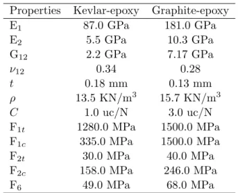
The elastic constants, strength parameters, specific weight, ply thickness and the parameter of cost per unit weight for the Kevlar-epoxy and Graphite-epoxy are shown in Table 1. The elastic constants are the Young’s modulus in the fiber direction (E1) and transverse to the fiber direction (E2), the shear modulus (G12) and the Poisson’s ratio (ν12), respectively. Strength parameters for tension and compression for longitudinal and transversal directions are given byF1t,F1c,F2t, andF2c, respectively. The remainder parameters are the shear strength (F6), the specific weight (ρ) and the thickness (t).

The alphabet used in the GA is shown in Table 2; the code 0 is used to indicate an empty layer. The laminated plate can adopt different number of plies varying from 12 to 24 and the symmetry condition is applied. The size of the design space (SDS) is 55944.

The parameters of the GA are shown in Table 3 whereP is the size of population,Neis the elitist scheme parameter, pma and pmm are the probabilities of angle and material mutation respectively,pgsis the probability of gene swap,ppaandppdare the probabilities of ply addition and ply deletion, respectively,NLG and NSD are stop criterion parameters.

(7)

Table 1 Materials properties – Example 1. Properties Kevlar-epoxy Graphite-epoxy

E1 87.0 GPa 181.0 GPa

E2 5.5 GPa 10.3 GPa

G12 2.2 GPa 7.17 GPa

ν12 0.34 0.28

t 0.18 mm 0.13 mm

ρ 13.5 KN/m3

15.7 KN/m3

C 1.0 uc/N 3.0 uc/N

F1t 1280.0 MPa 1500.0 MPa

F1c 335.0 MPa 1500.0 MPa

F2t 30.0 MPa 40.0 MPa

F2c 158.0 MPa 246.0 MPa

F6 49.0 MPa 68.0 MPa

Table 2 Genetic codification alphabet and possible values – Example 1. Angle genes Material Genes

code angle code material

1 2 plies at 0o ₁ _Kevlar-epoxy 2 2 plies at±45o 2 Graphite-epoxy

3 2 plies at 90o

Table 3 GA parameters – Example 1.

P 30 NSD 100 ppa 4%

Ne 4 pma 4% ppd 8%

NLG 300 pmm 2% pgs 80%

the error (with respect to the FEM solution) using neural networks are shown in Table 4. In this table “uc/N” means unit cost per newton and the “time” is referred to the time spent whith trained ANN (time spent in the training process was not considered)

Table 4 Neural networks training time and errors – Example 1. NN to approximateλf NN to approximateλb

Time 1.81 min. Time 1.15 min.

Error 0.05 Error 0.03

The optimal design found using GA-ANN and values of the parameters are shown in Table 5.

(8)

Table 5 Results using GA-ANN – Example 1. Results

Laminate [±45ge,90ge2 ,0 ke 6 ]_S

λf 31.13

λb 1.03

W 27.34 N

C 46.93 uc/N

Fitness 9.790

GA Generations 171

Time 0.08 min.

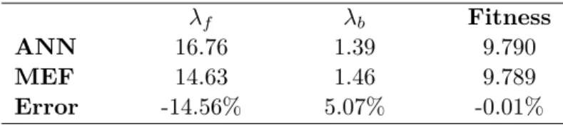
Table 6 Differences between ANN and FEM – Example 1.

λf λb Fitness

ANN _16.76 _1.39 _9.790

MEF _14.63 _1.46 _9.789

Error _-14.56% _5.07% _-0.01%

To verify the optimization quality, the design obtained with GA-ANN is compared to the design found using GA-FEM. This last design and parameters values are shown in Table 7.

Table 7 Results using GA-FEM – Example 1. Results

Laminate [_±45ge4 ,±45

ke_,₉₀ke 4 ]_S

λf 14.07

λb 1.54

W 27.34 N

C 46.93 uc/N

Fitness 9.789

GA Generations 146

Time 264.73 hours.

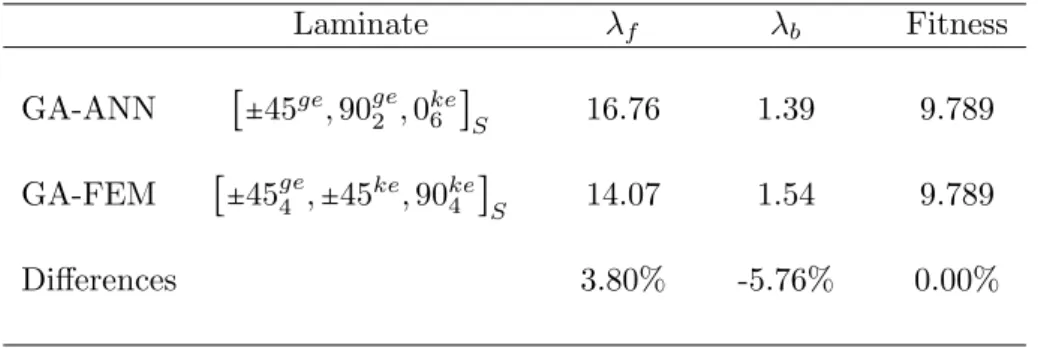
Differences between the designs obtained with GA-FEM and GA-ANN are shown in Table 8. These results show that the design obtained with the GA-ANN is a near optimum design.

(9)

Table 8 Differences between optimum designs – Example 1.

Laminate λf λb Fitness

GA-ANN [±45ge,90ge2 ,0 ke

6 ]_S 16.76 1.39 9.789

GA-FEM [±45ge4 ,±45

ke_,₉₀ke

4 ]_S 14.07 1.54 9.789

Differences 3.80% -5.76% 0.00%

Table 9 Processing time comparison (in hours) – Example 1.

GA-ANN GA-FEM

Training set generation 112.74

-Neural networks training 0.11

-GA execution 0.001 264.73

Total time 112.851 264.73

4.2 Stiffness maximization of a composite laminated shell with geometrically nonlinear behavior

This optimization problem aims to maximize the stiffness of a composite shallow shell under pressure load. Figure 3 shows the shell with its boundary and load conditions. The mesh has 800 elements. The nonlinear analysis is made using the GDCM method [12], with a load increment parameter λi = 0.05. The fitness function is defined in Eq. 3, where N Ccrit is the critical load level(when curve load - displacement reaches its first limit point), Umax is the maximum displacement, which is taken at the end of incremental load process or when material failure is observed, N Cmax is the maximum load level without material failure and Vnlc is a penalization for designs having more than 4 plies with same fiber orientation.

(10)

F IT N ESS =((N Ccrit)⋅(N C

2 max) (Umax)⋅(Vnlc+1) )

(3)

In the example glass-epoxy is used and the material properties are shown in Table 10.

Table 10 Properties of Glass-epoxy – Example 2.

Properties Values Properties Values

E1 39.0 GPa F1t 1080.0 MPa

E2 8.6 GPa F1c 620.0 MPa

G12 3.8 GPa F2t 39.0 MPa

ν12 0.28 F2c 128.0 MPa

ρ 20.6 KN/m3

F6 89.0 MPa

The genetic alphabet shown in Table 11 is used. In this example only the orientation of reinforcement fibers are the design variables, while the material, thickness and number of layers are fixed. The laminated has 28 plies (with thickness t=0.45mmfor each ply), the symmetry condition is imposed, each gene control 2 plies and the chromosome has 7 genes to control the laminate. Due to the long codification, for the crossover is used a double break point. The size of the design space (SDS) is 2187.

Table 11 Genetic codification alphabet – Example 2. Genes of the angles

code angle 1 2 plies a 0o 2 2 plies a ±45o

3 2 plies a 90o

The GA parameters used here are P =18,Ne =3,pma=5%, pmm0%,pgs=80%,ppa=0%, ppd=0%, NLG=108, NSD =36 with the same meaning as in the previous example.

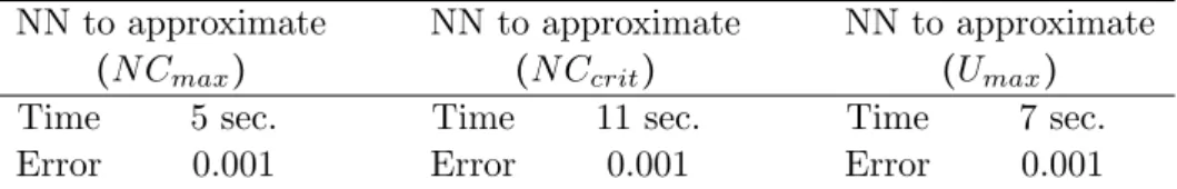
In this example, three neural networks are used to approximate each one of the parameters involved in the objective function (N Cmax, N Ccrit and Umax); each ANN for the trained parameters, errors and processing time are show in Table 12. The architecture adopted is 7:15:15:1. The training set has 226 designs and the time spent to generate this training set was 117.31 minutes.

Table 12 Neural Networks training time and errors – Example 2.

NN to approximate NN to approximate NN to approximate (N Cmax) (N Ccrit) (Umax)

Time 5 sec. Time 11 sec. Time 7 sec.

Error 0.001 Error 0.001 Error 0.001

(11)

Table 13 Results using GA-ANN – Example 2. Results

Laminate [904,±45,(902,02)2]S

(N Cmax) 0.989

(N Ccrit) 0.637

(Umax) 26.6×10−3m

Fitness 23.42

GA Generations 47

Time 0.01 min.

To evaluate the quality of the approximation using neural networks, the parameter values are compared to the parameter values for the same design using FEM without ANN. These differences are shown in Table 14.

Table 14 Differences between ANN and FEM – Example 2.

(N Cmax) (N Ccrit) (Umax) Fitness

ANN _0.989 _0.637 ₂₆.6×10−3m 23.42

FEM _1.000 _0.495 ₂₇_.₄_×₁₀−3

m 18.03

Error _1.10% _-28.62% _3.18% _-29.94%

Result and processing time used in the optimization process using GA-FEM is show in Table 15.

Table 15 Results using GA-FEM – Example 2. Results

Laminate [(904,±45)2,902]S

(N Cmax) 1.000

(N Ccrit) 0.560

(Umax) 27.2×10−3m

Fitness 20.60

GA Generations 40

Time 239.72 min.

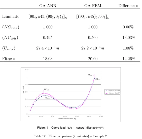
To verify the quality of the optimization process using GA-ANN, parameter values for both designs, obtained with ANN and FEM, are compared in Table 16. A graphical comparison of both designs is shown in Fig. 4, whereN Ccrit and Umax are indicated.

Processing time comparison, using GA-ANN and GA-FEM, is shown in Table 17.

(12)

Table 16 Differences of optimum designs obtained by GA-ANN and GA-FEM – Example 2.

GA-ANN GA-FEM Differences

Laminate [904,_±45,(902,02)2]S [(904,_±45)2,902]S

(N Cmax) 1.000 1.000 0.00%

(N Ccrit) 0.495 0.560 -13.03%

(Umax) 27.4×10− 3

m 27.2×10−3m 1.08%

Fitness 18.03 20.60 -14.26%

Figure 4 Curve load level – central displacement. Table 17 Time comparison (in minutes) – Example 2.

GA-ANN GA-MEF

-Neural Network training 0.65

Total time 117.97 239.72

4.3 Natural frequency maximization of a laminated plate

(13)

used to build this plate, and the material properties are given in Table 18.

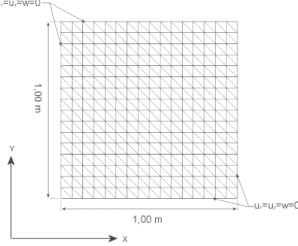
Figure 5 Composite laminated plate with its boundary conditions and the FE mesh.

Table 18 Properties of Graphite-epoxy.

Properties Values Properties Values

E1 181 GPa F1t 1500.0 MPa

E2 10.3 GPa F1c 1500.0 MPa

G12 7.17 GPa F2t 40.0 MPa

ν12 0.28 F2c 246.0 MPa

ρ 15.7 KN/m3

F6 68.0 MPa

The genetic alphabet used in this example is shown in Table 19. The chromosome length is 8. Double break point is used in the crossover operation. The size of the design space (SDS) is 6561.

Table 19 Genetic codification alphabet – Example 3. Angle genes

code angle 1 1 ply a 0o 2 1 ply a 45o 3 1 ply a 90o

The GA parameters used here are P =30,Ne =3,pma=5%, pmm0%,pgs=80%,ppa=0%, ppd=0%, NLG=200, NSD =100, with the same meaning as in the first example.

(14)

Table 20 Neural Network training time and error for Example 3. Neural network to approximateω

Time 1.25 min.

Error 0.01

Table 21 Result using GA-ANN – Example 3. Result

Laminate [90,45,03,90,452]S

ω 6.24 rad/s.

Generations 182

Time 0.03 min.

The design obtained here, as well as ω, are shown in Table 21

The difference of ω, obtained using ANN and FEM, is shown in Table 22.

Table 22 Difference between ANN and FEM – Example 3. ω

ANN _6.24

FEM _6.27

Error _0.48%

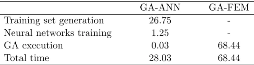
Making a GA-FEM optimization, the same design is found. A comparison of the processing time required for each method is shown in Table 23.

Table 23 Processing time comparison (in minutes) – Example 3.

GA-ANN GA-FEM

-Neural networks training 1.25

Total time 28.03 68.44

In this example the processing time saved is 59%. The optimization quality using ANN is high. This occurs because the function that has to be replaced by the neural network is very simple.

5 FINAL REMARKS

Some important remarks can be outlined from the examples, such as following:

(15)

GA-FEM. This is particularly true when Finite Elements Analyses are applied for structures requiring refined meshes and for cases where the structure has a nonlinear behavior.

• The optimum design is very little affected if well trained ANNs are used substituting

complete Finite Element Analyses, or, in other words, accuracy of ANNs can be improved with a longer and more elitist training set and increasing the number of GA application to generate samples of the training set.

• In cases where the cost function is simple, final design using GA-ANN will be very similar

to that obtained using GA-FEM.

In future works other kind of ANNs, such as ANN with Radial Basis, (substituting Mul-tilayer Perceptrons) will be tested. These tools (GAs and ANNs) may be employed also in Reliability Based Optimization Problems.

References

[1] Felipe Schaedler Almeida. Laminated composite material structures optimization with genetic algorithms. Master’s thesis, PPGEC/UFRGS, Porto Alegre, Rio Grande do Sul, Brazil, 2006. [in Portuguese].

[2] F.S. Almeida and A.M. Awruch. Design optimization of composite laminated structures using genetic algorithms and finite element analysis. Composite Structures, 88(3):443 – 454, 2009.

[3] Klaus-Jrgen Bathe and Lee-Wing Ho. A simple and effective element for analysis of general shell structures. Com-puters & Structures, 13(5-6):673 – 681, 1981.

[4] Isaac M. Daniel and Ori Ishai. Engineering Mechanics of Composite Materials. Oxford Press, 1994.

[5] David E. Goldberg. Genetic Algorithms in Search, Optimization, and Machine Learning. Addison-Wesley Profes-sional, January 1989.

[6] Herbert Martins Gomes and Armando Miguel Awruch. Comparison of response surface and neural network with other methods for structural reliability analysis.Structural Safety, 26(1):49 – 67, 2004.

[7] Simon Haykin. Neural Networks: A Comprehensive Foundation (2nd Edition). Prentice Hall, July 1998.

[8] Z. Luo and S. G. Hutton. Formulation of a three-node traveling triangular plate element subjected to gyroscopic and in-plane forces.Computers & Structures, 80(26):1935 – 1944, 2002.

[9] A. Muc and W. Gurba. Genetic algorithms and finite element analysis in optimization of composite structures.

Composite Structures, 54(2-3):275 – 281, 2001.

[10] G. Narayana Naik, S. Gopalakrishnan, and Ranjan Ganguli. Design optimization of composites using genetic algo-rithms and failure mechanism based failure criterion. Composite Structures, 83(4):354 – 367, 2008.

[11] Grant A. E. Soremekun. Genetic algorithms for composite laminate design and optimization. Master’s thesis, Department of Mechanical Engineering, Virginia Polytechnic Institute, Blacksburgh, Virginia, February 5 1997.