CONTRIBUTION OF AGRONOMIC TRAITS FOR SUGAR YIELD IN SWEET SORGHUM GENOTYPES

(1)

Versão impressa ISSN 1676-689X / Versão on line ISSN 1980-6477 http://www.abms.org.br

http://dx.doi.org/10.18512/1980-6477/rbms.v16n2p232-239

CONTRIBUTION OF AGRONOMIC TRAITS FOR SUGAR YIELD IN SWEET SORGHUM GENOTYPES

GESSI CECCON¹, PAULO EDUARDO TEODORO² and ADRIANO DOS SANTOS3

¹Embrapa Agropecuária Oeste, gessi.ceccon@embrapa.br; ²Universidade Federal de Viçosa, eduteodoro@hotmail.com;

³Universidade Estadual do Norte Fluminense Darcy Ribeiro, adriano_agro84@yahoo.com.br;

Revista Brasileira de Milho e Sorgo, v.16, n.2, p. 232-239, 2017

ABSTRACT - Currently, cultivation of sweet sorghum has increasing in traditional areas with new technologies in the sugar-ethanol industry. The aim of this study was to identify the agronomic traits that can be used for indirect selection of genotypes with higher sugar yield. The work was conducted in the 2014/2015 season, at Embrapa Agropecuária Oeste, in Dourados, MS. A total of 25 genotypes was evaluated in a randomized block design with three replications. The agronomic traits evaluated were: plant height, fresh mass, percentage of stems, leaves and panicles, dry mass, Brix, yield of juice and sugar. The F-test was used to check for genetic variability among genotypes. Phenotypic correlations among these traits were estimated, which are deployed through the path analysis in direct and indirect effects, considering the yield sugar as the primary dependent variable. The results showed that 92% of the variation in sugar yield was explained by the explanatory variables, value appropriate to explore the gains with indirect selection in sweet sorghum. The indirect selection based on Brix is the most effective way to obtain genetic progress in the sugar yield in sorghum genotypes.

Keywords: path analysis, correlations, direct and indirect effects, Sorghum bicolor.

CONTRIBUIÇÃO DE CARACTERES AGRONÔMICOS PARA A PRODUTIVIDADE DE AÇÚCAR EM GENÓTIPOS DE SORGO SACARINO

RESUMO - Atualmente, o sorgo sacarino tem apresentado grande expansão de cultivo em zonas tradicionais com o uso de novas tecnologias do setor sucroalcooleiro. O objetivo deste trabalho foi identificar quais caracteres agronômicos podem ser utilizados para seleção indireta de genótipos com maior produtividade de açúcar. O trabalho foi realizado na safra 2014/2015 na área experimental da Embrapa Agropecuária Oeste, em Dourados, MS. Foram avaliados 25 genótipos em delineamento experimental foi em blocos ao acaso com três repetições. Foram avaliados os seguintes caracteres agronômicos: altura de plantas, massa verde, porcentagem de colmo, de folhas, e panículas, massa seca, Brix, produtividade de caldo e açúcar. Foi aplicado o teste F para verificar a existência de variabilidade genética entre os genótipos. As correlações fenotípicas entre estes caracteres foram estimadas, sendo estas desdobradas, por meio da análise de trilha, em efeitos diretos e indiretos, considerando o caráter produtividade de açúcar como a variável dependente principal. Observou-se que 92% da variação na produtividade de açúcar foi explicada pelas variáveis explicativas, valor adequado para explorar os ganhos com a seleção indireta em sorgo sacarino. A seleção indireta com base no caráter Brix é o modo mais eficaz para se obter progresso genético na produtividade de açúcar de genótipos de sorgo sacarino.

(2)

Revista Brasileira de Milho e Sorgo, v.16, n.2, p. 232-239, 2017

Versão impressa ISSN 1676-689X / Versão on line ISSN 1980-6477 - http://www.abms.org.br

Contribution of agronomic traits for sugar yield in... 233

A great expansion of sweet sorghum (Sorghum bicolor L. Moench) cultivation has been currently observed in traditional, areas, as new technologies of the sugar and ethanol industry. This crop has stems with broth similar to sugarcane, rich in fermentable sugars and can be used to produce ethanol or sugar in the same facility used by sugarcane. It is an short cycle species (four months), with high productivity of

green biomass (60 to 80 Mg ha-1_{), high ethanol yields}

(3,000 to 6,000 l ha-1_{), TRS (total recoverable sugar)}

ranging from 4.8 to 7.6 Mg ha-1_{, and the bagasse can be}

used as an energy source (Pereira Filho et al., 2013). In this sense, one of the main aims of genetic breeding programs of sweet sorghum is selecting genotypes with increased productivity of sugar and/or ethanol. Thus, the, knowledge of correlations among agronomic traits is essential since can positively or negatively affect the genetic progress through indirect selection. In this case, the selection for a principal trait, characterized by its low heritability and/or measurement difficulties, it is practiced based on other(s) trait(s) with moderate to high heritability correlated to it, allowing the breeder to achieve more quick progress compared to the use of direct selection (Lynch & Walsh, 1998).

Cruz et al. (2014) emphasize that despite its importance, the correlations do not identify the cause and effect relation among the traits. In this sense, path analysis proposed by Wright (1921) allows better understanding the association between agronomic traits through the unfolding of the correlation coefficients into their direct and indirect effects on a principal trait, using regression equations of standardized variables (Corrar et al., 2007). For the sweet sorghum crop, there are few studies regarding the association

among agronomic traits (Sandeep et al., 2011; Rani

& Umakanth, 2012). Thus, the aim of this study was

to identify the agronomic traits that can be used for indirect selection of genotypes with high sugar content.

Material and Methods

The trial was conduct in the 2014/2015 season at the experimental area of Embrapa Agropecuária Oeste, in Dourados, MS (22°17’S,54°48›W and 380 m altitude). The soil of the experimental area was identified as Oxisol dystroferric clay texture. The climate is Cwa according to Köppen classification, with hot summers and dry winters.

A randomized block design was used with three replications, assessing 25 genotypes of sweet sorghum (BRS 506, BRS 508, BRS 509, BRS 511, CMSXS5003, CMSXS5004, CMSXS5006, CMSXS5007, CMSXS5008, CMSXS5009, CMSXS5010, CMSXS629, CMSXS630, CMSXS639, CMSXS643, CMSXS644, CMSXS646, CMSXS647, CMSXS648, CV 198, CV 568, Sugargraz, V82391, V82392 and V82393) from the breeding program of Embrapa Milho e Sorgo. The plots comprised four rows of five meters, spaced 0.50 m apart.

Seeds were sown in November 6, 2014, in no tillage system with emergence after seven days. Fertilization consisted of 200 kg ha-1_{(08-16-16) at}

sowing, more one topdressing with 50 kg ha-1_{of N.}

The weed control was performed with pre-sowing

desiccation with 1.44 L ha-1_{of glyphosate and one}

application of atrazine 1.2 kg ha-1_{20-25 days after}

emergence. Control of insect pests was carried out

by applying the insecticide Tiametoxam+

Lambda-Cialotrina (Engeo-pleno®₎_at_{0.005 L ha}-1_{.on the}

fifteenth day after emergence of maize.

At harvest, the following agronomic traits were evaluated: plant height (PH, m); fresh mass (FM, kg

(3)

Versão impressa ISSN 1676-689X / Versão on line ISSN 1980-6477 - http://www.abms.org.br Ceccon et al.

234

(PL, %), percentage of panicles (PP, %), dry mass

(DM, kg ha-1_{), broth yield (BY, l ha}-1_{), Brix (ºbrix) and}

sugar yield (SY, kg ha-1_{). PH was measured in five}

plants per plot. FM was assessed by harvesting and weighing the central rows of each plot. A subsample of five plants was removed for separation of stems, leaves and panicles to determine the PS, PL and PP. Subsequently, this sample was dried in an oven at 65°C for 72 h to determine DM. The BY was calculated by the difference between the FM and DM. Brix was evaluated using Portable Digital Refractometer with range 0-45% of Brix.

In order to verify the existence of variability between genotypes, data were submitted to analysis of variance by F test, considering the effects of genotypes as fixed and others as random. The following genetic parameters were determined: environmental variance -

3 the agronomic traits that can be used for indirect selection of genotypes with high sugar content.

The trial was conduct in the 2014/2015 season at the experimental area of Embrapa Agropecuária Oeste, in Dourados, MS (22°17'S,54°48'W and 380 m altitude). The soil of the experimental area was identified as Oxisoldystroferric clay texture. The climate is Cwa according to Köppen classification, with hot summers and dry winters.

Seeds were sown in November 6, 2014, in no tillage system with emergence after seven days. Fertilization consisted of 200 kg ha-1_{(08-16-16) at sowing, more one topdressing} with 50 kg ha-1_{of N. The weed control was performed with pre-sowing desiccation with 1.44} L ha-1_{of glyphosate and one application of atrazine 1.2 kg ha}-1_{20-25 days after emergence.} Control of insect pests was carried out by applying the insecticide Tiametoxam+ Lambda-Cialotrina (Engeo-pleno®_{) at 0.005 L ha}-1_{.on the fifteenth day after emergence of maize.}

At harvest, the following agronomic traits were evaluated: plant height (PH, m); fresh mass (FM, kg ha-1_{); percentage of stem (PS, %), percentage of leaves (PL, %), percentage of} panicles (PP, %), dry mass (DM, kg ha-1_{), broth yield (BY, l ha}-1_{), Brix (ºbrix) and sugar yield} (SY, kg ha-1_{). PH was measured in five plants per plot. FM was assessed by harvesting and} weighing the central rows of each plot. A subsample of five plants was removed for separation of stems, leaves and panicles to determine the PS, PL and PP. Subsequently, this sample was dried in an oven at 65°C for 72 h to determine DM. The BY was calculated by the difference between the FM and DM. Brix was evaluated using Portable Digital Refractometer with range 0-45% of Brix.

k MS σˆ2 r E , phenotypic variance - _k MS σˆ2 g

P and genotypic variance - _k MS -MS σˆ2 g r G ; , phenotypic variance - 3 the agronomic traits that can be used for indirect selection of genotypes with high sugar content.

The trial was conduct in the 2014/2015 season at the experimental area of Embrapa Agropecuária Oeste, in Dourados, MS (22°17'S,54°48'W and 380 m altitude). The soil of the experimental area was identified as Oxisoldystroferric clay texture. The climate is Cwa according to Köppen classification, with hot summers and dry winters.

P and genotypic variance - _k MS -MS σˆ2 g r

G ;

and genotypic variance -

3 the agronomic traits that can be used for indirect selection of genotypes with high sugar content.

The trial was conduct in the 2014/2015 season at the experimental area of Embrapa Agropecuária Oeste, in Dourados, MS (22°17'S,54°48'W and 380 m altitude). The soil of the experimental area was identified as Oxisol dystroferric clay texture. The climate is Cwa according to Köppen classification, with hot summers and dry winters.

P and genotypic variance - _k MS -MS σˆ2 g r G ; coefficient ; of experimental variation - 4

coefficient of experimental variation - 100 m MS CV e e _      

 and coefficient of genotypic

variation - 100 m σ CV 2G g       

 ; genotypic coefficient of determination -

F G 2 σˆ σˆ R  ; quotient b - e g CV CV b  ; phenotypic correlations - ₂ Py 2 ´Px F(xy) σ σ COV r  

P , wherein MSr is the mean square of

the residue; MSg is the mean square of the genotype; k is the number of repetitions; m is the

overall mean of the trial; COVF(xy) is the covariance between traits X and Y; 2 Fx σ and 2

Fy σ are the variances between traits X and Y, respectively. The significance of the phenotypic correlation was verified by the t-test with n-2 degrees of freedom.

The rF were deployed through the path analysis into direct and indirect effects,

considering the following model: Y = p1X1 + p2X2 + ... + pnXn + pεu, wherein Y is the

principal dependent variable (PD); X1, X2, ..., xn: are the independent explanatory variables;

p1, p2, ..., pn: are the path analysis coefficients. The coefficient of determination was

calculated by the expression R2_{= p}_1y2_{+ p}_2y2_{+ ... 2p}_2y_p_2n_r_2n_{(Wright, 1921).}

Degree of multicollinearity of X'X matrix was determined based on the condition number (CN), which is the ratio between the largest and the smallest eigenvalue of the matrix (Montgomery & Peck, 2001). If CN<100, multicollinearity is called weak and is not a problem for analysis; if 100≤CN≤1,000, multicollinearity is considered moderate to strong; and if CN>1,000 the degree of multicollinearity is determined as severe. All statistical analyzes were performed using the GENES software (Cruz, 2013).

Results and Discussion

Significant differences (p<0.01) among genotypes were observed for all traits (Table 1), allowing to infer the existence of genetic variability of this population. Quantifying the genetic variability of the studied population is a determining factor in a breeding program, since allows knowing the genetic structure of the population. Similar results were obtained in other studies with the sweet sorghum crop (Albuquerque et al., 2012; May et al., 2012; Pereira Filho et al., 2013). The variance of the genotypic effects (2

g

σˆ) was higher than the variance of the environmental effects ( 2

e

σˆ), for all traits evaluated. As the genetic variance

and coefficient of genotypic variation -

4

Significant differences (p<0.01) among genotypes were observed for all traits (Table 1), allowing to infer the existence of genetic variability of this population. Quantifying the genetic variability of the studied population is a determining factor in a breeding program, since allows knowing the genetic structure of the population. Similar results were obtained in other studies with the sweet sorghum crop (Albuquerque et al., 2012; May et al., 2012; Pereira Filho et al., 2013). The variance of the genotypic effects ( 2

g

e

; genotypic coefficient of determination

-4

g

e

; quotient b -

4

g

e

; phenotypic correlations -

4

coefficient of experimental variation - 100 m MS CV e e _     

F G 2 σˆ σˆ R  ; quotient b - e g CV CV b  ; phenotypic correlations - 2 Py 2 ´Px F(xy) σ σ COV r  

overall mean of the trial; COVF(xy) is the covariance between traits X and Y; σ2Fx and σ2Fy are

the variances between traits X and Y, respectively. The significance of the phenotypic correlation was verified by the t-test with n-2 degrees of freedom.

calculated by the expression R2_{= p}

1y2 + p2y2 + ... 2p2yp2nr2n (Wright, 1921).

g

e

, wherein MSr is the

mean square of the residue; MSg is the mean square

of the genotype; k is the number of repetitions; m is the overall mean of the trial;

4

coefficient of experimental variation - 100

m MS CV e e _      

variation - 100 m σ CV 2G g _      

F G 2 σˆ σˆ R  ; quotient b - e g CV CV b  ; phenotypic correlations - 2 Py 2 ´Px F(xy) σ σ COV r  

overall mean of the trial; COVF(xy) is the covariance between traits X and Y;

2 Fx

σ and 2

Fy

σ are

the variances between traits X and Y, respectively. The significance of the phenotypic correlation was verified by the t-test with n-2 degrees of freedom.

calculated by the expression R2_{= p}

Significant differences (p<0.01) among genotypes were observed for all traits (Table 1), allowing to infer the existence of genetic variability of this population. Quantifying the genetic variability of the studied population is a determining factor in a breeding program, since allows knowing the genetic structure of the population. Similar results were obtained in other studies with the sweet sorghum crop (Albuquerque et al., 2012; May et al., 2012;

Pereira Filho et al., 2013). The variance of the genotypic effects ( 2

g

σˆ) was higher than the

variance of the environmental effects ( 2

e

σˆ ), for all traits evaluated. As the genetic variance

is the covariance between traits X and Y;

4

 ; genotypic coefficient of determination - F G 2 σˆ σˆ R  ; quotient b - e g CV CV b  ; phenotypic correlations - ₂ Py 2 ´Px F(xy) σ σ COV r  

P , wherein MSr is the mean square of the residue; MSg is the mean square of the genotype; k is the number of repetitions; m is the overall mean of the trial; COVF(xy) is the covariance between traits X and Y;

2 Fx

σ and 2 Fy

σ are the variances between traits X and Y, respectively. The significance of the phenotypic correlation was verified by the t-test with n-2 degrees of freedom.

The rF were deployed through the path analysis into direct and indirect effects, considering the following model: Y = p1X1 + p2X2 + ... + pnXn + pεu, wherein Y is the principal dependent variable (PD); X1, X2, ..., xn: are the independent explanatory variables; p1, p2, ..., pn: are the path analysis coefficients. The coefficient of determination was calculated by the expression R2_{= p}

g

e

and

4

 ; genotypic coefficient of determination - F G 2 σˆ σˆ R  ; quotient b - e g CV CV b  ; phenotypic correlations - ₂ Py 2 ´Px F(xy) σ σ COV r  

P , wherein MSr is the mean square of the residue; MSg is the mean square of the genotype; k is the number of repetitions; m is the overall mean of the trial; COVF(xy) is the covariance between traits X and Y;

2 Fx

σ and 2 Fy

σ are the variances between traits X and Y, respectively. The significance of the phenotypic correlation was verified by the t-test with n-2 degrees of freedom.

The rF were deployed through the path analysis into direct and indirect effects, considering the following model: Y = p1X1 + p2X2 + ... + pnXn + pεu, wherein Y is the principal dependent variable (PD); X1, X2, ..., xn: are the independent explanatory variables; p1, p2, ..., pn: are the path analysis coefficients. The coefficient of determination was calculated by the expression R2_{= p}

g

e

are the variances between traits X and Y, respectively. The significance of the phenotypic correlation was verified by the t-test with n-2 degrees of freedom.

The rF were deployed through the path analysis

into direct and indirect effects, considering the

following model: Y = p₁X₁ + p₂X₂ + ... + p_nX_n + p_εu,

wherein Y is the principal dependent variable (PD); X₁,

X₂, ..., xn: are the independent explanatory variables;

p₁, p₂, ..., p_n: are the path analysis coefficients. The

coefficient of determination was calculated by the

expression R2_{= p}

1y2 + p2y2 + ... 2p2yp2nr2n (Wright,

1921).

Degree of multicollinearity of X’X matrix was determined based on the condition number (CN), which is the ratio between the largest and the smallest eigenvalue of the matrix (Montgomery & Peck, 2001). If CN<100, multicollinearity is called weak and is not a problem for analysis; if 100≤CN≤1,000, multicollinearity is considered moderate to strong; and if CN>1,000 the degree of multicollinearity is determined as severe. All statistical analyzes were performed using the GENES software (Cruz, 2013).

Significant differences (p<0.01) among genotypes were observed for all traits (Table 1), allowing to infer the existence of genetic variability of this population. Quantifying the genetic variability of the studied population is a determining factor in a breeding program, since allows knowing the genetic structure of the population. Similar results were obtained in other studies with the sweet sorghum crop (Albuquerque et al., 2012; May et al., 2012; Pereira Filho et al., 2013). The variance of the genotypic effects (

4 coefficient of experimental variation -

100 m

MS

CV

e e

_

















and coefficient of genotypic

variation -

100 m

σ

CV

g 2G

_

















; genotypic coefficient of determination -

F G 2

σˆ

R 

; quotient

b -

e g

CV

b 

; phenotypic correlations -

₂ Py 2 ´Px F(xy)

σ

COV

r





P

, wherein

MS

r

is the mean square of

the residue;

MS

g

is the mean square of the genotype; k is the number of repetitions; m is the

overall mean of the trial;

COV

F(xy)

is the covariance between traits X and Y;

2 Fx

σ

and

2

Fy

σ

are

the variances between traits X and Y, respectively. The significance of the phenotypic

correlation was verified by the t-test with n-2 degrees of freedom.

The

r

F

were deployed through the path analysis into direct and indirect effects,

considering the following model: Y = p

1

X

1

+ p

2

X

2

+ ... + p

n

X

n

+ p

ε

u, wherein Y is the

principal dependent variable (PD); X

1

, X

2

, ..., xn: are the independent explanatory variables;

p

1

, p

2

, ..., p

n

: are the path analysis coefficients. The coefficient of determination was

calculated by the expression R

2

_{= p}

1y2

+ p

2y2

+ ... 2p

2y

p

2n

r

2n

(Wright, 1921).

Degree of multicollinearity of X'X matrix was determined based on the condition

number (CN), which is the ratio between the largest and the smallest eigenvalue of the matrix

(Montgomery & Peck, 2001). If CN<100, multicollinearity is called weak and is not a

problem for analysis; if 100≤CN≤1,000, multicollinearity is considered moderate to strong;

and if CN>1,000 the degree of multicollinearity is determined as severe. All statistical

analyzes were performed using the GENES software (Cruz, 2013).

Results and Discussion

Significant differences (p<0.01) among genotypes were observed for all traits (Table

1), allowing to infer the existence of genetic variability of this population. Quantifying the

genetic variability of the studied population is a determining factor in a breeding program,

since allows knowing the genetic structure of the population. Similar results were obtained in

other studies with the sweet sorghum crop (Albuquerque et al., 2012; May et al., 2012;

Pereira Filho et al., 2013). The variance of the genotypic effects (

2

g

σˆ

) was higher than the

variance of the environmental effects (

2

e

σˆ

), for all traits evaluated. As the genetic variance

) was higher than the variance of the environmental effects (

4 coefficient of experimental variation -

100 m

MS

CV

e e

_

















and coefficient of genotypic

variation -

100 m

σ

CV

g 2G

_

















; genotypic coefficient of determination -

F G 2

σˆ

R 

; quotient

b -

e g

CV

b 

; phenotypic correlations -

2 Py 2 ´Px F(xy)

σ

COV

r





P

, wherein

MS

r

is the mean square of

the residue;

MS

g

is the mean square of the genotype; k is the number of repetitions; m is the

overall mean of the trial;

COV

F(xy)

is the covariance between traits X and Y;

2 Fx

σ

and

2

Fy

σ

are

the variances between traits X and Y, respectively. The significance of the phenotypic

correlation was verified by the t-test with n-2 degrees of freedom.

The

r

F

were deployed through the path analysis into direct and indirect effects,

considering the following model: Y = p

1

X

1

+ p

2

X

2

+ ... + p

n

X

n

+ p

ε

u, wherein Y is the

principal dependent variable (PD); X

1

, X

2

, ..., xn: are the independent explanatory variables;

p

1

, p

2

, ..., p

n

: are the path analysis coefficients. The coefficient of determination was

calculated by the expression R

2

_{= p}

1y2

+ p

2y2

+ ... 2p

2y

p

2n

r

2n

(Wright, 1921).

Degree of multicollinearity of X'X matrix was determined based on the condition

number (CN), which is the ratio between the largest and the smallest eigenvalue of the matrix

(Montgomery & Peck, 2001). If CN<100, multicollinearity is called weak and is not a

problem for analysis; if 100≤CN≤1,000, multicollinearity is considered moderate to strong;

and if CN>1,000 the degree of multicollinearity is determined as severe. All statistical

analyzes were performed using the GENES software (Cruz, 2013).

Results and Discussion

Significant differences (p<0.01) among genotypes were observed for all traits (Table

1), allowing to infer the existence of genetic variability of this population. Quantifying the

genetic variability of the studied population is a determining factor in a breeding program,

since allows knowing the genetic structure of the population. Similar results were obtained in

other studies with the sweet sorghum crop (Albuquerque et al., 2012; May et al., 2012;

Pereira Filho et al., 2013). The variance of the genotypic effects (

2

g

σˆ

) was higher than the

variance of the environmental effects (

2

e

σˆ

), for all traits evaluated.

), for all traits evaluated. As the genetic variance

As the genetic variance component is caused by

genetic differences between individuals, so a high value of this component corroborates a wide genetic variability, indicating the possibility of obtaining gains with the selection (Cruz et al., 2014).

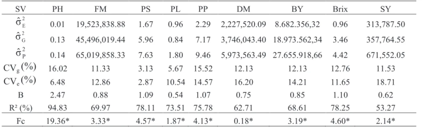
Coefficient of experimental variation (CV_e)

ranged from 2.87% (PS) to 18.71% (SY), similar to the values obtained in other studies on sweet sorghum (Albuquerque et al., 2012; May et al., 2012; Pereira Filho et al., 2013). According to Cruz et al. (2014),

(4)

Table 1. Genetic parameters and F values calculated (Fc) for the traits plant height (PH), fresh mass (FM),

percentage of stem (PS), percentage of leaves (PL), percentage of panicles (PP), dry mass (DM), broth yield (BY), Brix and sugar yield (SY), evaluated in 25 sweet sorghum genotypes.

*: significant at 1% probability by F-test; CVe= coefficient of variation;

5 component is caused by genetic differences between individuals, so a high value of this

component corroborates a wide genetic variability, indicating the possibility of obtaining

gains with the selection (Cruz et al., 2014).

Table 1. Genetic parameters and F values calculated (Fc) for the traits plant height (PH),

fresh mass (FM), percentage of stem (PS), percentage of leaves (PL), percentage of panicles

(PP), dry mass (DM), broth yield (BY), Brix and sugar yield (SY), evaluated in 25 sweet

sorghum genotypes.

σˆ

2P= phenotypic variance;

σ

2G= genotypic variance;

σ

2_E= environmental variance; R²= genotypic coefficient of determination; CVg= coefficient of genotypic variation, b= quotient b.

Coefficient of experimental variation (CV

e

) ranged from 2.87% (PS) to 18.71% (SY),

similar to the values obtained in other studies on sweet sorghum (Albuquerque et al., 2012;

May et al., 2012; Pereira Filho et al., 2013). According to Cruz et al. (2014), continuous

phenotypic traits with values less than 20% reflect excellent experimental accuracy. Under

another interpretation, coefficient of genetic variation (CV

g

) quantifies the magnitude of

genetic variation for selection and, therefore, higher values are desirable. However, to have a

real overview of the situation of each trait aimed at improving, it is necessary to analyze the

(CV

g

) together with CVe, by CV

g

/CVe ratio. In this context, the traits PH, PS, PP and Brix

showed values greater than unit, indicating a very favorable situation for selection (Resende

& Duarte, 2007).

Heritability is one of the parameters that most contributes for the breeder’s work

because it provides the proportion of genetic variance present in the total phenotypic variance.

Thus, it measures the reliability of phenotypic value as an indicator of reproductive value.

Heritability estimates above 75% is considered high, indicating to be a promising trait for

selection. Cruz et al. (2014) mention that when the statistical model considers the genotypes

as fixed effect, as in this study, heritability should be called of genotypic coefficient of

determination (R²). R² estimates above 75% were observed for the traits PH, PS PP and Brix

(Table 1), which together to the quotient b allow inferring that these traits are subject to

significant genetic gains into successive selection cycle.

There were positive and significant correlations between the traits PH x FM; PH, PP,

PH x BY, FM x DM, FM x BY, PS x SY, DM x BY, BY x YS and Brix x SY, and negative

= phenotypic variance;

5 component is caused by genetic differences between individuals, so a high value of this

component corroborates a wide genetic variability, indicating the possibility of obtaining

gains with the selection (Cruz et al., 2014).

Table 1. Genetic parameters and F values calculated (Fc) for the traits plant height (PH),

fresh mass (FM), percentage of stem (PS), percentage of leaves (PL), percentage of panicles

(PP), dry mass (DM), broth yield (BY), Brix and sugar yield (SY), evaluated in 25 sweet

sorghum genotypes.

σˆ

2P= phenotypic variance;

σ

2G= genotypic variance;

σ

Coefficient of experimental variation (CV

e

) ranged from 2.87% (PS) to 18.71% (SY),

similar to the values obtained in other studies on sweet sorghum (Albuquerque et al., 2012;

May et al., 2012; Pereira Filho et al., 2013). According to Cruz et al. (2014), continuous

phenotypic traits with values less than 20% reflect excellent experimental accuracy. Under

another interpretation, coefficient of genetic variation (CV

g

) quantifies the magnitude of

genetic variation for selection and, therefore, higher values are desirable. However, to have a

real overview of the situation of each trait aimed at improving, it is necessary to analyze the

(CV

g

) together with CVe, by CV

g

/CVe ratio. In this context, the traits PH, PS, PP and Brix

showed values greater than unit, indicating a very favorable situation for selection (Resende

& Duarte, 2007).

Heritability is one of the parameters that most contributes for the breeder’s work

because it provides the proportion of genetic variance present in the total phenotypic variance.

Thus, it measures the reliability of phenotypic value as an indicator of reproductive value.

Heritability estimates above 75% is considered high, indicating to be a promising trait for

selection. Cruz et al. (2014) mention that when the statistical model considers the genotypes

as fixed effect, as in this study, heritability should be called of genotypic coefficient of

determination (R²). R² estimates above 75% were observed for the traits PH, PS PP and Brix

(Table 1), which together to the quotient b allow inferring that these traits are subject to

significant genetic gains into successive selection cycle.

There were positive and significant correlations between the traits PH x FM; PH, PP,

PH x BY, FM x DM, FM x BY, PS x SY, DM x BY, BY x YS and Brix x SY, and negative

= genotypic variance;

5 component is caused by genetic differences between individuals, so a high value of this

component corroborates a wide genetic variability, indicating the possibility of obtaining

gains with the selection (Cruz et al., 2014).

Table 1. Genetic parameters and F values calculated (Fc) for the traits plant height (PH),

fresh mass (FM), percentage of stem (PS), percentage of leaves (PL), percentage of panicles

(PP), dry mass (DM), broth yield (BY), Brix and sugar yield (SY), evaluated in 25 sweet

sorghum genotypes.

σˆ

2_P= phenotypic variance;

σ

2_G= genotypic variance;

σ

Coefficient of experimental variation (CV

e

) ranged from 2.87% (PS) to 18.71% (SY),

similar to the values obtained in other studies on sweet sorghum (Albuquerque et al., 2012;

May et al., 2012; Pereira Filho et al., 2013). According to Cruz et al. (2014), continuous

phenotypic traits with values less than 20% reflect excellent experimental accuracy. Under

another interpretation, coefficient of genetic variation (CV

g

) quantifies the magnitude of

genetic variation for selection and, therefore, higher values are desirable. However, to have a

real overview of the situation of each trait aimed at improving, it is necessary to analyze the

(CV

g

) together with CVe, by CV

g

/CVe ratio. In this context, the traits PH, PS, PP and Brix

showed values greater than unit, indicating a very favorable situation for selection (Resende

& Duarte, 2007).

Heritability is one of the parameters that most contributes for the breeder’s work

because it provides the proportion of genetic variance present in the total phenotypic variance.

Thus, it measures the reliability of phenotypic value as an indicator of reproductive value.

Heritability estimates above 75% is considered high, indicating to be a promising trait for

selection. Cruz et al. (2014) mention that when the statistical model considers the genotypes

as fixed effect, as in this study, heritability should be called of genotypic coefficient of

determination (R²). R² estimates above 75% were observed for the traits PH, PS PP and Brix

(Table 1), which together to the quotient b allow inferring that these traits are subject to

significant genetic gains into successive selection cycle.

There were positive and significant correlations between the traits PH x FM; PH, PP,

PH x BY, FM x DM, FM x BY, PS x SY, DM x BY, BY x YS and Brix x SY, and negative

= environmental variance; R²= genotypic coefficient of determination; CVg= coefficient of genotypic variation, b= quotient b.

continuous phenotypic traits with values less than 20% reflect excellent experimental accuracy. Under another interpretation, coefficient of genetic variation

(CV_g) quantifies the magnitude of genetic variation for

selection and, therefore, higher values are desirable. However, to have a real overview of the situation of each trait aimed at improving, it is necessary to analyze

the (CV_g ) together with CVe, by CV_g/CVe ratio. In

this context, the traits PH, PS, PP and Brix showed

values greater than unit, indicating a very favorable situation for selection (Resende & Duarte, 2007).

Heritability is one of the parameters that most contributes for the breeder’s work because it provides the proportion of genetic variance present in the total phenotypic variance. Thus, it measures the reliability of phenotypic value as an indicator of reproductive value. Heritability estimates above 75% is considered high, indicating to be a promising trait for selection. Cruz et al. (2014) mention that when the statistical model considers the genotypes as fixed effect, as in this study, heritability should be called of genotypic coefficient of determination (R²). R² estimates above

75% were observed for the traits PH, PS PP and Brix (Table 1), which together to the quotient b allow inferring that these traits are subject to significant genetic gains into successive selection cycle.

There were positive and significant correlations between the traits PH x FM; PH, PP, PH x BY, FM x DM, FM x BY, PS x SY, DM x BY, BY x YS and Brix x SY, and negative and significant between PH x Brix and PS x PP (Table 2), similar to the noticed by Sandeep et al. (2011), Rani and Umakanth (2012) and Figueiredo et al. (2015). The main cause of phenotypic correlation between two traits is the pleiotropism, property by which a gene affects more than one trait simultaneously; and linkage disequilibrium, non-random association between alleles from different loci (Mode & Robinson, 1959). Correlation allows assessing the degree of association between two traits and the viability of the indirect selection, which in some cases can lead to more rapid progress than the desired trait selection (Cruz et al., 2014). However, the selection of a trait can lead to an undesirable selection of another. SV PH FM PS PL PP DM BY Brix SY 2 E

σˆ

_{0.01 19,523,838.88 1.67} _{0.96 2.29 2,227,520.09 8.682.356,32 0.96} _313,787.50 2 G

σˆ

_{0.13 45,496,019.44 5.96} _{0.84 7.17 3,746,043.40 18.973.562,34 3.46} _357,764.55 2 P

σˆ

_{0.14 65,019,858.33 7.63} _{1.80 9.46 5,973,563.49 27.655.918,66 4.42} _671,552.05 CVg

(%)

16.02 11.33 3.13 5.67 15.52 12.13 12.13 12.76 11.53 CVe

(%)

6.48 12.86 2.87 10.54 14.57 16.20 14.21 11.65 18.71 B 2.47 0.88 1.09 0.54 1.07 0.75 0.85 1.10 0.62 R² (%) 94.83 69.97 78.11 73.51 75.78 62.71 68.61 78.25 53.27 Fc 19.36* 3.33* 4.57* 1.87* 4.13* 0.18* 3.19* 4.60* 2.14*

(5)

236

Table 2. Phenotypic correlations between the traits plant height (PH), fresh mass (FM), percentage of stem

(PS), percentage of leaves (PL), percentage of panicles (PP), dry mass (DM), broth yield (BY), Brix and sugar yield (SY), evaluated in 25 sweet sorghum genotypes.

*: significant at 5% probability by t-test with n-2 degrees of freedom.

Thus, although important, coefficient of phenotypic correlation can produce misconceptions about the relation between two traits, and may not be a true measure of cause and effect. A high or low coefficient of correlation between two traits may be the result of the effect that a third trait or group of traits has on the pair, not giving the exact relative importance of the direct and indirect effects of these factors (Cruz et al., 2014). Therefore, the path analysis was performed, which investigates the relationship of cause and effect. Teodoro et al. (2014) pointed that this analysis provides a detailed knowledge on the effects of the traits involved, and justify the existence of positive and negative correlations, high and low magnitude, between the traits studied.

However, for obtaining the direct and indirect effects of path analysis, it is necessary that the X’X matrix be well conditioned. Under the presence of multicollinearity, the variances associated with the estimators of the path coefficients may to achieve excessively high values, making it unreliable. In addition, the parameter estimates can assume absurd values or no consistency with the studied biological phenomenon (Cruz et al., 2014). Matrix

of the estimates of phenotypic correlations presented strong multicollinearity (CN>100) based on criterion presented by Montgomery and Peck (2001).

It was already expected problem with multicollinearity, since in the analysis are involved biologically dependent traits. However, this result does not invalidate performing the path analysis because there are appropriate methodologies for studying the direct and indirect effects under multicollinearity (Carvalho, 1995; Coimbra et al., 2005). Thus, the methodology proposed by Carvalho (1995) was used in this study to estimate the direct and indirect effects, denominated path analysis in crest. This methodology consists of adding to the diagonal of the X’X matrix a k constant (0<k<1) which will correct CN to values lower than 100. The lowest k value (0.05) that provided weak multicolinearity (CN<100) was found graphically and allowed to use all traits evaluated in the path analysis.

In breeding, it is important to identify among the variables of high correlation with the basic variable those with the greatest direct effect favorable to the selecting towards, so that the response correlated by indirect selection be efficient. Thus, the traits FM, BY

Trait FM PS PL PP DM BY Brix SY PH 0.72* -0.39 -0.33 0.50* 0.70* 0.56* -0.58* 0.01 FM -0.16 -0.42 0.32 0.78* 0.94* -0.47 0.45 PS 0.00 -0.90* -0.39 0.14 0.44 0.50* PL -0.44 -0.26 -0.47 0.18 -0.26 PP 0.46 0.07 -0.48 -0.34 DM 0.56* -0,6 0.29 BY -0.41 0.55* Brix 0.53*

(6)

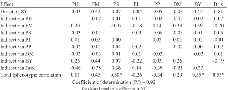
Table 3. Estimates of the direct and indirect effects of the traits plant height (PH), fresh mass (FM), percentage

of stem (PS), percentage of leaves (PL), percentage of panicles (PP), dry mass (DM), broth yield (BY), Brix and sugar yield (SY), evaluated in 25 sweet sorghum genotypes.

*: significant at 5% probability by t-test with n-2 degrees of freedom.

and Brix were the most important for indirect selection for increasing SY by presenting the greatest direct effects, indicating the presence of cause and effect (Table 3). FM and BY showed indirect and positive effects on each other and negatively affected the Brix. Thus, it is necessary special careful when using any of these traits for selecting sorghum genotypes with high SY, since the direct selection based on one of these traits can negatively affect others. Therefore, based on the genetic parameters initially evaluated (quotient b and R²), the use of Brix is recommend so that the breeder get quicker genetic progress on SY.

PS presented a positive and significant correlation (0.5) with the principal dependent variable, but null direct effect (0.07). This indicates that this correlation was caused by indirect effects, especially the trait Brix. According to Coimbra et al. (2005), when observing high and negative direct effects as well as low-magnitude indirect, indirect selection can

not to provide satisfactory gains. Thus, employment of simultaneous selection of traits is more appropriate (Cruz et al., 2014).

Coefficient of determination (Table 3) indicates that 92% of the dependent variable (SY) can be explained by the effect of the explanatory variables, which is higher than those reported by

Sandeep et al. (2011) and Rani and Umakanth

(2012). However, it should be considered that the SY is a complex inheritance trait (low R²), controlled by quantitative genes, being strongly affected by climatic and soil features. In this regard, the effect of the residual variable, although relatively low (0.27), suggests that indirect effects may have acted on SY. Thus, indirect selection does not always will provide gains on principal dependent variable, making the simultaneous selection also should be carefully considered as a way to achieving gains on the trait of

interest (Cruz et al., 2014). Thus, it is recommended

Effect PH FM PS PL PP DM BY Brix Direct on SY -0.03 0.42 0.07 -0.04 -0.05 -0.03 0.47 0.81 Indirect via PH -0.02 0.01 0.01 -0.02 -0.02 -0.02 0.02 Indirect via FM 0.30 -0.07 -0.18 0.14 0.33 0.39 -0.20 Indirect via PS -0.03 -0.01 0.00 -0.06 -0.03 0.01 0.03 Indirect via PL 0.01 0.02 0.00 0.02 0.01 0.02 -0.01 Indirect via PP -0.02 -0.01 0.04 0.02 -0.02 0.00 0.02 Indirect via DM -0.02 -0.03 0.01 0.01 -0.02 -0.02 0.01 Indirect via BY 0.26 0.44 0.07 -0.22 0.03 0.26 -0.19

Indirect via Brix -0.46 -0.38 0.36 0.14 -0.38 -0.21 -0.33

Total (phenotypic correlation) 0.01 0.45 0.50* -0.26 -0.34 0.29 0.55* 0.53*

Coefficient of determination (R²) = 0.92 Residual variable effect = 0.27

(7)

238

for future studies the development of a selection index with the traits FM, BY and Brix for identifying sweet sorghum genotypes with high SY.

Conclusion

Indirect selection based on Brix is the most efficient way to obtain genetic gain in sugar yield of sweet sorghum genotypes.

References

ALBUQUERQUE, C. J. B.; TARDIN, F. D.; PARRELA, R. A. C.; GUIMARÃES, A. S.; OLIVEIRA, R. M.; SILVA, K. M. J. Sorgo sacarino em diferentes arranjos de plantas e localidades de Minas Gerais, Brasil. Revista Brasileira

de Milho e Sorgo, Sete Lagoas, v. 11, n. 1, p. 69-85, 2012.

DOI: 10.18512/1980-6477/rbms.v11n1p69-85.

ALMODARES, A.; HADI, M. R. Production of bioethanol from sweet sorghum: a review. African Journal of

Agricultural Research, Nairobi, v. 4, n. 9, p. 772-780,

2009.

CARVALHO, S. P. Métodos alternativos de estimação

de coeficientes de trilha e índices de seleção, sob multicolinearidade. Viçosa, MG: Universidade Federal

de Viçosa, 1995. 163 p.

COIMBRA, J. L. M.; BENIN, G.; VIEIRA, E. A.; OLIVEIRA, A. C.; CARVALHO, F. I. F.; GUIDOLIN, A. F.; SOARES, A. P. Conseqüências da multicolinearidade sobre a análise de trilha em canola. Ciência Rural, Santa Maria, v. 35, n. 2, p. 347-352, 2005.

DOI: 10.1590/S0103-84782005000200015.

CORRAR, L. J.; PAULO, E.; DIAS FILHO, J. M. Análise

multivariada. Atlas: FIPECAFI, 2007. 542 p.

CRUZ, C. D. GENES: a software package for analysis in experimental statistics and quantitative genetics. Acta

Scientiarum. Agronomy, Maringá, v. 35, n. 3, p. 271-276,

2013. DOI: 10.4025/actasciagron.v35i3.21251.

CRUZ C. D.; CARNEIRO, P. C.; REGAZZI A. J. Modelos

biométricos aplicados ao melhoramento genético.

Viçosa, MG: Universidade Federal de Viçosa, 2014. 480 p. FIGUEIREDO, U. J.; NUNES, J. A. R.; PARRELLA, R. A.; SOUZA, E. D.; SILVA, A. R.; EMYGDIO, B. M.; MACHADO, J. R. A.; TARDIN, F. D. Adaptability and stability of genotypes of sweet sorghum by GGEBiplot and Toler methods. Genetics and Molecular Research, Ribeirão Preto, v. 14, n. 3, p. 11211-11221, 2015.

DOI: 10.4238/2015. September.22.15.

LYNCH, M.; WALSH, B. Genetics and analysis of

quantitative traits. Sunderland: Sinauer Associates, 1998.

980 p.

MAY, A.; CAMPANHA, M. M.; SILVA, L. F.; COELHO, M. A. O.; PARRELA, R. A. C.; SCHAFFERT, R. E.; PEREIRA FILHO, I. A. Variedades de sorgo sacarino em diferentes espaçamentos e população de plantas. Revista

Brasileira de Milho e Sorgo, Sete Lagoas, v. 11, n. 3, p.

278-290, 2012.

DOI: 10.18512/1980-6477/rbms.v11n3p278-290.

MODE, J. C.; ROBINSON, H. F. Pleiotropism and genetic variance and covariance. Biometrics, Washington, v. 15, n. 4, p. 518-537, 1959. DOI: 10.2307/2527650

MONTGOMERY, D. C.; PECK, E. A. Introduction to

linear regression analysis. 3. ed. New York: John Wiley

& Sons, 2001. 504 p.

PEREIRA FILHO, I. A.; PARRELA, R. A. C.; MOREIRA, J. A. A.; SOUZA, V. F.; CRUZ, J. C. Avaliação de cultivares de sorgo sacarino [Sorghum bicolor (l.) moench] em diferentes densidades de semeadura visando a características importantes na produção de etanol. Revista

Brasileira de Milho e Sorgo, Sete Lagoas, v. 12, n. 2, p.

118-127, 2013.

DOI: 10.18512/1980-6477/rbms.v12n2p118-127.

RANI, C.; UMAKANTH, A. V. Genetic variation and trait inter-relationship in F1 hybrids of sweet sorghum (Sorghum

bicolor (L.) Moench). Journal of Tropical Agriculture,

(8)

RESENDE, M. D. V. de; DUARTE, J. B. Precisão e controle de qualidade em experimentos de avaliação de cultivares. Pesquisa Agropecuária Tropical, Goiânia, v. 37, n. 3, p. 182-194, 2007.

SANDEEP, R. G.; RAO, M. R. G.; BHAT, B. V.; KULKARNIL, R. S.; HITTALMANI, S.; MURTHY, C. A. S. Inter-relationship between sugar yield and its component characters in two segregating populations of Sweet sorghum [Sorghum bicolor (L.) Moench.].

Electronic Journal of Plant Breeding, Tamil Nadu, v. 2,

p. 244-247, 2011.

TEETOR, V. H.; DUCLOS, D. V.; YOUMG, K. M.; CHAWHUAYMAK, J.; RILEY, M. R.; RAY, D. T.

Effects of planting date on sugar and ethanol yield of sweet sorghum grown in Arizona. Industrial Crops and

Products, Tucson, v. 34, n. 2, p. 1293-1300, 2011.

DOI: 10.1016/j.indcrop.2010.09.010.

TEODORO, P. E.; SILVA JÚNIOR, C. A.; CORRÊA, C. C. G.; RIBEIRO, L. P.; OLIVEIRA, E. P.; LIMA, M. F.; TORRES, F. E. Path analysis and correlation of two genetic classes of maize (Zea mays L.). Journal of Agronomy, New York, v. 13, n. 1, p. 23-28, 2014.

DOI: 10.3923/ja.2014.23.28.

WRIGHT, S. Correlation and causation. Journal of