Sensitivities of Lagrangian modeling of mid-latitude cirrus clouds to trajectory data quality

(1)

ACPD

15, 7535–7584, 2015

Sensitivities of Lagrangian modeling of mid-latitude cirrus

clouds

E. Kienast-Sjögren et al.

Title Page

Abstract Introduction

Conclusions References

Tables Figures

◭ ◮

Back Close

Full Screen / Esc

Printer-friendly Version Interactive Discussion

Discussion

P

a

per

|

Discussion

P

a

per

|

Discussion

P

a

per

|

Discussion

P

a

per

Atmos. Chem. Phys. Discuss., 15, 7535–7584, 2015 www.atmos-chem-phys-discuss.net/15/7535/2015/ doi:10.5194/acpd-15-7535-2015

This discussion paper is/has been under review for the journal Atmospheric Chemistry and Physics (ACP). Please refer to the corresponding final paper in ACP if available.

Sensitivities of Lagrangian modeling of

mid-latitude cirrus clouds to trajectory

data quality

E. Kienast-Sjögren1,*, A. K. Miltenberger1,**, B. P. Luo1, and T. Peter1

1

Institute for Atmospheric and Climate Science, ETH Zurich, Switzerland

*

now at: Office of Meteorology and Climatology MeteoSwiss, Federal Department of Home Affairs, Zurich, Switzerland

**

now at: Institute for Climate and Atmospheric Science, University of Leeds, UK

Received: 20 February 2015 – Accepted: 24 February 2015 – Published: 11 March 2015 Correspondence to: E. Kienast-Sjögren (erika.kienast@meteoswiss.ch)

(2)

ACPD

15, 7535–7584, 2015

clouds

Title Page

Tables Figures

◭ ◮

Back Close

Full Screen / Esc

Discussion

P

a

per

|

Discussion

P

a

per

|

Discussion

P

a

per

|

Discussion

P

a

per

|

Abstract

Simulations of cirrus are subject to uncertainties in model physics and meteorological input data. Here we model cirrus clouds, whose extinction has been measured with an elastic backscatter Lidar at Jungfraujoch research station in the Swiss Alps, and inves-tigate the sensitivities to input data uncertainties (trajectory resolution, unresolved

ver-5

tical velocities, ice nuclei number density and upstream specific humidity). Simulations with a microphysical stacked box model have been performed along trajectories de-rived from the high-resolution numerical weather prediction model COSMO-2 (2.2 km grid spacing). For the calculation of the trajectories we experimented with model wind fields at temporal resolutions between 20 s and 1 h. While the temporal resolution

af-10

fects the trajectory path only marginally, it has a strong impact on the vertical velocity variance resolved along the trajectories, and therefore on the cooling rate distribution. In the present example, the temporal resolution of the wind fields must be chosen to be better than 5 min in order to resolve vertical velocities and cooling rates required to explain the measured extinction. The simulation improves slightly if the temporal

res-15

olution is increased further to 20 s. This means that on the selected day the cooling

rate spectra calculated by COSMO-2 suffice to achieve agreement with the cirrus

mea-surements. On that day cooling rate spectra are characterized bysignificantly lower vertical velocity amplitudes than those found previously in some aircraft campaigns (SUCCESS, MACPEX). A climatological analysis of the vertical velocity variance in the

20

Alpine region based on COSMO-2 analyses and balloon sounding data suggests large day-to-day variability in small-scale temperature fluctuations. This demonstrates the necessity to apply numerical weather prediction models with high spatial and temporal resolutions in cirrus modeling, whereas using climatological means for the amplitude of

the unresolved air motions does generally not suffice. The box model simulations

fur-25

ther suggest that uncertainties in the upstream specific humidity (±10 % of the model

(3)

ACPD

15, 7535–7584, 2015

clouds

Title Page

Tables Figures

◭ ◮

Back Close

Full Screen / Esc

Discussion

P

a

per

|

Discussion

P

a

per

|

Discussion

P

a

per

|

Discussion

P

a

per

trajectories are used. For the presented case the simulations are incompatible with

ice nuclei number densities larger than 20 L−1and insensitive to variations below this

value.

1 Introduction

Cirrus clouds are an important component of the climate system, but their formation

5

mechanisms are not yet well understood. The implementation of clouds introduces large uncertainties in climate models due to both, the low level of scientific understand-ing of cloud processes and their coarse parameterizations (Dessler and Yang, 2003; Solomon et al., 2007; Myhre et al., 2013). Depending on their optical thickness and

cloud top temperature, cirrus clouds may have a warming or cooling effect on climate

10

(e.g., Corti and Peter, 2009). In turn, the optical thickness of cirrus depends on the nucleation properties of the preexisting aerosols and on the local cooling rates, which both determine the ice crystal number density and crystal size. The optical thickness further depends on the atmospheric relative humidity profile, limiting the geometric thickness of the cloud. Finally, the cloud top temperature determines the cloud

emis-15

sivity (Platt and Harshvardhan, 1988; Ebert and Curry, 1992; Lin et al., 1998a; Chen et al., 2000). In addition, the shape and orientation of the ice crystals influence the radiative properties of cirrus clouds, but both variables are in general not known and hard to determine from measurements. While mid-latitude cirrus have been studied by several authors (e.g., Fusina et al., 2007; Cziczo and Froyd, 2014), the magnitude of

20

the cloud radiative forcing remains uncertain.

To better understand mid-latitude cirrus clouds and their effect on climate, we need to

improve our knowledge on their formation mechanisms and to better constrain the un-certainties involved in cloud modeling. For this purpose, the formation of cirrus clouds has been investigated with detailed microphysical box models applied in case studies

25

(4)

tra-ACPD

15, 7535–7584, 2015

clouds

Title Page

Tables Figures

◭ ◮

Back Close

Full Screen / Esc

Discussion

P

a

per

|

Discussion

P

a

per

|

Discussion

P

a

per

|

Discussion

P

a

per

|

jectories, which provide the required temperature and pressure history of the air parcels (e.g., Jensen et al., 1994a, b; Haag and Kärcher, 2004; Hoyle et al., 2005; Comstock et al., 2008; Brabec et al., 2012; Rolf et al., 2012; Jensen et al., 2013; Cirisan et al., 2014). The Zurich Optical and Microphysical Model (ZOMM, Luo et al., 2003a, b), the Model for Aerosol and Ice Dynamics (MAID, Bunz et al., 2008) and the Advanced

Par-5

ticle Simulation Code (APSC, Kärcher, 2003) are some of the models used. Studies using these models entail a number of uncertainties in the following quantities:

a. In the trajectory path as well as the traced thermodynamic fieldsT andp

result-ing either from uncertainties in the dynamic fields v or the trajectory calculation

method,

10

b. the representation of small-scale vertical motions leading to small-scale

temper-ature fluctuations (dT/dt)ss, which are not resolved by the underlying numerical

model,

c. the initial specific humidityqv (t=0), and

d. the inital ice nuclei number densitynIN(t=0).

15

These uncertainties and their implications for cirrus cloud modeling are investigated in this study.

Uncertainty (a) concerns the motion of the cloud-forming parcels and their thermo-dynamic history. The calculation of the paths of these air parcels relies on the advec-tion of point masses with the wind field predicted by a numerical weather predicadvec-tion

20

(NWP) model. Accordingly, their accuracy depends on the accuracy of the modeled wind fields as well as the used trajectory calculation method. While current

state-of-the-art high-resolution NWP models have a sufficient resolution to resolve mesoscale

motions for instance over mountainous areas, the predicted wind field may suffer from

errors in the initial and boundary conditions and deficiencies in the model physics,

par-25

(5)

ACPD

15, 7535–7584, 2015

clouds

Title Page

Tables Figures

◭ ◮

Back Close

Full Screen / Esc

Discussion

P

a

per

|

Discussion

P

a

per

|

Discussion

P

a

per

|

Discussion

P

a

per

temporal interpolation of the wind field to the actual parcel location (e.g., Stohl, 1998).

Previous studies have shown that excessive temporal interpolation can strongly affect

the resulting trajectories (e.g., Stohl et al., 1995, 2001). However, the impact of these uncertainties on cirrus cloud modeling has received little attention so far.

Uncertainty (b) relates to the cooling rate in the very moment of the nucleation event,

5

which influences the number of nucleated ice crystals and thus determines the cirrus morphology (Kärcher and Ström, 2003; Haag and Kärcher, 2004; Koop, 2004; Hoyle et al., 2005). While temperature variations at spatial scales of several tens of kilome-ters can be captured by regional NWP models, vertical velocity and temperature fluc-tuations at smaller spatial scales remain unresolved due to limited spatial resolution.

10

Several studies have resorted to include the unresolved vertical motions in cirrus cloud modeling by superimposing artificial fluctuations on the trajectory data (Hoyle et al., 2005; Brabec et al., 2012; Rolf et al., 2012; Cirisan et al., 2014; Murphy, 2014). Am-plitudes and frequency distributions of the unresolved motions are typically taken from field measurements, which are unrelated to investigation at hand. For this most

pre-15

vious studies utilized measured power spectral densities (PSDs) of temperature, e.g., from the SUCCESS campaign (Hoyle et al., 2005) or from the INCA campaign (e.g., Haag and Kärcher, 2004). Whether these PSDs are applicable to geographic locations and meteorological conditions other than during the measurement campaigns remains unclear. As an alternative NWP model data becomes available at successively higher

20

spatial resolution, but here it remains unclear, which fraction of the vertical velocity variance is actually explicitly resolved by the NWP model and in the derived trajectory data.

Uncertainty (c) limits the accuracy of the relative humidity of an air parcel. The hu-midity is usually retrieved from state-of-the-art NWP models, however with large

un-25

(6)

ACPD

15, 7535–7584, 2015

clouds

Title Page

Tables Figures

◭ ◮

Back Close

Full Screen / Esc

Discussion

P

a

per

|

Discussion

P

a

per

|

Discussion

P

a

per

|

Discussion

P

a

per

|

Finally, uncertainty (d), i.e., the lack of knowledge on ice nuclei number densitynIN

in the investigated air parcel, affects the results of cirrus cloud modeling. Ice nuclei,

whose number densities are typically between 10 and 100 L−1 (DeMott et al., 2010),

lead to heterogeneous nucleation on solid particles such as for instance dust and ash (Pruppacher and Klett, 1997; Kärcher and Lohmann, 2003; Wiacek et al., 2010; Cziczo

5

et al., 2013; Cziczo and Froyd, 2014). Heterogeneous nucleation results in cirrus with lower number densities than homogeneous nucleation in metastable solution droplets (Lin et al., 1998a; Koop et al., 2000; Kärcher and Ström, 2003). In addition, the nucle-ation mode determines the ice supersaturnucle-ation, at which the nuclenucle-ation starts (Koop

et al., 2000; Koop, 2004), and thus the location of nucleation onset. Knowledge ofn_IN

10

is available only under the special conditions of concomitant aircraft-borne ice nuclei measurements.

Some of the uncertainties discussed above have been assessed in previous case studies (Muhlbauer et al., 2014a, b). However, the impact of the temporal resolution of the trajectory data and forecast errors in the initial moisture content has so far received

15

less attention. In this study we investigate the representation of small-scale temper-ature and vertical velocity fluctuations in the COSMO-2 model and along trajectories

computed with wind fields at different temporal resolutions between 20 s and one hour

for a Lidar measurement case study above Jungfraujoch in the Swiss Alps. We further analyze the impact of variations in the initial humidity and ice nuclei number density

20

within their respective uncertainty range on the modeling results for the same case study.

2 Methods and data

2.1 Lidar measurement

The cirrus cloud measurements used in this study were conducted with an

elas-25

(7)

ACPD

15, 7535–7584, 2015

clouds

Title Page

Tables Figures

◭ ◮

Back Close

Full Screen / Esc

Discussion

P

a

per

|

Discussion

P

a

per

|

Discussion

P

a

per

|

Discussion

P

a

per

commercial Lidar emits laser pulses with a wavelength of 355 nm, a repetition rate of 20 Hz, and an average pulse energy of 16 mJ. It detects attenuated backscatter, both in parallel and perpendicular polarization enabling a determination of the sphericity and thus the physical state of the scattering particles (Schotland et al., 1971; Kovalev and Eichinger, 2004; Zieger et al., 2012).

5

The Lidar was situated at the high alpine research station Jungfraujoch at 3580 m above sea level (a.s.l.) in the Swiss Alps. Jungfraujoch enables Lidar measure-ments of the highest quality due to its unique location above the polluted boundary layer. The high altitude also shortens the distance between the Lidar and the scat-terer, which further improves the quality of the range-corrected attenuated backscatter

10

signal.

The retrieved signal can be described using the Lidar equation (Ansmann et al., 1992; Kovalev and Eichinger, 2004):

r2P(r)=C[βm(r)+βp(r)] exp



−2

r

Z

0 [αm(r

′

)+σp(r

′ )] dr′



 (1)

wherer2P(r) describes the range corrected signal detected by the Lidar, βm and βp

15

denote the backscatter coefficient by the molecules and particles, respectively, andαm

and αp specify molecular and particulate extinction coefficient at the range r above

the Lidar. The constantCdescribes instrumental properties such as, for instance, the

calibration and overlap functions. The molecular backscatter and extinction coefficients

are calculated using COSMO-2 analysis data of pressure and temperature. We will

20

compare the model results with the Lidar measurements in terms of the cloud

extinc-tion coefficient, because the simulated extinction coefficient can be calculated directly

from the surface area density of the simulated particles from the microphysical

box-model ZOMM. The extinction coefficient is related to the backscatter coefficient via the

“Lidar ratio” (i.e., the ratio between optical extinction and 180◦ backscatter at the laser

25

(8)

ACPD

15, 7535–7584, 2015

clouds

Title Page

Tables Figures

◭ ◮

Back Close

Full Screen / Esc

Discussion

P

a

per

|

Discussion

P

a

per

|

Discussion

P

a

per

|

Discussion

P

a

per

|

suitable using a Lidar inversion with far-end as well as a near-end boundary condi-tion (Klett, 1981). Using the Lidar inversion described in Kovalev and Eichinger (2004),

the particulate backscatter ratio and extinction coefficient are determined. The profiles

are corrected for multiple scattering using the model of Hogan (2008) by the method described in Wandinger (1998) or Seifert et al. (2007).

5

In the evaluation of the Lidar data we have taken into account uncertainties in the Lidar signal itself (due to statistic uncertainty in the counting of photons), uncertainties in the assumption of Lidar ratio, as well as uncertainties in the molecular properties retrieved from COSMO-2 analysis data. While these measurement uncertainties

in-fluence the absolute extinction value, they do not affect the vertical position of the

10

detected cloud (e.g., Fig. 8 below).

Figure 1 shows the Lidar measurements of 22 November 2011 used in the current study. On this day an almost persistent cirrus cloud cover is observed over Jungfraujoch from 04:00 UTC onwards. The cirrus cloud had a vertical extent of about 1.5 km with the cloud top located at approximately 11.5 km a.s.l. For the investigation in this paper

15

we focus on 09:00 UTC. For the comparison to the modeling results we use the mean extinction profile in a 20 min interval around 09:00 UTC. While the observations show an almost constant height of the cloud top and bottom during this time period, the measured extinction varies somewhat during this time interval. This, however, does not influence our conclusions as for the modeled extinction profiles variations in the

20

extinction are almost always coupled to changes in cloud height. The optical depth of the cirrus cloud during the considered time interval was 0.06, which is classified according to Sassen and Comstock (2001) as a thin cirrus, on the limit to subvisible

(9)

ACPD

15, 7535–7584, 2015

clouds

Title Page

Tables Figures

◭ ◮

Back Close

Full Screen / Esc

Discussion

P

a

per

|

Discussion

P

a

per

|

Discussion

P

a

per

|

Discussion

P

a

per

2.2 Numerical model data

2.2.1 Eulerian model set-up

The non-hydrostatic, regional numerical weather prediction model COSMO (Baldauf et al., 2011) was used to predict the motion of the air masses, in which the observed cirrus cloud formed. In order to obtain the best possible representation of the real

at-5

mospheric conditions observational data routinely used for the COSMO analysis by

MeteoSwiss was used for nudging of the simulation (based on the method of Schraff,

1996, 1997). The simulations were performed for the time period between 12:00 UTC 20 November 2011 and 12:00 UTC 22 November 2011 at a spatial resolution of 2.2 km.

The domain of the simulation covers the area between approximately 42.7 and 49.6◦N

10

and 0 and 17◦E. In the vertical 60 levels were used, which provides an average vertical

resolution of 388 m. The spacing of levels gradually increases from 13 m close to the model surface to 1190 m at the model top (23 km). For the initial and boundary condi-tions we used the operational analysis of the Swiss weather service at 6.6 km horizontal resolution. In the simulation turbulence, soil processes, radiation and shallow

convec-15

tion (Tiedtke scheme) are all parameterized. Deep convection is not parameterized as it is explicitly resolved. Microphysical processes are parameterized by the standard single moment scheme with 5 hydrometeor classes operationally used in the model (Reinhardt, 2006) (which is replaced by the comprehensive ZOMM microphysics in the subsequent trajectory calculations (Sect. 2.3)). The time step for the model simulation

20

is 20 s. The model output is available either as Eulerian fields at a temporal resolution of 5 min or directly along online calculated trajectories at a temporal resolution of 20 s (Sect. 2.2.2).

2.2.2 Trajectory data

The wind fields from the COSMO-2 model simulation described above were used

of-25

(10)

ACPD

15, 7535–7584, 2015

clouds

Title Page

Tables Figures

◭ ◮

Back Close

Full Screen / Esc

Discussion

P

a

per

|

Discussion

P

a

per

|

Discussion

P

a

per

|

Discussion

P

a

per

|

with LAGRANTO (Wernli and Davies, 1997). These trajectories are referred to in the

following as “offline trajectories”. In addition, a new module of the COSMO-2 model was

used, which allows to calculate trajectories during the model integration (Miltenberger et al., 2013). This novel method makes use of the wind fields at every Eulerian model time step (here: 20 s) and therefore provides very accurate and temporally highly

re-5

solved trajectories. These are referred to as “online trajectories”.

Offline trajectories. These have been calculated in the standard manner as backward

trajectories, based on the conventional COSMO output fields. The backward trajecto-ries start above Jungfraujoch between 8 and 12 km altitude with a spacing of 100 m at 09:00 UTC on 22 November 2011. The wind fields were taken from COSMO-2 model

10

output of the nudged simulation either at hourly or at 5 min temporal resolution. When hourly wind fields were used (i.e., ignoring 11 of the 12 output fields at 5 min resolution), the trajectory integration time step was chosen as 5 min, and the trajectory output was made available every 5 min. For the 5 min COSMO-2 output fields (nudged forecast), the trajectory integration time step was 1 min. Trajectory output is used at 5 and 1 min

15

intervals.

Online trajectories. Online trajectories can only be computed forward in time. In the

COSMO model simulation trajectories were started every 15 min between 21:00 UTC 21 November and 00:00 UTC 22 November 2011 along the western domain

bound-ary at a horizontal spacing of 0.02◦ and with a vertical spacing of 25 m at altitudes

20

between 8 and 12 km. This gives a total of 1964 200 trajectories. This large number is required to get enough trajectories over the Jungfraujoch at the right time and at a reasonable vertical spacing. For the analysis we consider only air parcels traveling

through a column of 0.01◦×0.01◦geographic extent centered at the Jungfraujoch (i.e.,

roughly 1 km×1 km), which results in 9793 trajectories (about 0.5 % of all trajectories).

25

(11)

ACPD

15, 7535–7584, 2015

clouds

Title Page

Tables Figures

◭ ◮

Back Close

Full Screen / Esc

Discussion

P

a

per

|

Discussion

P

a

per

|

Discussion

P

a

per

|

Discussion

P

a

per

between 86 and 124 m with a mean of 100 m. Temperature, pressure, specific humidity, vertical velocity, and ice water content are traced along the trajectories.

2.3 Microphysical box model ZOMM

In order to investigate the microphysical evolution of the cirrus cloud observed above Jungfraujoch, we use the microphysical box model ZOMM (Zurich Optical and

Mi-5

crophysical Model), which was previously developed to investigate polar stratospheric clouds (e.g., Luo et al., 2003b; Engel et al., 2013) and cirrus clouds (e.g., Luo et al., 2003a; Hoyle et al., 2005; Brabec et al., 2012; Cirisan et al., 2014). ZOMM is forced with

thermodynamic data (T, p) from the trajectories and is initialized with the COSMO-2

humidity at the trajectory starting point. We treat ice nucleation either as pure

homoge-10

neous nucleation of metastable solution droplets based on Koop et al. (2000), or with additional heterogeneous nucleation on solid particles such as for example dust or ash according to the formulation of Marcolli et al. (2007) for Arizona test dust. For simula-tions including heterogeneous nucleation we used ice nuclei concentrasimula-tions of 10, 20,

50 and 100 L−1. These concentrations cover the range of free tropospheric background

15

ice nuclei number densities at mid-latitudes, typically ranging between 10 and 30 L−1

(Haag and Kärcher, 2004; DeMott et al., 2010).

We ran the box model along o_ffline backward trajectories and online trajectories

derived from the nudged COSMO-simulation. Sedimentational fluxes from higher to lower level parcels are taken into account. By its nature, the model does not account

20

for vertical or horizontal shear of the trajectories. This is an approximation that ZOMM shares with all column models. This might be acceptable given that the cloud observed by Lidar on 22 November 2011 above Jungfraujoch extended over many hours and has a comparable small geometrical thickness, though there is significant wind shear in the upper troposphere during the considered case study (Sect. 3.1).

(12)

ACPD

15, 7535–7584, 2015

clouds

Title Page

Tables Figures

◭ ◮

Back Close

Full Screen / Esc

Discussion

P

a

per

|

Discussion

P

a

per

|

Discussion

P

a

per

|

Discussion

P

a

per

|

2.4 Evaluation method for simulations

We compare the cirrus clouds modeled along different trajectory data sets to the

cir-rus cloud observed by Lidar above Jungfraujoch. For this comparison we calculate the extinction from the surface area density in the ZOMM model output. We chose to analyse the extinction (instead of the backscatter) as it can be directly calculated from

5

the surface area of the nucleated particles. The backscatter ratio requires an

assump-tion about the aspect ratio of the ice particles to use theT matrix method to solve the

Maxwell equations describing 180◦-scattering of light by not perfectly spherical

par-ticles (Mishchenko et al., 2010). Extinction, in turn, is much less sensitive to shape effects.

10

SAL metric.To compare the simulated and the measured extinction profiles an

objec-tive evaluation measure is needed: one option are bulk error measures as for instance the root mean squared error or the logarithmic error measure introduced by Cirisan et al. (2014). These measures allow a point-by-point comparison between the profiles, but do not allow a more thorough analysis of the reason for any forecasting deficiency.

15

Therefore we use the SAL error measure introduced by Wernli et al. (2008) and adopt

it to our 1-D-profiles. The SAL consists of three different components: the first term,

structureS, compares compares the shape of the formed cloud, e.g., whether there is

a very narrow cloud or a cloud with a large vertical extend.S can take values between

−2 and 2. The cloud is predicted to have a larger (smaller) vertical extend than in the

20

observations, ifS is positive (negative). The second term, amplitudeA, quantifies the

error in terms of under- or overestimating the measured cloud extinction, regardless

of the vertical position of the cloud.Acan take values between−2 and 2;A=1 (A=

−1), when the modeled average extinction is larger (smaller) by a factor of 3 than the

observed extinction. Finally, the locationL describes the error in the vertical position

25

of the center of mass of the cloud.L can take values between 0 and 2, where L=2

(13)

ACPD

15, 7535–7584, 2015

clouds

Title Page

Tables Figures

◭ ◮

Back Close

Full Screen / Esc

Discussion

P

a

per

|

Discussion

P

a

per

|

Discussion

P

a

per

|

Discussion

P

a

per

bottom in the other. In a perfect forecast all three components (S,A,L) are equal to

zero.

3 Trajectories and cooling rates

3.1 Air mass origin and path

The origin of the air masses, in which the measured cirrus cloud forms, is crucial for

5

process understanding and modeling, because it controls the amount of water vapor available for condensation and the potential degree of ice supersaturation. In particu-lar, the path of the air parcel determines the location and time of the first nucleation event via controlling the supersaturation and the number of nucleating ice crystals via controlling the cooling rate during nucleation. The path of the air parcels, which arrived

10

above Jungfraujoch at the time the cirrus cloud was observed, is shown in Fig. 2. The trajectories shown in the left panel are based on wind fields at a temporal resolution of 5 min, while the right panel shows online trajectories, i.e., based on 20 s wind field data. The color bar indicates the altitudes, at which the trajectories arrived at Jungfraujoch on 09:00 UTC on 22 November 2011.

15

In general parcels arriving at altitudes between 8 and 12 km above Jungfraujoch are located just north of the Massif Central 10 h earlier and impinge from a north-westerly direction on the Alps. A significant spread of the trajectories in the horizontal is

ob-served. In addition, there are significant differences in travel speeds. The spread and

the different travel speed on the air parcels can be problematic for column

microphys-20

ical models, because these models do not take horizontal or vertical shear into ac-count. This may lead to significant errors as sedimenting ice crystals may enter lower trajectories at unrealistic times. However, if only trajectories relevant for the observed cirrus cloud are considered, i.e., those arriving between 10.5 km and 11.5 km a.s.l., the spread is significantly smaller (yellow to orange colors in Fig. 2).

(14)

ACPD

15, 7535–7584, 2015

clouds

Title Page

Tables Figures

◭ ◮

Back Close

Full Screen / Esc

Discussion

P

a

per

|

Discussion

P

a

per

|

Discussion

P

a

per

|

Discussion

P

a

per

|

The horizontal travel path of online and offline trajectories is rather similar. In the 10 h

prior to arrival at the Jungfraujoch paths deviate by less than 100 km. In the vertical the

paths of online and offline trajectories are also very similar, with a maximum vertical

deviation of about 500 m. Despite the overall similarity of the trajectory paths some

dis-tinct differences particularly in the vertical path can be observed: for instance, the most

5

northerly trajectory from the online and offline data set show a very similar

geograph-ical path but reach Jungfraujoch at different altitudes, 500 m apart. Ten hours before

reaching Jungfraujoch, the two trajectories are almost at the same location. Their

hor-izontal winds are very similar, but their vertical winds differ significantly. The online

trajectories ascent strongly by 300 m about 2 h before reaching the Jungfraujoch. The

10

o_ffline trajectories, on the other hand, display a slight descent in the same time period

(not shown). These differences have considerable impact on the cirrus formation, as

they display very different cooling rates (see below).

According to the rather similar horizontal and vertical location of the source region, the specific water vapor concentration 10 h before arrival at Jungfraujoch is almost

15

identical in the different trajectory data sets (not shown). The initial moisture content

of trajectories arriving at around 9 km a.s.l. is about 80 mg kg−1and decreases almost

linearly with elevation to about 10 mg kg−1at 12 km a.s.l.

3.2 Temperature fluctuations

Small-scale temperature fluctuations have been shown to be very important for cirrus

20

cloud formation (e.g., Hoyle et al., 2005; Brabec et al., 2012; Rolf et al., 2012; En-gel et al., 2013; Cirisan et al., 2014), because the cooling rate in the very moment

of the nucleation event affects the nucleation rate (in particular for homogeneous

nu-cleation). These temperature fluctuations remain largely unresolved in state-of-the-art NWP models due to their limited spatial resolution.

25

With∆x =2.2 km horizontal grid spacing only waves with wavelengths larger than

4_∆x = 8.8 km can be resolved. Recent studies have shown that the e_ffective model

(15)

turbu-ACPD

15, 7535–7584, 2015

clouds

Title Page

Tables Figures

◭ ◮

Back Close

Full Screen / Esc

Discussion

P

a

per

|

Discussion

P

a

per

|

Discussion

P

a

per

|

Discussion

P

a

per

lence and numerical diffusion: Bierdel et al. (2012) find an effective model resolution

of about 4–5∆x for the COSMO-2 model domain over Germany (COSMO-DE), while

Skamarock (2004) finds an effective resolution of about 7∆x for WRF simulations

dur-ing the BAMEX campaign. Here we continue to assume a resolution of 4∆x, which for

stationary waves and air parcels traveling with velocities between 10 and 50 m s−1

(typ-5

ical for the middle and upper troposphere) corresponds to wave periods between 2.9 to 14.7 min. In order to correctly represent all waves resolved by the Eulerian model in the trajectory data, at least 4 points are required during the wave period. This requires a temporal resolution of 44 s to 3.7 min depending on the travel speed.

In stark contrast, most trajectory calculation tools rely on NWP model output at a

tem-10

poral resolution between 1 and 6 h. Calculating trajectory data at the required temporal resolution calls for massive temporal interpolation of the wind-fields. Such interpola-tion (e.g., from 1 hourly Eulerian output fields to 5 min trajectory steps) has been used extensively in past investigations, and it has been shown that the interpolated data pro-vide cooling and heating rates which are in much better agreement with 5 min based

15

datasets, than trajectory data providing only the hourly trajectory data (see Appendix C of Brabec et al., 2012). This suggests that interpolating trajectory data is actually a mi-crophysically sensible procedure, because the interpolated trajectory points pick up the high spatial resolution of the underlying Eulerian grid, including orography and weather systems, even when the temporal storage is only hourly. Horizontal winds chase the

20

air parcels faster across this texture than the texture changes itself as function of time (Brabec et al., 2012). Nevertheless the required temporal interpolation can introduce significant errors in wave amplitude and phase, in particular when trajectories pass through non-stationary waves. By means of the online trajectories with 20 s time steps a new trajectory calculation tool is available, which mediates the problems introduced

25

by temporal interpolation of wind field data (Miltenberger et al., 2013).

(16)

res-ACPD

15, 7535–7584, 2015

clouds

Title Page

Tables Figures

◭ ◮

Back Close

Full Screen / Esc

Discussion

P

a

per

|

Discussion

P

a

per

|

Discussion

P

a

per

|

Discussion

P

a

per

|

olution of 1 min, which have been interpolated from 5 min and 1 h COSMO-2 output. While the power spectral densities are overall very similar, it is clear that increasing the temporal resolution increases the spectrum of resolvable waves to larger frequencies.

As discussed above, waves with wavelength smaller 4∆x cannot be resolved on the

Eulerian grid, which corresponds to wave frequencies higher than about 2×10−3s−1

5

using the average horizontal velocity of 17.4 m s−1along the trajectories (vertical black

dashed-dotted line in Fig. 3). Waves with slightly larger wavelength also suffer from

amplitude and phase errors in the Eulerian model up to about wavelengths of 8∆x

(corresponding frequency indicated by vertical dashed line in Fig. 3). Comparing these limiting frequencies to the frequencies resolved in the trajectory data, it becomes clear

10

that an hourly temporal resolution is completely insu_fficient to capture the

tempera-ture variability represented on the Eulerian grid (only frequencies up to about 10−4s−1

can be resolved). In contrast, trajectories based on 5 min wind field data are able to represent almost all frequencies that can be represented on the Eulerian grid. Online trajectories cover even a larger frequency range. Accordingly, trajectory data based on

15

NWP simulations with∆x=2.2 km should be used at least at a temporal resolution of

5 min.

For comparison to our model data we use the high-resolution temperature data from the SUCCESS campaign taking place over the central and western US (Toon et al., 1998) and from the MACPEX campaign taking place mainly over the Gulf of Mexico

20

and the south-eastern US (Rollins et al., 2014). Both campaigns show significantly higher intensity for all frequencies, as will be further analyzed below.

3.3 Vertical velocity fluctuations

A di_fferent, though related question is the quality of the representation of small-scale

fluctuations in the Eulerian model itself. This can be assessed by comparing the power

25

(17)

ACPD

15, 7535–7584, 2015

clouds

Title Page

Tables Figures

◭ ◮

Back Close

Full Screen / Esc

Discussion

P

a

per

|

Discussion

P

a

per

|

Discussion

P

a

per

|

Discussion

P

a

per

from the ALPEX campaign carried out over the Alps (Kuettner, 1981). In a dry atmo-sphere the PSD of vertical velocities is directly linked to the occurring cooling rates by the dry adiabatic lapse rate, however, it is not directly related to the temperature PSD. The PSDs of the vertical velocity from SUCCESS, MACPEX, ALPEX and our COSMO-2 model simulation are shown in Fig. 4. The PSDs of the model simulation

5

and the SUCCESS/MACPEX data show a very different power density even for very

low frequencies, which should not be affected by the grid resolution of the model: the

COSMO-2 model shows an almost constant PSD of 5 m2s−1 for frequencies between

10−3and 10−4s−1, whereas the PSDs during SUCCESS and MACPEX varied between

10 and 100 m2s−1for the same frequency range. While the PSDs during MACPEX and

10

SUCCESS are obtained from all measurements regardless of the meteorological situ-ation, Ecklund et al. (1985) computed separate PSDs for active and quiet days during ALPEX (blue lines in Fig. 4). Active days have been characterized by strong surface winds (Mistral). MACPEX and SUCCESS PSDs resemble the ALPEX PSD during ac-tive days. Conversely, the low-frequency PSD of the COSMO-2 model resembles the

15

PSD for quiet days during the ALPEX campaign. This resemblance agrees with the meteorological situation over central Europe, which on the 22 November 2011 was dominated by a high pressure system over Eastern Europe.

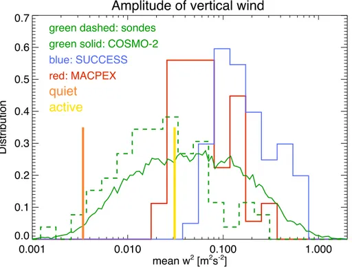
To further assess the representation of vertical velocitiesw in the COSMO-2 model,

we investigated 71 ballon soundings conducted from Payerne and the vicinty of Zurich

20

in the years 2010–2014 (see green dashed histogram in Fig. 5). We follow the work

by (Gallice et al., 2011), who showed that information on air vertical motion w can

be derived from the ascent rate of sounding balloons. The deviation of the observed ascent of a sounding balloon from the one expected in vertically quiet air, as derived from a detailed treatment of the balloon motion, is caused by the vertical motion of

25

the air w. Much simplified, but agreeing in general with this work, w can be

(18)

ACPD

15, 7535–7584, 2015

clouds

Title Page

Tables Figures

◭ ◮

Back Close

Full Screen / Esc

Discussion

P

a

per

|

Discussion

P

a

per

|

Discussion

P

a

per

|

Discussion

P

a

per

|

derive PSDs from sonde measurements since sondes measure the vertical wind vari-ance only along quasi-vertical paths in very limited regions. Rather, for comparison we

constructed a COSMO-2-based climatology of the vertical velocity variancew2 over

the Alpine region for the years 2010–2014. For this we used hourly domain-averaged

(COSMO-2, i.e., Alpine region) values ofw2 at altitudes between approximately 7 and

5

9 km. Both data sets are depicted together with the SUCCESS and the MACPEX cam-paign data in Fig. 5. The vertical velocity variance derived from the COSMO-2 analysis

and the balloon sounding agree very well, showingw2 in the range 10−3 to 2 m2s−2.

This range corresponds very well to previous observational data reporting vertical

ve-locity variances between 0.005 to 0.4 m2s−2 (Ecklund et al., 1986; Gage et al., 1986).

10

In contrast, only variances larger than about 0.02 m2s−2 were observed during the

SUCCESS- and the MACPEX campaigns. The reason for this discrepancy remains unclear, but possibly SUCCESS and MACPEX sampled mainly active periods, while the balloon data set covers quiet and active days.

We conclude from this comparison that the COSMO-2 model is able to simulate

15

a reasonable climatological distribution of vertical velocity variances, though the vertical velocity variance of individual days may be underestimated due to the missing sub-grid scale vertical motions. The power density at the unresolved frequencies higher than

10−3s−1is much lower than at smaller frequencies and hence has only a small impact

on thew2-distribution in Fig. 5. A future study should perform an in-depth evaluation of

20

the model performance on a day-by-day basis using vertical velocity measurements. The mean vertical velocity variance over the Alpine region for the day thoroughly an-alyzed in this paper is indicated by an orange line in Fig. 5: compared to the climato-logical distribution this day belongs clearly to the rather very quiet days. In addition the vertical velocity variance of an active day is shown by the yellow line. This active day is

25

further discussed in the Appendix.

The comparison of the w PSD from COSMO-2 simulations and from ALPEX

sug-gests that the spectral densities up to a frequency of about 6–8×10−4s−1 are well

(19)

ACPD

15, 7535–7584, 2015

clouds

Title Page

Tables Figures

◭ ◮

Back Close

Full Screen / Esc

Discussion

P

a

per

|

Discussion

P

a

per

|

Discussion

P

a

per

|

Discussion

P

a

per

which power density biases due to the spatial resolution of the COSMO-2 model would

be expected to be small. Higher frequency fluctuations, which may affect cirrus cloud

formation, are, however, not represented in the trajectory data and have to be added artificially. To tackle this issue, we take a similar approach as previous studies dealing with this issue (e.g., Hoyle et al., 2005; Brabec et al., 2012; Rolf et al., 2012;

En-5

gel et al., 2013; Cirisan et al., 2014): high-frequency temperature fluctuations, which are constructed from a measured PSD, are superimposed at random phase on the trajectory’s temperature time series. To construct proper small-scale temperature fluc-tuations the mean PSD of the MACPEX and SUCCESS campaign is fitted to the power

spectral density from the trajectory data at a frequency of 8×10−4s−1 (Fig. 3). The

10

high-frequency part of this scaled PSD is then Fourier transformed using 20 di_ff

er-ent random phase time series resulting in 20 different small-scale temperature series,

which are subsequently superimposed on the original temperature series. The result-ing PSD of temperature along the trajectories is shown in Fig. 3 by the orange lines

(online trajectories) and the cyan lines (offline trajectories based on 5 min wind field

15

data).

4 Cirrus cloud modeling

By means of the microphysical box model ZOMM forced by (p,T)-time series from

the introduced trajectory data sets we assess the implications of temporal resolution (Sect. 4.1), small-scale temperature fluctuations (Sect. 4.2), initial moisture content

20

(20)

ACPD

15, 7535–7584, 2015

clouds

Title Page

Tables Figures

◭ ◮

Back Close

Full Screen / Esc

Discussion

P

a

per

|

Discussion

P

a

per

|

Discussion

P

a

per

|

Discussion

P

a

per

|

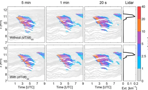
4.1 Influence of the temporal resolution of the trajectory data

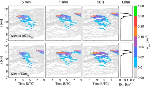
The ice water content and ice crystal number density simulated by ZOMM are shown in

Figs. 6 and 7 for different trajectory data-sets: the upper row shows simulations results

using directly the online trajectory data (right panel) and o_ffline trajectories at a

tempo-ral resolution of 1 min (middle panel) and 5 min (left panel). Both offline trajectory data

5

sets have been computed with wind field data at a temporal resolution of 5 min. The

different lines in each panel display the vertical position of each trajectories in the 10 h

prior to their arrival at the Jungfraujoch (at the right edge of each panel), while the color coding shows the modeled ice water content (Fig. 6) or the ice crystal number density (Fig. 7). Both figures show results from simulations with homogeneous nucleation only

10

and a slightly reduced initial moisture content compared to the COSMO-2 data (95 %), as no cirrus cloud occurs above Jungfraujoch in simulations using the unmodified initial moisture content. The lower rows in both figures show simulations with superimposed small-scale temperature fluctuations and will be discussed in the next section.

All simulations display a first nucleation event about 7–8 h before the arrival at

15

Jungfraujoch, but all ice particles formed in this event sediment out before the air par-cel reaches Jungfraujoch (Fig. 6). In the model runs using trajectories with a temporal resolution of 1 min and 20 s (left and middle panel) a second nucleation occurs about 2 h before the arrival at Jungfraujoch. The ice crystals nucleated in this event reach the Jungfraujoch at altitudes between 10.5 and 11.5 km, which corresponds to the

ob-20

served cloud height in the Lidar measurements (Fig. 1), as also shown by the rightmost panel in Figs. 6 and 7. The ice water content and the ice crystal number density is slightly larger in simulations based on online trajectories (rightmost panels in Figs. 6 and 7). A closer examination of this nucleation event shows that the nucleation oc-curs slightly earlier in the online trajectories data-set. Accordingly the cooling rates are

25

(21)

ACPD

15, 7535–7584, 2015

clouds

Title Page

Tables Figures

◭ ◮

Back Close

Full Screen / Esc

Discussion

P

a

per

|

Discussion

P

a

per

|

Discussion

P

a

per

|

Discussion

P

a

per

The reason for these differences are likely small differences in the removal of water

vapor after the first nucleation event and slight temporal shifts in the ascent of the

par-cel related to the different temporal resolution of the wind fields. The important second

nucleation event does not occur in simulations using trajectories at a temporal resolu-tion of 5 min.

5

SAL metric.The extinction profiles from the three simulations are shown by the green

lines in Fig. 9. The model extinction profiles compare well with the extinction profile retrieved from the Lidar measurement (black lines) in terms of the amplitude as well as in the vertical positioning of the cloud for trajectory data at a temporal resolution of 20 s and 1 min (Fig. 8b and c). Accordingly the location, amplitude and structure error

10

in the SAL metric are small for all simulations (see orange upward-pointing triangles in Fig. 10 below). In contrast, no cloud forms above Jungfraujoch in simulations with trajectories with 5 min temporal resolution (Fig. 8a).

4.2 Influence of small scale temperature fluctuations

Small-scale temperature fluctuations, which are not resolved in the NWP model, can

15

modify the cooling rate at the time of nucleation and therefore alter the number of nucleated ice crystals in case of a homogeneous nucleation event. To assess the im-pact of these temperature fluctuations we superimposed additional temperature fluc-tuations, which are derived from measurements during the SUCCESS- and MACPEX-campaigns on the original trajectory temperature series (Sects. 3.2 and 3.3). The

influ-20

ence of this modification of the temperature series on the microphysical evolution can be seen by comparing the upper and lower rows of Figs. 6 and 7. The influence on the corresponding extinction profile is shown by the grey lines in Figs. 8 and 9 (compare to green line). From these figures it is obvious that the added temperature fluctuation have a significant impact on the modeled extinction profiles if trajectories are used at minute

25

(22)

ACPD

15, 7535–7584, 2015

clouds

Title Page

Tables Figures

◭ ◮

Back Close

Full Screen / Esc

Discussion

P

a

per

|

Discussion

P

a

per

|

Discussion

P

a

per

|

Discussion

P

a

per

|

profile (Fig. 9a). The physical reason for the strongly different impact of superimposed

temperature fluctuations for online trajectories and 1 min trajectories is not evident from our analysis as the temperature PSDs and the initial conditions for both trajectory sets are almost identical. This issue needs to be addressed in a future study.

SAL metric. In terms of the SAL metric, the influence of the additionally

superim-5

posed small-scale temperature fluctuations influences particularly the amplitude of the modelled extinction profile (open and filled symbols in Fig. 10 below). In general, the

lo-cation and shape of the cloud (L-component) is not positively affected by adding

small-scale temperature fluctuations. Consistent with the previous discussion the impact is largest for simulations with a small temporal resolution of the trajectory data.

10

4.3 Influence of variations in the initial moisture content

As it is known that the moisture content in weather prediction models are very uncertain

in the upper troposphere (Kunz et al., 2014), simulations with different specific humidity

at the trajectory starting points were performed. We used initial humidities between 90 and 110 % of the values calculated by the COSMO-2 model. The extinctions resulting

15

from these sensitivity runs are shown in Fig. 8 (assuming homogeneous nucleation

only). Offline trajectories with a temporal resolution of 1 and 5 min are displayed in

panels a and b. Simulations using online trajectories are displayed in panel c. For the

simulations using online trajectories, all runs except the+5 and+10 % cases display

a cloud at the right altitude with very good agreement with the measured extinction

20

profiles. The enhanced humidity cases produce clouds at a too low altitudes because of a too early nucleation and subsequent sedimentation of the formed ice crystals.

For the offline trajectories with a temporal resolution of 5 min, the variation of the

initial humidity leads in almost all cases to a disappearance of the cloud (Fig. 8c).

Using offline trajectories with a temporal resolution of 1 min (Fig. 8b) results in profiles

25

similar to the ones using online trajectories.

SAL metric.The conclusion that increasing temporal resolution of the trajectory data

(23)

ACPD

15, 7535–7584, 2015

clouds

Title Page

Tables Figures

◭ ◮

Back Close

Full Screen / Esc

Discussion

P

a

per

|

Discussion

P

a

per

|

Discussion

P

a

per

|

Discussion

P

a

per

decreasing importance of the unresolved small-scale temperature fluctuations hold for

any initial humidity modification investigated. However, the differences between

simu-lations with different initial humidities are very large. While all terms in the SAL metric

are influenced by changes in the initial humidity, the impact on the cloud location is particularly large (Figs. 8 and 10).

5

4.4 Influence of the ice nuclei number density

An additional uncertainty in modeling the microphysical evolution of cirrus clouds is the

potential presence of ice nuclei (IN). These can affect the microphysical evolution as

they influence the supersaturation and temperature required for nucleation. Further, IN

can lead to a reduction of the nucleated ice crystal number density, which may affect

10

the sedimentation velocity of the ice crystals and hence the total water content of the respective air parcel.

We performed simulations including heterogeneous nucleation on different IN

con-centrations. Significant differences can be observed between the results from these

simulations even for a single trajectory data set (Fig. 9). The general finding is that

15

simulations with 0, 10 or 20 IN L−1 show good agreement with observations, with

differences amongst each other smaller than uncertainties due to unresolved

small-scale temperature fluctuations and smaller than uncertainties in the observations.

Con-versely, simulations with more than 20 IN L−1 do not provide good agreement with

ob-servations.

20

In the case of online trajectories (20 s) the almost complete loss of extinction for IN

concentration of 100 L−1is due to a fast evaporation of ice crystals, once they enter the

subsaturated region below about 10 km a.s.l. However, this is not a very robust feature,

because the 1 and 5 min o_ffline cases manage to let some of these particles survive,

likely due to a delicate phasing of cooling and warming along the different trajectories

25

(24)

ACPD

15, 7535–7584, 2015

clouds

Title Page

Tables Figures

◭ ◮

Back Close

Full Screen / Esc

Discussion

P

a

per

|

Discussion

P

a

per

|

Discussion

P

a

per

|

Discussion

P

a

per

|

The similarity of the extinction profiles for the simulations with only homogeneous nucleation and those with low IN concentrations is linked to the very fast sedimentation of the ice crystals forming in the early phase of the simulated 10 h time period. The very fast sedimentation of the ice crystals allows for multiple nucleation events along the trajectory and these gradually remove all IN from the air parcel. Hence the last

nu-5

cleation leading to the cloud present at arrival above Jungfraujoch is formed exclusively by homogeneous nucleation.

The simulations using offline trajectories at 5 min resolution (Fig. 9a) show a very

different behavior for the simulation with 10 L−1: the formed cloud sediments out

be-fore reaching Jungfraujoch and no second nucleation event occurs. Using the

of-10

fline trajectories without superimposing temperature fluctuations, the model produces

a cloud only when assuming an IN concentration of 20 L−1. For simulations using

IN-concentrations larger than 50 L−1, clouds only exist at lower levels. However, if we use

o_ffline trajectories with a temporal resolution of 1 min, the model results resemble again

those using online trajectories (Fig. 9b).

15

SAL metric. While there is clearly a strong impact of the assumed nucleation mode

and the IN number density on the microphysical evolution, its influence may vary in a non-linear fashion with other uncertainties, such as variations in the initial humidity. This becomes also clear from the SAL-analysis shown in Fig. 10: the comparison of

di_fferent symbols with the same color indicates no consistent improvement for a single

20

nucleation mode in any of the three error components.

Similarly to the experiments with modified initial moisture content, the assumed IN

number density does not a_ffect the conclusions on the importance of small-scale

tem-perature fluctuations and increasing temporal resolution of the trajectory data. Adding

small IN number densities (≤20 L−1) has little effect on the simulated extinction profiles

25

for trajectories with a high temporal resolution, while adding 50 L−1or more significantly

(25)

ACPD

15, 7535–7584, 2015

clouds

Title Page

Tables Figures

◭ ◮

Back Close

Full Screen / Esc

Discussion

P

a

per

|

Discussion

P

a

per

|

Discussion

P

a

per

|

Discussion

P

a

per

5 Conclusions

An analysis of the uncertainties involved in Lagrangian cirrus modeling has been

pre-sented. The investigated sensitivities include the effects of (i) the temporal resolution

of the trajectory data and of the underlying wind fields (20 s to 1 h), (ii) the superposi-tion of unresolved small-scale temperature fluctuasuperposi-tions, (iii) small perturbasuperposi-tions to the

5

specific humidity at the trajectory starting points (±10 %), and (iv) different ice nuclei

concentrations.

The temporal resolution of the wind field data has a pronounced impact on vertical velocities and therefore the temperature variance captured in the trajectory data. To capture most of the variability that is represented in NWP models with a horizontal grid

10

spacing of 2.2 km, trajectory data should be used at least at a 5 min temporal resolution. For the cirrus cloud investigated in this study, the modeled extinction profile matches very well with the observations if trajectory data is used at a temporal resolution of 1 min or higher and using wind field data at a resolution of 5 min or higher.

Vertical velocity fluctuations occurring at highest frequencies are not resolved in

15

state-of-the-art numerical weather prediction model due to the finite grid resolution. Yet, tese high frequency fluctuations may alter the cooling rates locally and thus in-fluence ice nucleation events. To investigate the impact of the unresolved fluctuations we superimposed onto the original temperature series the missing frequencies of the temperature fluctuations, which are derived from observed power spectral densities of

20

temperature fluctuations from the SUCCESS and MACPEX campaigns. (The

observa-tional PSD are scaled to the model PSD at the cut-offfrequency to obtain a continuous

PSD.) The influence of these superimposed temperature fluctuations is significant for trajectories with a temporal resolution of 5 min and successively decreases for trajec-tories with a temporal resolution of 1 min and 20 s, respectively. While the modelled

25

(26)

ACPD

15, 7535–7584, 2015

clouds

Title Page

Tables Figures

◭ ◮

Back Close

Full Screen / Esc

Discussion

P

a

per

|

Discussion

P

a

per

|

Discussion

P

a

per

|

Discussion

P

a

per

|

at temporal resolution of 1 or 5 min. In the Appendix we show that the imposed small scale temperature fluctuations have significant impact on the cirrus clouds both for the

quiet and active periods i.e., with strongly different vertical velocity variances, using 1 h

wind data and 1 min trajectory temporal resolution (Fig. 14). Even for a regional model with 2.2 km resolution, the superposition of small-scale temperature fluctuation should

5

be considered in cirrus simulations.

In order to obtain physically meaningful small-scale temperature fluctuations some assumption about the shape and amplitude of the power spectral density of the ver-tical velocity and temperature are required. A comparison of the PSD and variance of the vertical velocity predicted by the COSMO-2 model for the present case study

10

shows significant di_fferences to observational data from the SUCCESS and MACPEX

campaigns, which have been used previously to superimpose small-scale temperature

fluctuations. Significant differences in the wave energy occur even for low-frequency

waves with wavelength on the order of 100 km, which should not be a_ffected by the

grid resolution. However, the modeled PSD agrees well with those observed during

15

quiet days in the ALPEX-campaign. Further indication of a large day-to-day variability of the vertical velocity variance is provided by the analysis of balloon sounding data from the Alpine region. A climatological analysis of the vertical velocity variance in the COSMO-2 analysis suggests that the model can capture the entire range of observed vertical velocity variance. However, future studies should perform an in-depth

evalua-20

tion of the model capability to predict the vertical velocity PSD for different regions and

large-scale meteorological conditions.

The specific moisture content at the starting point of each trajectory determines the absolute values of saturation with respect to ice. We observe significant changes in the modeled cirrus cloud properties and microphysical evolution if the initial specific

25

humidity is varied by ±10 % of the model value. For high-resolution trajectory data