Three-Dimensional Spectral-Domain Optical Coherence
Tomography Data Analysis for Glaucoma Detection
Juan Xu1., Hiroshi Ishikawa1,2., Gadi Wollstein1
*, Richard A. Bilonick1, Lindsey S. Folio1,2, Zach Nadler1, Larry Kagemann1,2, Joel S. Schuman1,2
1University of Pittsburgh Medical Center (UPMC) Eye Center, Eye and Ear Institute, Ophthalmology and Visual Science Research Center, Department of Ophthalmology, University of Pittsburgh School of Medicine, Pittsburgh, Pennsylvania, United States of America,2Department of Bioengineering, Swanson School of Engineering, University of Pittsburgh, Pittsburgh, Pennsylvania, United States of America
Abstract
Purpose:To develop a new three-dimensional (3D) spectral-domain optical coherence tomography (SD-OCT) data analysis method using a machine learning technique based on variable-size super pixel segmentation that efficiently utilizes full 3D dataset to improve the discrimination between early glaucomatous and healthy eyes.
Methods:192 eyes of 96 subjects (44 healthy, 59 glaucoma suspect and 89 glaucomatous eyes) were scanned with SD-OCT. Each SD-OCT cube dataset was first converted into 2D feature map based on retinal nerve fiber layer (RNFL) segmentation and then divided into various number of super pixels. Unlike the conventional super pixel having a fixed number of points, this newly developed variable-size super pixel is defined as a cluster of homogeneous adjacent pixels with variable size, shape and number. Features of super pixel map were extracted and used as inputs to machine classifier (LogitBoost adaptive boosting) to automatically identify diseased eyes. For discriminating performance assessment, area under the curve (AUC) of the receiver operating characteristics of the machine classifier outputs were compared with the conventional circumpapillary RNFL (cpRNFL) thickness measurements.
Results:The super pixel analysis showed statistically significantly higher AUC than the cpRNFL (0.855 vs. 0.707, respectively, p = 0.031, Jackknife test) when glaucoma suspects were discriminated from healthy, while no significant difference was found when confirmed glaucoma eyes were discriminated from healthy eyes.
Conclusions:A novel 3D OCT analysis technique performed at least as well as the cpRNFL in glaucoma discrimination and even better at glaucoma suspect discrimination. This new method has the potential to improve early detection of glaucomatous damage.
Citation:Xu J, Ishikawa H, Wollstein G, Bilonick RA, Folio LS, et al. (2013) Three-Dimensional Spectral-Domain Optical Coherence Tomography Data Analysis for Glaucoma Detection. PLoS ONE 8(2): e55476. doi:10.1371/journal.pone.0055476
Editor:Pedro Gonzalez, Duke University, United States of America
ReceivedSeptember 19, 2012;AcceptedDecember 23, 2012;PublishedFebruary 11, 2013
Copyright:ß2013 Xu et al. This is an open-access article distributed under the terms of the Creative Commons Attribution License, which permits unrestricted use, distribution, and reproduction in any medium, provided the original author and source are credited.
Funding:This work was supported by National Institutes of Health (NIH R01-EY013178; R01-EY011289; P30-EY008098), http://grants.nih.gov/grants/oer.htm; and the Eye and Ear Foundation (Pittsburgh, Pennsylvania, United States of America), http://www.eyeandear.org/; and Research to Prevent Blindness (http://www. rpbusa.org/rpb/). The funders had no role in study design, data collection and analysis, decision to publish, or preparation of the manuscript.
Competing Interests:The authors have the following interests: JSS receives royalties for the following intellectual property licensed by Massachusetts Institute of Technology to Carl Zeiss Meditec - Method and apparatus for optical imaging with means for controlling the longitudinal range of the sample, Issued on June 14, 1994, U.S. Patent No. 5,321,501. There are no further patents, products in development or marketed products to declare. This does not alter the authors’ adherence to all the PLOS ONE policies on sharing data and materials.
* E-mail: [email protected]
.These authors contributed equally to this work.
Introduction
Optical coherence tomography (OCT) is a rapidly evolving technology and has gained a significant clinical impact in ophthalmology.[1–4] One of the major OCT applications is glaucoma assessment by measuring retinal nerve fiber layer (RNFL) thickness in circumpapillary and macula regions. Many studies showed that the current OCT quantitative assessment has excellent glaucoma discriminating ability. [1,3,5,6].
Spectral-domain (SD-) OCT’s fast scanning speed allows three-dimensional (3D) volume scanning of the retina, which may offer detailed and accurate quantitative analysis of the retinal structure. However, despite the rich information embedded in 3D OCT
images, current standard quantitative structural OCT measure-ment is mostly limited to several hundred sampling points along a 3.4 mm circle diameter centered at optic nerve head, which does not take full advantage of the 3D dataset (over 20,000 sampling points). This sampling pattern was chosen mostly to allow compatibility with legacy data obtained using time-domain (TD-) OCT. The limited tissue sampling might lead to situations where early signs of structural changes are not detected when located outside the sampled circle (Fig. 1).
thickness within a fixed number of neighboring sampling points (fixed-number super pixels) and comparing this measurement with age-matched normative databse. However, there is no quantitative summary of this super pixel analysis, and therefore clinicians’ subjective interpretation is required.
In the clinical practice, subjects are often classified into three major groups: healthy, glaucoma suspect or glaucoma. Classifying subjects as ‘‘suspect’’ has important clinical advantage because some of these subjects posses pre-perimetric glaucoma character-istics. With the paucity of functional indication of glaucoma, correctly identifying glaucoma suspect based on their structural features is of upmost importance as it would allow timely adjustemt of clinical management. However, detection of pre-perimetric disease is still posing a significant challenge. [7,8] We hypothesize that a comprehensive use of the full 3D OCT data would improve detection of early glaucoma. The purpose of this study was to develop a novel 3D SD-OCT data analysis technique utilizing the full 3D dataset to improve the ability to detect glaucomatous structural damage at early stages. The new method uses variable-size super pixel mapping with a machine classifier analysis to quantitatively assess the full 3D OCT data. Unlike the conventional super-pixel analysis, which uses a fixed number of points, the newly developed variable-size super pixel is defined as a cluster of homogeneous adjacent pixels with variable size, shape and number. In this paper, we investigate whether the variable-size super pixel analysis is better suited for handling individual eye characteristics that might lead to improved glaucoma diagnosis predominantely in early disease stage.
Methods
Ethics Statement
This study was obtained the Institutional Review Board (IRB) approval named ‘‘Optical Coherence Domain Reflectometry and Optical Coherence Tomography Measurements of Intraocular Structure’’.
Subjects and Image Acquisition
This study was conducted with healthy, glaucoma suspect and glaucomatous eyes with a wide range of disease severity selected from the Pittsburgh Imaging Technology Trial (PITT). One hundred and ninety-two eyes of 96 subjects (44 healthy, 59 glaucoma suspect and 89 glaucomatous eyes) were enrolled to test the glaucoma discrimination performance. An independent dataset, including 46 eyes of 46 healthy subjects (randomly selected one eye for each subject), was used as the normative database. Institutional Review Board (IRB) approval was obtained for the study and all participants gave their consent to participate in the study. The study adhered to the Declaration of Helsinki and Health Insurance Portability and Accountability Act regulations.
Exclusion criteria for the study included history of ocular trauma or surgery (except for uncomplicated cataract or glaucoma surgery) and disease or treatment that might affect the visual field (e.g., stroke, central nervous sytem tumors) or retinal thickness (diabetes melitus, chronic steroid treatment).
All subjects had a comprehensive ophthalmic evaluation, reliable visual field (VF) and 3D SD-OCT scan all acquired
within 6 months of each other. The ophthalmic evaluation included medical history, best-corrected visual acuity, manifest refraction, intraocular pressure (IOP) measurement, gonioscopy, slit-lamp examination before and after pupil dilation, and VF testing. VF was considered reliable if false negatives, false positives and fixation losses were less than 30%. All subjects had 3D OCT scans centered at the optic nerve head (ONH) (Cirrus HD-OCT;
Carl Zeiss Meditec, Inc., Dublin, CA; ONH cube 2006200 scan
protocol).
Clinical Diagnosis
Eyes were defined as healthy if there was no history of
glaucoma, IOP#21 mmHg, the ONH did not meet the criteria
for glaucomatous optic neuropathy (GON), as described below, and VF was normal.
Eyes were defined as glaucomatous if there was both GON and glaucomatous VF loss. GON was defined if either one of the following criteria was met: inter eye cup-to-disc (C/D) ratio
asymmetry .0.2, accounting for disc size; rim thinning or
notching; cup to disc ratio $0.6; RNFL wedge defect or disc
hemorrhage. Glaucomatous VF was diagnosed if any of the following findings were evident on two consecutive VF tests: a glaucoma hemifield test outside normal limits, pattern standard
deviation (PSD) ,5%, or a cluster of three or more non-edge
points in typical glaucomatous locations (arcuate scotoma, nasal step, paracentral scotoma or temporal wedge), all depressed on the
pattern deviation plot at a level of p,0.05, with at least one point
in the cluster depressed at a level of p,0.01.
Glaucoma suspect eyes had IOP between 22 to 30 mmHg and/ or GON features all in the presence of a normal VF test.
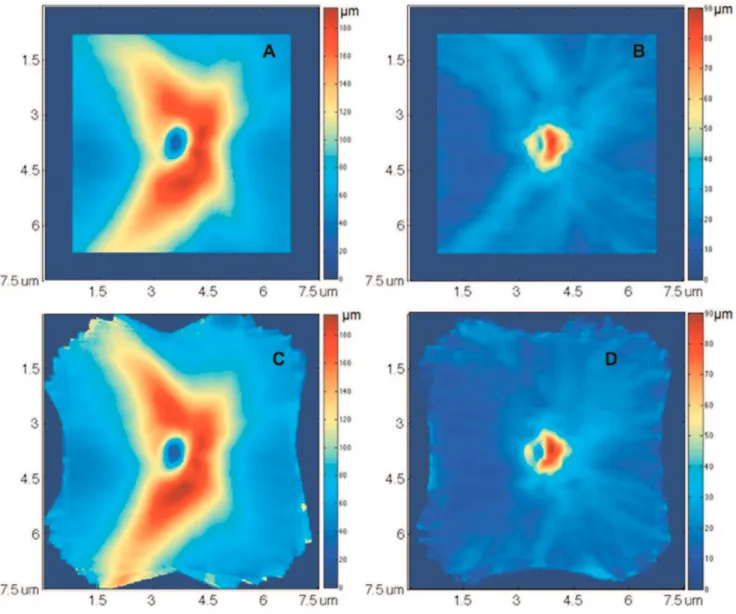
Figure 2. Normative database normalization with 46 healthy eyes.(A, B) mean and standard deviation (SD) of retinal nerve fiber layer (RNFL) thickness measurement at each sampling point (A-scan), without normalization. (C, D) mean and SD of RNFL thickness measurement after normalizing individual’s retinal nerve fiber bundle path location to population’s average location. The variations of RNFL thickness were larger at superior temporal and inferior temporal regions (brighter blue in B) because of the population variation of the bundle locations. After aligning the bundle locations and normalizing the RNFL thickness map, the RNFL thickness variations at these two regions were markedly reduced (dark blue in D).
doi:10.1371/journal.pone.0055476.g002
3D SD-OCT Data Analysis
Super pixel mapping is a partitioning of image into a number of close-to-homogenous segments with variable sizes and shapes. The features of these variable-size super pixels were then extracted and used as the input for machine classifier analysis in order to generate a key index output for each image. The procedure to generate the index output included the following steps: compar-ison with normative database, feature map generation, super pixel mapping, feature extraction, and classification.
1. Normative Database. A normative database was assem-bled to measure the RNFL thickness deviation at each sampling point in the 3D dataset. Retinal layer segmentation, which was optimized for 3D SD-OCT dataset [9] was applied on each 3D OCT image to obtain the RNFL thickness and reflectivity at every
single sampling point (total 2006200 points). All segmented 3D
OCT datasets were visually evaluated to ensure the correct
segmentation. Any OCT scan with.8% consecutive B-scan from
the total number of B-scans that showed segmentaion error or
.12% cumulative segmentation error was excluded from the
study. ONH margin was automatically detected on the OCT fundus image using a software program of our own design. [10] Major retinal nerve fiber bundle path at each hemi-field on each RNFL thickness map was automatically detected. Each RNFL thickness map was then normalized by aligning the bundle location at each hemi-field to a reference position (population’s average bundle location) for the comparison with the normative database in order to minimize spatial variability in RNFL thickness, especially at superior temporal and inferior temporal regions (Fig. 2). The RNFL thickness map normalization was processed on the concentrated circles with different radii started from the ONH center. For each subject, the ONH center was first aligned at a reference center point. At each concentrated circle, two average bundle location (superior and inferior) were computed from the normative database. Each subject’s RNFL thickness profile at the given circle was normalized by strenching/shrinking so the subject’s bundle location would coincide with the population average bundle location. The entire RNFL thickness
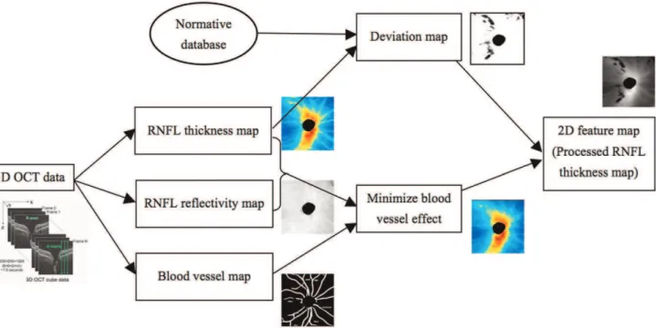
Figure 3. Flowchart of converting a 3D OCT image into a 2D feature map.
doi:10.1371/journal.pone.0055476.g003
Figure 4. Super pixel segmentation on 3D OCT images.(A) Analysis output in a healthy eye, (B) glaucoma suspect, and (C) glaucomatous eye. Abnormally thin retinal nerve fiber layer is marked with small super pixels.
map was normalized by repeating this process at all concentrated circles.
2. 2D Feature Map Generation. Each 3D OCT image
(200620061024 voxels) was converted to a 2D feature map
(2006200 pixels) as follows. RNFL thickness and reflectivity along
Table 1.Super pixel features used as inputs for the machine learning classifier.
Super Pixel Features Healthy Glaucoma Suspect Glaucoma
Number of super pixels Total number of super pixels 151.8659.5 187.5664.4 250.8659.4 Total number of small super pixels with
‘‘Tmin,size,T1’’
66.1654.0 97.0655.1 150.9654.3
Total number of super pixels with ‘‘size.T2’’ 40.5614.3 31.3614.7 18.3611.9
Numbers of super pixels with the RNFL thickness at pre-defined ranges:
0–30mm 41.4653.0 67.1656.4 139.3675.8
75–120mm 26.367.4 26.667.0 16.569.6
120–165mm 4.563.1 1.462.0 0.661.2
Numbers of super pixels with the size at pre-defined ranges:
30–120 pixels 65.9654.0 98.1656.0 152.7653.5
360–420 pixels 7.164.4 5.063.3 3.762.5
420–540 pixels 15.467.6 11.566.5 6.564.4
Mean, Standard deviation, 3rdand 4th central moments
Super pixel RNFL thickness
55.9615.1mm 48.2612.9mm 34.8610.9mm
27.464.0mm 24.9962.8mm 21.864.0mm
0.960.3 0.8960.2 1.1960.4
3.260.8 3.1960.7 4.2961.8
Super pixel size
288.86102.9 231.1691.5 163.3650.5
204.2642.9 191.3653.2 141.9654.3
0.961.2 1.761.1 2.560.8
4.864.3 7.165.2 11.866.3
Super pixel RNFL thickness with ‘‘Tmin,size,T1’’
47.1622.8mm 40.0616.0mm 26.669.2mm
21.767.5mm 21.266.6mm 17.663.9mm
1.360.8 1.460.6 1.860.5
5.463.4 5.562.3 7.763.0
Super pixel RNFL thickness with ‘‘size.T2’’
70.9611.7mm 65.268.6mm 52.3613.1mm
27.065.5mm 22.863.5mm 18.167.0mm
0.660.2 0.660.4 0.860.5
2.460.4 2.660.8 2.961.3
Distributions The value of each bin in the normalized histogram distribution of super pixel RNFL thickness
Figure 5A Figure 5A Figure 5A
The value of each bin in the normalized histogram distribution of super pixel size
Figure 5B Figure 5B Figure 5B
Average RNFL thickness Thickness at 3.4mm circle 105.3618.6mm 96.1615.5mm 72.3619.3mm Thickness at entire scan region 89.5615.9mm 79.0613.3mm 61.8615.1mm
Thickness at entire scan region excluding ONH region
88.0615.6mm 78.4613.5mm 61.1615.2mm
Data reported as Mean6SD.
Tmin,T1, T2– Thresholds of minimal super pixel size, small super pixel size and large super pixel size respectively, RNFL – retinal nerve fiber layer, ONH – optic nerve head.
doi:10.1371/journal.pone.0055476.t001
with the blood vessel mapping were extracted from each image (Fig. 3). The normalized RNFL map after applying the bundle path correction were compared with the normative database point by point to obtain a deviation map, with the cut-off value set to mean value minus stardard deviation (SD). Unlike the conven-tional setting of cut-off value, i.e., mean value - 2SD in most OCT devices, this new setting is more sensitive to identify the case at the border of the normative database, which might be an indicator of the structural changes at the early stage. With this new setting, the RNFL data lower than the bottom 15.9% of the normative database was set with higher probability for the further process, comparing with the bottom 2.3% using the conventional setting. The internal reflectivity of retinal nerve fiber layer has been proved to be useful in glaucoma assessment. [11] The RNFL internal reflectivity, was calculated by taking the average reflectivity within the RNFL along each A-scan, with each voxel’s reflectivity normalized to its A-scan’s saturation before the averaging. Retinal blood vessel generated shadow at retina nerve fiber layer, which was noise in the RNFL thickness computation. Moreover, the vessel patterns varied randomly among subjects. To minimize the vessel effect on the RNFL thickness map, the retinal blood vessels in the 3D dataset were automatically detected using a 3D boosting algorithm [12] and filled out. The RNFL thickness of each pixel located at the blood vessel region was replaced by a value computed from all the non-vessel pixels on the RNFL
thickness map using bi-linear interpolation. The final feature map is a function of the RNFL thickness and interal refleciviy after accounting for the blood vessls and the deviation map.
3. Variable-size super pixel segmentation. Variable size/ shape super pixels were automatically mapped on the 2D feature map by grouping homogeneous neighboring pixels using a ncut algorithm. [13] The ncut algorithm is to partition an image into dozens to thousands of small regions (called super pixels) by grouping neighboring pixels, where pixels within a partitioned region have homogenous properties while different partitioned regions have maximal differences in their properties. One hundred super pixels were initially segmented on the feature map. The size of each super pixel was automatically adjusted with the pre-defined criteria based on the pathologic contexts of glaucoma. To be more sensitive to RNFL thinning (glaucomatous damage), smaller super pixels were assigned to thinner RNFL. Each initially
segmented super pixel was recursively partitioned into N more
super pixels, whileNwas a function of mean, standard deviation,
size, and deviation to the normative database of the given super pixel compared with global mean and standard deviation of the 2D feature map, written as:
N~
1, if h(Zsp,ssp,Nsp,Devsp)~1
a1(Zmax{Zsp)=(Zmax{Zavg)|(Nsp=Nmin),
if h(Zsp,ssp,Nsp,Devsp)~0and Zsp§Zavg
a2(Zavg{Zsp)=Zavg|(Nsp=Nmin),
if h(Zsp,ssp,Nsp,Devsp)~0and ZspvZavg 8
> > > > > > > > <
> > > > > > > > :
ð1Þ
where Zsp,ssp,Nsp,Devsp represented the average RNFL
thick-ness, RNFL standard deviation, size and average deviation of the
given super pixel,Nmin was a pre-defined minimal size of super
pixel,ZavgandZmaxwere the average and maximal thickness with
the entire 2D RNFL thickness map.hwas defined with a series of
criteria with ‘‘IF’’, ‘‘logical AND’’, ‘‘logical OR’’ and ‘‘logical NOT’’ operations, which corresponded to different super pixel conditions need further partition or not, written as:
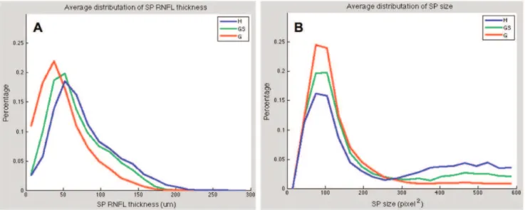
Figure 5. Normalized histogram distribution of super pixel.(A) RNFL thickness and (B) super pixel size for healthy (H), glaucoma suspect (GS), and glaucomatous (G) eyes.
doi:10.1371/journal.pone.0055476.g005
Table 2.Characteristics of the study participants.
Healthy n= 44
Glaucoma Suspect n= 59
Glaucoma
n = 84 p-value Age (years) 54.868.9 61.969.6 66.968.7 ,0.001*
Male/female 5/18 13/24 21/30 0.269{
MD (dB) 20.0961.28 20.4561.64 25.8865.80 ,0.001{
Values are means6standard deviation.
MD – visual field mean deviation, * –ANOVA with linear model,{
– Chi square test,{– ANOVA with mixed effects models.
h~
0, if (Zspw1:1|Zavg),and(Nspw2|Nmin),
and(Devspv0:95)and(ssp§0:2|savg)
0, if (ZspvZavg),and(NspwNmin),and(Devspv0:95)
1, Otherwise
8 > > > > > <
> > > > > :
ð2Þ
a1 anda2were two constants chosen based on the segmentation
logic, which were used to control the number of segments
partitioned in the given super pixel. Fora1, because super pixel
RNFL thickness was thicker than the average RNFL thickness, this
super pixel was further partitioned only if its standard deviation was large enough. We wanted the super pixel partitions into several big segments, and recursively partitions into small segments in the following iterations. Therefore,a1was set to 0.2 to lower the
number of the segments. For a2, since the super pixel RNFL
thickness was thinner than the average RNFL thickness, we wanted to partition the super pixel into many small segments.
Therefore,a2was set to 1.2 to higher the number of segments.
The stability is an important parameter in ncut algorithm to control the super pixel segmentation result. It was set to a small
value, i.e., 20.1, to let the 100 initial super pixels have more
flexible boundaries. In the recursive partition processing, to make
Figure 6. The receiver operating characteristic curves (ROCs) computed with the machine classifier method and Cirrus HD-OCT software generated mean cpRNFL thickness.(H) healthy eyes, (G) glaucomatous eyes, (GS) glaucoma suspect eyes.
doi:10.1371/journal.pone.0055476.g006
the super pixels having smooth boundaries and compact shapes, the stability variable was set to a relatively large value, i.e.20.006. In summary, the super pixel number and size were automat-ically adjusted by initial segmentation and recursive partition. The segmented feature map provided a qualitative analysis with more natural representation, in which damaged areas tended to have smaller super pixels, while normal regions had larger super pixels (Fig. 4).
4. Feature Extraction. Super pixel map provided a qualita-tive representation of the structural damage. To summarize the map as quantitative disease indices, a total of 68 super pixel features were extracted and used as the inputs of machine learning classifiers analysis (Table 1). Three thresholds, Tmin, T1, and T2 were set to 50, 133, and 400 pixels respecitvely based on the experiments to obtain two sub-groups of super pixel with large size and small size. The features were calculated from all super pixels together with two sub-groups.
5. Glaucoma Classification. Glaucoma classification was performed by implementing LogitBoost adaptive boosting algo-rithm, [14] which was designed as a supervised two-class machine classifier. Because the machine classifier was a two-class classifier, only two of the three clinical groups (healthy, glaucoma suspects, and glaucoma) were used to train the classifier each time. The output of the classifier was a continuous number ranging from negative (health) to positive (disease) value. Ten-fold cross validation was used to train and test the machine classifier.
Statistical Analysis and Evaluation
The software performance was evaluated by the area under the receiver operating characteristics (AUCs) of the machine classifier outputs, for discriminating between healthy and diseased eyes.
AUCs were compared with those of the conventional method of diagnosis – the mean and best quadrant measurements of the circumpapillary RNFL (cpRNFL) thickness generated by Cirrus HD-OCT software. If both eyes had the same clinical diagnosis, one eye was randomly selected from each subject to compute AUCs. AUCs were compared using the Jackknife method, [15] which is equivalent to the method of DeLong et al. [16] Sensitivity at the 85% specificity was calculated for each of the machine classifier outputs and compared with the measurements of conventional cpRNFL analysis.
Results
One hundred and ninety-two eyes of 96 subjects (44 healthy, 59 glaucoma suspect and 89 glaucomatous eyes) qualified for the study. The characteristics of the study participants were summa-rized in Table 2. Five glaucomatous eyes (5 subjects; 5.2%) were excluded from the study due to retinal layer segmentation failure. Examples of the results of super pixel mapping are given in Fig. 4. The super pixel boundaries were superimposed on the processed grey scale RNFL thickness map, where a brighter pixel intensity corresponded to a thicker RNFL. Different super pixel distribution patterns are evident in the various stages of glaucomatous damage. The population’s average distributions of super pixel RNFL thickness and size for healthy, glaucoma suspects, and glaucomatous eyes are illustrated in Fig. 5.
Glaucoma discriminating performance was assessed with three different grouping combinations: healthy vs glaucoma+glaucoma suspects (HvGGS), healthy vs glaucoma suspects (HvGS), and healthy vs glaucoma (HvG). Table 3 gives the performance of cpRNFL thickness measurements in global and 4 quadrants. Comparing with the conventional cpRNFL thickness, machine classifier provided better AUCs and higher sensitivities (Table 4 and Fig. 6). The AUC for HvGS was statistically significantly higher with the super pixels analysis than the conventonal cpRNFL thickness (0.855 vs 0.707, respectively, p = 0.031, Jackknife test), while no significant difference was detected with HvGGS and HvG. Comparing with the best quadrant measure-ments, i.e., the inferior quadrant, the machine classifier showed higher sensitivities for HvGGS and HvGS without reaching statistical significance (Table 5).
Discussion
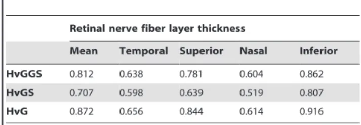
Current standard quantitative glaucoma analysis using 3D SD-OCT have substantial room for improvement especially for detection of early glaucoma. [7,8] One possible reason is that only a small fraction of the 3D dataset is used in the analysis. We suggest a new 3D OCT data analysis method, using machine Table 3.Area under the receiver operating characteristic
curves (AUCs) of conventional circumpapillary RNFL (cpRNFL) thickness measurements in global and four quadrants from Cirrus HD-OCT software.
Retinal nerve fiber layer thickness
Mean Temporal Superior Nasal Inferior
HvGGS 0.812 0.638 0.781 0.604 0.862
HvGS 0.707 0.598 0.639 0.519 0.807
HvG 0.872 0.656 0.844 0.614 0.916
HvGGS – healthy vs glaucoma+glaucoma suspects, HvGS – healthy vs glaucoma suspects, HvG – healthy vs glaucoma.
doi:10.1371/journal.pone.0055476.t003
Table 4.Area under the receiver operating characteristic curves (AUCs) computed with machine classifier and Cirrus HD-OCT software generated mean cpRNFL thickness.
cpRNFL thickness Boosting machine classifier
AUC
Sensitivity at the 85%
Specificity AUC AUC Difference{
[95% CI]
Sensitivity at the 85% Specificity
HvGGS 0.812 45.5% 0.847 0.035 [20.053, 0.122] 90.9%
HvGS 0.707 45.5% 0.855 0.148* [0.013, 0.283] 86.4%
HvG 0.872 63.6% 0.903 0.031 [20.035, 0.098] 81.8%
{
Difference with RNFL thickness AUC, * statistically significant.
learning technique based on variable-size super pixel mapping to quantitatively summarize the full 3D dataset and automatically identify glaucomatous eyes. We demonstrated that this method was better at discriminating glaucoma suspect eyes from healthy eyes (HvGS) comparing with mean cpRNFL thickness, and performed at least as well for HvG and HvGGS. The improved performance in discriminating early disease is because this method is tailored to detect localized damage that typically occurs at early stage of glaucoma. However, in late stage of the disease, a globalize damage is more common where the variably sized super pixel analysis has the same performance as the cpRNFL analysis. There are several advantages of variable size/shape super pixel machine classifier analysis. First, flexible size and shape super pixel processing provides more natural representation to fit the variable spatial architecture of the structural damages. Many ocular diseases demonstrate areas of pathologic change with measureable differences from unaffected areas when considering features such as retinal layer thickness, internal reflectivity, etc.[6,17–19] These pathologically affected areas usually share similar characteristics but with variable magnitude in variable shape and size. Therefore, variable-size super pixel segmentation efficiently depict this natural representation by grouping similar neighboring sampled points based on the homogeneity of various features. Second, super pixel processing is computationally efficient. Super pixel mapping reduces the number of data points from over 20,000 sampling points down to a few hundred super pixels by condensing the redundant information. This is a common approach for handling such a high density data with the balance of preserving meaningful information and improving the computational efficiency. More-over, machine classifier provides an efficient and optimized way to combine dozens of super pixel features together with global RNFL features into one key index to automatically identify diseased eyes. The performance of the software was based on the combination of super pixel processing and machine learning technique. Our study showed that the new super pixel analysis method quantitatively summarize the full 3D OCT dataset, which outperformed the conventional cpRNFL analysis in terms of discriminating ability and diagnostic sensitivity for early glaucoma detection.
To make this super pixel analysis sensitive to the localized damages, we set a criterion of super pixel mapping so that smaller super pixel corresponded to the thinner RNFL. With the natural distribution of the retinal nerve fiber, the RNFL is thicker in superior-temporal and inferior-temporal areas and thinner in temporal and nasal areas. In our method, the deviation from the normative database was used to partially control the super pixel mapping (Equation 1 and 2). Therefore, although temporal and nasal areas had relatively thinner RNFL thickness, they would not
have smaller super pixels if the RNFL thickness was within the range of the normative database.
In the glaucoma classification step, both local features (super pixel feautres) and glocal features (global RNFL measurements) were used to train and test the boosting machine classifier. Global featuares, such as cpRNFL, were able to discriminate most glaucomatous eyes. Local features were able to enhance localized glaucomatous damages for eyes at the early stages of the disease. Therefore, combining both glocal and local featuares in the machine classifier improved the diagnostic sensitivity comparing with the conventional cpRNFL measurement. Including more features and applying feature selection operation may further enhance the performance of the machine classifier.
Searching the literature, we were able to find only one publication where glaucoma strctural analysis used the informa-tion from the entire 3D dataset. [7] In that study, 2D RNFL deviation map was analyzed and subjectively graded into 5 different groups. Compared with conventional cpRNFL analysis, this analysis provided additional spatial and morphologic infor-mation of RNFL damage, and significantly improved the diagnostic sensitivity for glaucoma detection. This is consistent with the result of our super pixel analysis study that analyzed the full 3D dataset providing more localized and detailed information of structural damages, and showing the potential to detect structural damage in early stages of the disease. The advantages of our method are the fully automated process and advanced data analysis compared to the subjective grading system used in the previous study. The expansion of this analysis will be including the distribution, shape and spatial locations of the localized structural changes with the super pixel and machine classifier analysis, which may further improve the performance of the 3D data analysis.
In this study we used only one SD-OCT device out of a variety of devices that are commercially available. However, the conceptual approach can be applied to any of these devices.
In conclusion, the super pixel processing with machine classifier analysis generated from 3D SD-OCT data has the potential to improve early detection of glaucomatous structural damages. This method can be easily extended to other ocular diseases by modifying the features corresponding to the various pathologic contexts.
Author Contributions
Conceived and designed the experiments: JX HI GW JSS. Performed the experiments: JX HI. Data collection: JX LSF ZN. Software development: JX HI. Critical revision of the manuscript: GW LK JSS. Analyzed the data: RAB. Wrote the paper: JX HI.
Table 5.Area under the receiver operating characteristic curves (AUCs) computed with machine classifier and Cirrus HD-OCT software generated cpRNFL thickness in inferior quadrant.
Inferior cpRNFL thickness Boosting machine classifier
AUC
Sensitivity at the 85%
Specificity AUC AUC Difference{
[95% CI] Sensitivity at the 85% Specificity
HvGGS 0.862 72.7% 0.847 20.015 [20.097, 0.066] 90.9%
HvGS 0.807 72.7% 0.855 0.048 [0.093, 0.189] 86.4%
HvG 0.916 81.8% 0.903 20.013 [20.082, 0.056] 81.8%
{Difference with inferior RNFL thickness AUC.
HvGGS – healthy vs glaucoma+glaucoma suspects, HvGS – healthy vs glaucoma suspects, HvG – healthy vs glaucoma, CI – confidence interval. doi:10.1371/journal.pone.0055476.t005
References
1. Schuman JS (2008) Spectral domain optical coherence tomography for glaucoma. Trans Am Ophthalmol Soc 106: 426–428.
2. Drexler W, Morgner U, Ghanta RK, Ka¨rtner FX, Schuman JS, et al. (2001) Ultrahigh-resolution ophthalmic optical coherence tomography. Nat Med 7: 502–507.
3. Gabriele ML, Wollstein G, Ishikawa H, Kagemann L, Xu J, et al. (2011) Optical coherence tomography: history, current status and laboratory work. Invest Ophthalmol Vis Sci 52: 2425–2436.
4. Gabriele ML, Wollstein G, Ishikawa H, Xu J, Kim J, et al. (2010) Three dimensional optical coherence tomography imaging: Advantages and advances. Prog Retin Eye Res 29: 556–579.
5. Folio LS, Wollstein G, Schuman JS (2012) Optical coherence tomography: future trends for imaging in glaucoma. Optom Vis Sci 89: E554-E562. 6. Townsend KA, Wollstein G, Schuman JS (2009) Imaging of the retinal nerve
fiber layer for glaucoma. Br J Ophthalmol 93: 139–143.
7. Leung CK, Lam S, Weinreb RN, Liu S, Ye C, et al. (2010) Retinal nerve fiber layer imaging with spectral-domain optical coherence tomography: analysis of the retinal nerve fiber layer map for glaucoma detection. Ophthalmol 117: 1684–1691.
8. Ajtony C, Balla Z, Somoskeoy S, Kovacs B (2007) Relationship between Visual Field Sensitivity and Retinal Nerve Fiber Layer Thickness as Measured by Optical Coherence Tomography. Invest Ophthalmol Vis Sci 48: 258–263. 9. Ishikawa H, Stein DM, Wollstein G, Beaton S, Fujimoto JG, et al. (2005)
Macular segmentation with optical coherence tomography. Invest Ophthalmol Vis Sci 46: 2012–2017.
10. Xu J, Chutatape O, Chew P (2007) Automated optic disk boundary detection by modified active contour model. IEEE Trans Biomed Eng 54: 473–482. 11. Pons ME, Ishikawa H, Gu¨rses-Ozden R, Liebmann JM, Dou HL, et al. (2000)
Assessment of retinal nerve fiber layer internal reflectivity in eyes with and without glaucoma using optical coherence tomography. Arch Ophthalmol 118: 1044–1047.
12. Xu J, Tolliver D, Ishikawa H, Wollstein G, Schuman JS (2009) 3D OCT retinal vessel segmentation based on boosting learning. Conf Proc World Congress on Medical Physics and Biomedical Engineering 25: 179–182.
13. Shi JB, Malik J (2000) Normalized cuts and image segmentation. IEEE Trans on Pattern Analysis and Machine Intelligence 22: 888–905.
14. Friedman J, Hastie T, Tibshirani R (2000) Additive logistic regression: a statistical view of boosting. Annals of Statistics 28: 337–407.
15. Hanley JA, Hajian-Tilaki KO (1997) Sampling variability of nonparametric estimates of the areas under receiver operating characteristic curves: an update. Acad Radiol 4: 49–58.
16. DeLong ER, DeLong DM, Clarke-Pearson DL (1988) Comparing the areas under two or more correlated receiver operating characteristic curves: a nonparametric approach. Biometrics 44: 837–845.
17. Puliafito CA, Hee MR, Schuman JS, Fujimoto JG (1995) Optical coherence tomography of ocular disease. Thorofare: Slack.
18. Hee MR, Izatt JA, Swanson EA, Huang D, Schuman JS, et al. (1995) Optical coherence tomography of the human retina. Arch Ophthalmol 113: 325–332. 19. Hee MR, Puliafito CA, Duker JS, Reichel E, Coker JG, et al. (1998)