Abstract—Real-time detection of moving objects is very important for video surveillance. In this paper, a novel real time motion detection algorithm is proposed. The algorithm integrates the temporal differencing method, optical flow method, double background filtering (DBF) method and morphological processing methods to achieve better performance. The temporal differencing is used to detect initial coarse motion areas for the optical flow calculation to achieve real-time and accurate object motion detection. The DBF method is used to obtain and keep a stable background image to cope with variations on environmental changing conditions and is used to eliminate the background interference information and separate the moving object from it. The morphological processing methods are adopted and combined with the DBF to get improved results. The most attractive advantage of this algorithm is that the algorithm does not need to learn the background model from hundreds of images and can handle quick image variations without prior knowledge about the object size and shape. The algorithm has high capability of anti-interference and preserves high accurate rate detection at the same time. It also demands less computation time than other methods for the real-time surveillance. The effectiveness of the proposed algorithm for motion detection is demonstrated in a simulation environment and the evaluation results are reported in this paper.
Index Terms—Background filtering, motion detection, optical flow, temporal differencing.
I. INTRODUCTION
In recent years, motion detection has attracted a great interest from computer vision researchers due to its promising applications in many areas, such as video surveillance [1], traffic monitoring [2] or sign language recognition. However, it is still in its early developmental stage and needs to improve its robustness when applied in a complex environment.
Several techniques for moving object detection have been proposed in [3]-[16], among them the three representative approaches are temporal differencing, background subtraction
Manuscript received in October 2007. This work was supported in part by the BlueStar Technology Co., Ltd., China.
Nan Lu (e-mail: [email protected]), Q.H. Wu (e-mail: [email protected]), Li Yang (e-mail: [email protected]) are all with the Department of Electrical Engineering and Electronics, the University of Liverpool, Brownlow Hill, Liverpool, L69 3GJ, UK.
Jihong Wang (e-mail: [email protected]; phone: +44 121 414 3518; fax: +44 121 414 4291), is with the Department of Electronics, Electrical and Computer Engineering, the University of Birmingham, Edgbaston, Birmingham, B15 2TT, UK.
and optical flow. Temporal differencing based on frame difference, attempts to detect moving regions by making use of the difference of consecutive frames (two or three) in a video sequence. This method is highly adaptive to dynamic environments, but generally does a poor job of extracting the complete shapes of certain types of moving objects. Background subtraction is the most commonly used approach in presence of still cameras. The principle of this method is to use a model of the background and compare the current image with a reference. In this way the foreground objects present in the scene are detected. The method of statistical model based on the background subtraction is flexible and fast, but the background scene and the camera are required to be stationary when this method is applied. Optical flow is an approximation of the local image motion and specifies how much each image pixel moves between adjacent images. It can achieve success of motion detection in the presence of camera motion or background changing. According to the smoothness constraint, the corresponding points in the two successive frames should not move more than a few pixels. For an uncertain environment, this means that the camera motion or background changing should be relatively small. The method based on optical flow is complex, but it can detect the motion accurately even without knowing the background. The main idea in this paper is to integrate the advantages of these three methods.
In this paper, an integration of temporal differencing method, optical flow method and double background filtering method with morphological processing is represented. The main goal of this algorithm is to separate the background interference and foreground information effectively and detect the moving object accurately. Firstly, temporal differencing method is used to detect the coarse motion object area for the optical flow calculation. Secondly, the DBF method is used to obtain and keep a stable background image to address variations on environmental changing conditions and is used to eliminate the background interference and separate the moving object from it. The morphological processing methods are used and combined with DBF to gain the better results. Different from the paper [17], a new improved strategy is proposed which not only improves the capability of detecting the object in motion, but also reduces the computation demands.
This paper is organized as follows. In Section II, an overview of the method is presented to explain the whole procedure
.
In Section III,the temporal differencing method is introduced. In Section IV, the optical flow method isAn Improved Motion Detection Method for
Real-Time Surveillance
Nan Lu, Jihong Wang, Q.H. Wu and Li Yang
introduced. Section V is dedicated to the DBF method with morphological processing. Section VI describes a motion area detection method and Section VII presents the experimental results. Section VIII concludes the achievement of the paper.
II. OVERVIEW OF THE METHOD
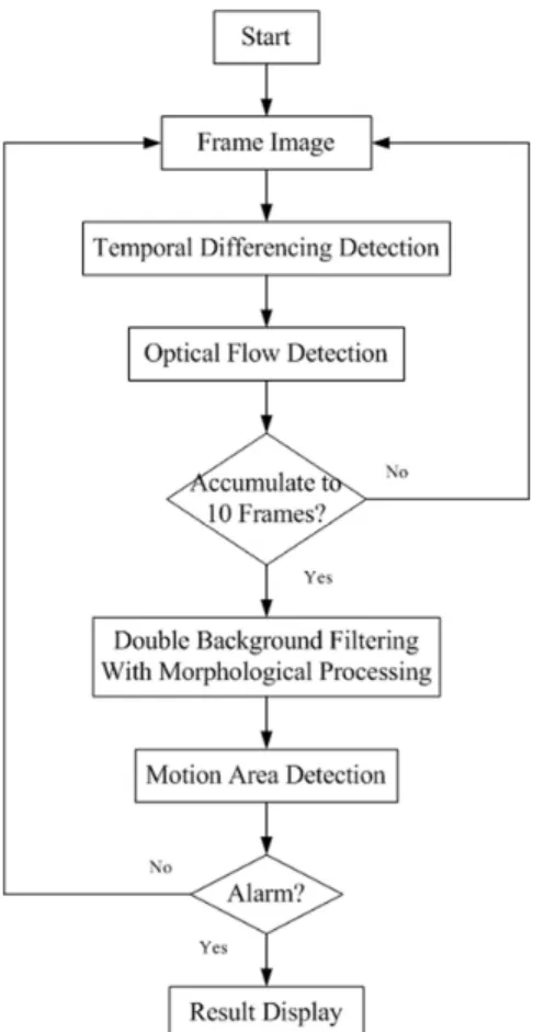
The method is depicted in the flow chart of Fig.1. As can be seen, the whole algorithm is comprised of four steps: (1) Temporal differencing method, which is used to detect the initial coarse object motion area; (2) Optical flow detection, which is based on the result of (1) to calculate optical flow for each frame; (3) Double background filtering method with morphological processing, which is used to eliminate the background interference and keep the foreground moving information; (4) Motion area detection, which is used to detect the moving object and give the alarming in time.
The final processing result is a binary image in which the background area and moving object area are shown as white color, the other areas are shown in black color and the top right corner is the alarm symbol. The experimental result in Section VI (Fig.5) presents a set of images to help in understanding the processes achieved in the present method.
Fig 1. Flowchart of motion detection method.
III. TEMPORAL DIFFERENCING DETECTION METHOD Temporal differencing is based on frame difference which attempts to detect moving regions by making use of the
difference of consecutive frames (two or three) in a video sequence. This method is highly adaptive to static environment. So temporal differencing is good at providing initial coarse motion areas.
In this paper, the two subsequent 256 level gray images at time t and t+1, I(x,y,t) and I(x,y,t+1), are selected and the difference between images is calculated by setting the adaptive threshold to get the region of changes. The adaptive threshold
d
T can be derived from image statistics. In order to detect cases of slow motion or temporally stopped objects, a weighted coefficient with a fixed weight for the new observation is used to compute the temporal difference image Id(x,y,t) as shown in following equations:
+ >
= +
otherwise T t y x I if t
y x
Id a d
0
) ) 1 , , ( ( 255 ) 1 , ,
( (1)
and
) , , ( ) 1 , , (
) , , ( ) 1 ( ) 1 , , (
t y x I t y x I w
t y x I w t
y x
Ia a
− + +
− = +
(2)
and
)) 1 , , ( (
3× +
= meanI x yt
Td a (3)
where w is a real number between 0 and 1 which describes the temporal range for difference images. Ia(x,y,t−1) is initialized to an empty image. In our method, we set Td as the
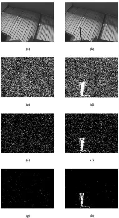
three times of mean value of Ia(x,y,t+1) and w=0.5 for all the results. Fig.2 below shows the results of temporal differencing method under a simulation environment which has a static background of our laboratory.
From the results, we can see that the temporal difference is a simple method for detecting moving objects in a static environment and the adaptive threshold Td can restrain the
noise very well. But if the background is not static, the temporal difference method will very sensitive to any movement and is difficult to differentiate the true and false movement. So the temporal difference method can only be used to detect the possible object moving area which is for the optical flow calculation to detect real object movement.
IV. OPTICAL FLOW DETECTION METHOD
Optical flow is a concept which is close to the motion of objects within a visual representation. The term optical flow denotes a vector field defined across the image plane. Optical flow calculation is a two-frame differential method for motion estimation. Such methods try to calculate the motion between two image frames which are taken at interval t at every pixel position. Estimating the optical flow is useful in pattern recognition, computer vision, and other image processing
applications [18]-[21]. In this chapter, a optical flow method entitled Lucas-Kanade Method is introduced.
Fig 2. Results of temporal differencing method. (a) Background image; (b) Background image with moving object; (c) Result of temporal difference for (a), Td=1×mean(Ia(x,y,t+1)); (d) Result of temporal differencing method for
(b), Td=1×mean(Ia(x,y,t+1)); (e) Result of temporal differencing method for
(a), T =2×mean(I (x,y,t+1))
a
d ; (f) Result of temporal differencing method for
(b), Td=2×mean(Ia(x,y,t+1)); (g) Result of temporal differencing method for
(a), Td=3×mean(Ia(x,y,t+1)); (h) Result of temporal differencing method for
(b), Td=3×mean(Ia(x,y,t+1)).
A. Lucas-Kanade Method
To extract a 2D motion field, Lucas-Kanade method is often employed to compute optical flow because of its accuracy and efficiency. Barron [22] compared the accuracy of different optical flow techniques on both real and synthetic image
sequences, it is found that the most reliable one was the first-order, local differential method of Lucas and Kanade. Liu [23] studied the accuracy and the efficiency trade-offs in different optical flow algorithms. The study has been focused on the motion algorithm implementation in real world tasks. Their results showed that Lucas Kanade method is pretty fast. Galvin [24] evaluated eight optical flow algorithms. The Lucas-Kanade method consistently produces accurate depth maps, and has a low computational cost, and good noise tolerance.
The Lucas-Kanade method [25] is trying to calculate the motion between two image frames which are taken at time t and t + δt for every pixel position. As a pixel at location (x,y,t) with intensity I (x,y,t) will have moved by δx, δy and δt between the two frames, the following image constraint equation can be given:
) , , ( ) , ,
(x yt I x x y yt t
I = +δ +δ +δ (4)
Assuming that the movement is small enough, the image constraint at I(x, y, t) with Taylor series can be derived to give:
T O H t t I y y I x x I
t y x I t t y y x x I
. . ) , , ( ) , , (
+ ∂ ∂ + ∂ ∂ + ∂ ∂ +
= + + +
δ δ δ
δ δ δ
(5)
where H.O.T. means those higher order terms, which are small enough to be ignored. From (4) and (5), the following can be obtained:
0 = ∂ ∂ + ∂ ∂ + ∂ ∂
t t I y y I x x
Iδ δ δ
(6)
or
0 = ∂ ∂ + ∂ ∂ + ∂ ∂
t t t I t y y I t x x I
δ δ δ δ δ δ
(7)
which will result in,
0 = ∂ ∂ + ∂ ∂ + ∂ ∂
t I V y I V x I
y
x (8)
where Vx and Vy are the x and y components of the velocity or
optical flow of I(x, y, t) and ∂I/∂x, ∂I/∂y and ∂I/∂t are the derivatives of the image at (x,y,t) in the corresponding directions.
Equation (8) is called the optical flow constraint equation since it expresses a constraint on the components Vx and Vy of
the optical flow. The optical flow constraint equation can be rewritten as:
t y y x
xV I V I
I + =− (9)
or
t y x y x I V V I
I =−
]
[ (10)
We wish to calculate Vx and Vy, but unfortunately the above
constraint gives us only one equation for two unknowns, so this is not enough by itself. To find the optical flow, another set of equations is needed which should be given by some additional constraints. The solution as given by Lucas and Kanade is a non-iterative method which assumes a locally constant flow.
The Lucas-Kanade algorithm assumed that motion vectors in any a given region do not change but merely shift from one position to another. Assuming that the flow (Vx, Vy) is a
constant in a small window of size
m
×
m
with m > 1, which is centered at (x, y) and numbering the pixels as 1...n, a set of equations can be derived:n n
n x y y t
x t y y x x t y y x x I V I V I I V I V I I V I V I − = + − = + − = + M 2 2 2 1 1 1 (11)
With (11), there are more than three equations for the three unknowns and thus the system is over-determined. Hence:
− − − = n n n t t t y x y x y x y x I I I V V I I I I I I M M M 2 1 2 2 1 1 (12) or b v
Ar=− (13) To solve the over-determined system of equations, the least squares method is used:
) ( b A v A
AT r= T −
(14)
) ( )
(A A 1A b
vr= T − T − (15) or − − =
∑
∑
∑
∑
∑
∑
− i i i i i i i i i i t y t x y y x y x x y x I I I I I I I I I I V V 1 2 2 (16)with the sums running from i=1 to n. And there is a limit condition for the calculation of motion vector in (16) as:
=
∑
∑
∑
∑
2 2 i i i i i i y y x y x x T I I I I I I AA (17)
Equation (17) must be an invertible matrix, which means that the optical flow can be found by calculating the derivatives of the image in all three dimensions: x-direction, y-direction and
t-direction. One of the characteristics of the Lucas-Kanade algorithm is that it does not yield a very high density of flow vectors, i.e. the flow information fades out quickly across motion boundaries and the inner parts of large homogenous areas show little motion. The advantage for the method is its accuracy and robustness of detection in presence of noise.
B. Simplified Calculation
The theoretical calculation procedure of the optical flow method is explained in the above subsection, but for the requirement of practical application, some operation characteristics between matrices can be used to simplify the complexity of calculation. For the calculation of invertible matrix in (16), the companion matrix method can be used:
− − = = ∗ − ] 0 ][ 0 [ ] 1 ][ 0 [ ] 0 ][ 1 [ ] 1 ][ 1 [ det 1 1 M M M M M M M
M (18)
where M* is the companion matrix of M and M is the determinant of M.
C. Gradient Operator
From the operation expression of optical flow, the estimation of the gradient for x-direction, y-direction and t-direction, has a great influence on the final results of optical flow calculation. The most common gradient operators used in optical flow calculation are Horn, Robert, Sobel, Prewitt, Barron and so on. In this paper, a better 3D Sobel operator is used which was proposed in [26]. This operator uses three different templates to do the convolution calculation for three frames in a row along the directions of x, y and t and to calculate the gradient along three directions for central pixels of the template in the middle frame. Fig.3 shows the operators.
Fig 3. 3D Sobel operator for optical flow calculation.
D. Results of Optical Flow Detection
The optical flow information for every frame of an image is calculated. As shown in Fig.4, the optical flow of frames
n t t
t I I
I, +1,K, + in a period time [t, t+n] are represented as
n
F F
F1, 2,K, (here i represent i sampling period in t+i expression). The result of optical flow is shown as a binary image and the adaptive threshold is selected to distinguish the moving pixel from the still pixel. The pixels whose optical flow values are greater than threshold will be considered as moving pixels and are shown in white.
Fig 4. Diagram of optical flow calculation.
The optical flow value and the adaptive threshold formulas that we used can be written as:
) , ( ) , ( ) ,
(i j V2 i j V2 i j
Fn = x + y (19)
and
>
=
Otherwise T j i F if j
i
FDn n
0
) , ( 255
) ,
( (20)
and
) 0 ) , (
( >
=median F i j
T n (21)
where Fn(i,j) is the optical flow value, FnD(i,j)is the result
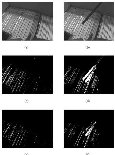
of optical flow detection and the adaptive threshold T is select as median value of Fn(i,j)whose value is above 0. Fig.5 shows the results of optical flow which is calculated based on the result of temporal difference. The simulation environment this time is not a static background which the column bar curtain is moving caused by the winds.
From the results, we can see that the optical flow with adaptive threshold based on temporal difference reserves the information of moving object very well. However, because of the background interference of the image, the real object movement still can not be separated from the background. So the method of double background filtering with morphological processing is introduced in the next section to deal with this problem.
V. DOUBLE BACKGROUND FILTERING WITH MORPHOLOGICAL PROCESSING
By using the optical flow method, two types of optical flow information are obtained, which are the interference information of image background and the information of image pixel with any possibility of real object movement. In the real situation, because of the environment such as light, vibration and so on, the interference information of the background still
can be detected. Sometimes, it is difficult for the real object movement to be differentiated from the background interference. In this section, the method of DBF with morphological processing is used to get rid of the background interference and separate the moving object from it. Firstly, the DBF method and its corresponding results are discussed. Then the morphological processing methods are introduced and the improved results are also demonstrated.
Fig 5. Results of optical flow based on temporal difference method. (a) Background image; (b) Background image with moving object; (c) Result of temporal difference for (a); (d) Result of temporal difference for (b); (e) Result of optical flow for (c); (f) Result of optical flow for (d).
A. Double Background Filtering
In this paper, a novel approach is developed to update the background. This approach is based on a double background principle [27]-[28], long-term background and short-term background. For the long-term background, the background interference information which has happened in a long time is saved. For the short-term background, the most recent changes are saved. These two background images are modified to adequately update the background image and to detect and correct abnormal conditions.
During practical tests, we found that although the optical flow of background interference can be detected without moving object, it is relatively stable for some specific areas on the image and the amount of this optical flow doesn’t change
very much. For the area where the moving object appears, the amount of optical flow must change significantly in the specific area. According to these characteristics, the moving object should be easily detected if the information of the background and foreground can be separated. In this paper, a method entitled Double Background Filtering (DBF) is proposed, which consists of four steps. Fig.6 shown below explains the method in a tabular way.
Fig 6. The double background filtering method.
1) The optical flow information of the first five frames is accumulated for saving the optical flow information of the background interference. Let 5
A be the accumulation matrix, which is defined with the same size as the video images and set the initial value as zeros. To compute this matrix the formula below is applied:
5 , 4 , 3 , 2 , 1 0 ) , ( ) , (
255 ) , ( 1 ) , ( ) ,
( 5
5
5 =
= = +
= k
j i F if j i A
j i F if j i A j i A
k k
(22)
2) The optical flow information of the last three frames is accumulated for moving object detection. Let 3
A be the accumulation matrix and computed as follow:
10 , 9 , 8 0
) , ( )
, (
255 ) , ( 1 ) , ( ) ,
( 3
3
3 =
= = +
= k
j i F if j i A
j i F if j i A j i A
k k
(23)
3) By comparing the results of steps (1) and (2) and eliminating the overlap optical flow, the rest should be the optical flow which represents as the real movement. The algorithm to detect whether a pixel B(i, j) belongs to an object with salient motion is described as follows:
> =
> >
=
0 ) , ( 0
) , ( 255
0 ) , ( 0
) , ( 0
) ,
( 5 3
3 5
j i A and j
i A if
j i A and j
i A if j
i
B (24)
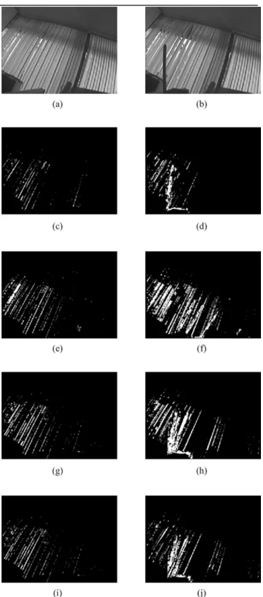
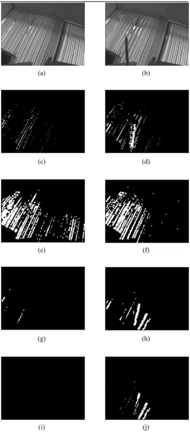
Fig 7. Results of double background filtering method. (a) Background image; (b) Background image with moving object; (c) Result of optical flow for (a); (d) Result of optical flow for (b); (e) Result of first five frames optical flow accumulation for (c); (f) Result of first five frames optical flow accumulation for (d); (g) Result of last three frames optical flow accumulation for (c); (h) Result of last three frames optical flow accumulation for (d); (i) Result of double background filtering for (c); (j) Result of double background filtering for (d);
4) Background Updating, This step is an updating function of the new value of the accumulation matrix, both 5
A and
3
A are set to zero, with the new video frame input, the four steps above are then repeated.
In this method, there are always two unused frames during the process, the purpose of this is to separate the background and moving object effectively. When the moving object appears in the last three frames, the information of moving object will not be lost while the background is updating. Fig.7 shows the result of double background filtering method.
From the results, we can see that for the background without moving object, the background interference can not be eliminated completely and for the background with moving object, although the moving object area can be detected, the background interference is still exit. So how to get rid of the background interference and preserve the information of moving object at the same time is most important problem we are facing. The morphological processing method is introduced in next section to solve this problem.
B. Morphological Image Processing
Morphological image processing is a collection of techniques for digital image processing based on mathematical morphology which is a nonlinear approach that is developed based on set theory and geometry [29]. Morphological image processing techniques are widely used in the area of image processing, machine vision and pattern recognition due to its robustness in preserving the main shape while suppressing noise. When acting upon complex shapes, morphological operations are able to decompose them into meaningful parts and separate them from the background, as well as preserve the main shape characteristics. Furthermore, the mathematical calculation involved in mathematical morphology includes only addition, subtraction and maximum and minimum operations without any multiplication and division. There are two fundamental morphological operations which are dilation and erosion and many of the morphological algorithms are based on these two primitive operations.
Dilation of the set A by set B which is usually called as structure element, denoted by A⊕B , is obtained by first reflecting B about its origin and then translating the result by x. All x such that A and reflected B translated by x that have at least one point in common form the dilated set.
} )
ˆ ( |
{ ∩ ≠∅
=
⊕B x B A
A x (25)
where Bˆ denotes the reflection of B and (B)xdenotes the
translation of B by x. Thus, dilation of A by B expands the boundary of A.
Erosion of A by B, denoted byAΟB, is the set of all x such that B translated by x is completely contained in A.
Fig 8. Results of double background filtering method. (a) Background image; (b) Background image with moving object; (c) Result of optical flow for (a); (d) Result of optical flow for (b); (e) Result of first five frames optical flow accumulation after dilation for (c); (f) Result of first five frames optical flow accumulation after dilation for (d); (g) Result of last three frames optical flow accumulation after opening and closing for (c); (h) Result of last three frames optical flow accumulation after opening and closing for (d); (i) Result of double background filtering with morphological processing for (c); (j) Result of double background filtering with morphological processing for (d);
} ) ( |
{x B A
B
AΟ = x⊆ (26)
Thus, erosion of A by B shrinks the boundary of A. In this paper we also use two other important morphological operations which are defined in terms of erosion and dilation: opening and closing.
A is said to be opened by B if the erosion of A by B is followed by a dilation of the result by B.
B B A B
Ao =( Ο )⊕ (27) Opening generally smoothes the contour of an object, breaks narrow isthmuses, and eliminates thin protrusions.
Similarly, A is said to be closed by B if A is first dilated by B
and the result is then eroded by B. Thus,
B B A B
A• =( ⊕ )Ο (28) Closing also tends to smooth sections of contours but, as opposed to opening, it generally fuses narrow breaks and long thin gulfs, eliminates small holes, and fills gaps in the contour. In our experiments, we use three morphological operators, dilation, opening and closing. The first one, dilation, is applied in the image with the accumulation optical flow for the first five frames, which is after the first step of DBF method. The dilation operator expands the area of background interference to make it eliminated efficiently in the third step of DBF method. The other two operators, opening and closing, are applied in the image with the accumulation optical flow for last three frames, which is after second step of DBF method. The opening operator is used first to eliminate the noise which consists of isolated points and closing operator is used immediately after filling up the holes and gaps. The structure element in both operations isSE={1,1,1;1,1,1;1,1,1}. Fig.8 shows the results of DBF with morphological processing.
From the results, we can see that the DBF method with morphological processing can preserve the moving object area very well and eliminate the background interference completely. The result of this processing can be very helpful for the further motion area detection.
VI. MOTION AREA DETECTION
After applying the step of DBF method with morphological processing, the optical flow information of the background interference should be eliminated and only the optical flow information of real moving object is left. During the experimental test, we find that the appearance of a moving object can make a big influence on the instantaneous rate of change between the foreground motion information and the accumulative background optical flow information. In this paper, we use the result of DBF method with morphological processing as the foreground motion information FM. Because the result of DBF method with morphological processing comes from the last three frames accumulative optical flow
information so that the result of the first seven frames accumulative optical flow information is used as the accumulative background optical flow information ABOF7. So
we can define the instantaneous rate of change for the moving object appearance IRCA as follows:
% 100 7
× =
ABOF FM
IRCA (29)
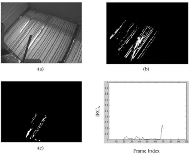
Fig.9 and Fig.10 show the result of IRCA during the experiments for the background with and without moving object, respectively.
Fig 9. Results of IRCA for the background without moving object. (a) Background image; (b) Result of optical flow; (c) Result of DBF method; (d) Result of IRCA.
Fig 10. Results of IRCA for the background with moving object. (a) Background image; (b) Result of optical flow; (c) Result of DBF method; (d) Result of IRCA.
From the results, we can see that, for the background without moving object, IRCA has a small value with little changing. But if there is moving object appearance, the value of IRCA will increase sharply and last for several frames time. By taking advantage of this feature, we can use this IRCA value to detect the movement of moving object and give the alarm without delay. In our experiment, the alarm threshold T is set as 0.25 and the abnormity alarm will occur whenever the IRCA value is above T. It can be described as follows:
>
=
Otherwise T IRC if
A A
0 1
(30)
where A is the symbol for alarming, 0 and 1 represent whether the alarm is on.
VII. CONCLUSION
The algorithm is implemented in Matlab program. The size of the input video image is 320×240 pixels and the sample rate is 25 frames per second. In this experiment, the simulation environment is the background of a column strip curtain which is swing caused by nature winds.
In this paper a new approach is proposed for motion detection using temporal differencing method, optical flow method, double background filtering method and morphological processing methods. The paper integrates the advantages of these all methods and presents a fast and robust motion detection algorithm. The paper introduces the temporal differencing method first to detect the initial coarse motion object area. Then the optical flow method is applied based on the result of temporal differencing method to calculate any possible movement pixel for each video frame. Because of the temporal differencing method, the calculation demand for the optical flow is reduced greatly and the moving area is still detected accurately. Then, the paper presents an improved motion detection algorithm based on a double background filtering technique with morphological processing. The DBF method is used to obtain and keep a stable background image to cope with the appearance of the moving object and is used to eliminate the background interference and separate the foreground moving object from it. The morphological processing methods are used and combined with DBF to gain the better results. Finally, the calculation of the instantaneous rate of change for the moving object appearance is used for the motion detection. The experiments indicated that the algorithm can detect moving objects precisely, including slow moving or tiny objects, and give an alarm in time.
ACKNOWLEDGEMENT
The authors would like to thank BlueStar Technology Co., Ltd., for their financial and equipment supports. The authors also wish to thank Mr. CaiGuang He and Mr. XiaoHui Gao for their helpful advices for this work.
REFERENCES
[1] Y.L. Tian and A. Hampapur, “Robust Salient Motion Detection with Complex Background for Real-time Video Surveillance,” IEEE Computer Society Workshop on Motion and Video Computing, Breckenridge, Colorado, January 5 and 6, 2005.
[2] C. Bahlmann, Y. Zhu, Y. Ramesh, M. Pellkofer, T. Koehler, “A system for traffic sign detection, tracking, and recognition using color, shape, and motion information,” IEEE Intelligent Vehicles Symposium, Proceedings,2005,pp. 255-260.
[3] A. Manzanera and J.C. Richefeu, “A new motion detection algorithm based on Σ-∆ background estimation,” Pattern Recognition Letters, vol. 28, n 3, Feb 1, 2007, pp. 320-328.
[4] Y, Ren, C.S. Chua and Y.K. Ho, “Motion detection with nonstationary background,” Machine Vision and Applications, vol. 13, n 5-6, March, 2003, pp. 332-343.
[5] J. Guo, D. Rajan and E.S. Chng, “Motion detection with adaptive background and dynamic thresholds,” 2005 Fifth International Conference onInformation, Communications and Signal Processing, 06-09 Dec. 2005, pp. 41-45.
[6] A. Elnagar and A. Basu, “Motion detection using background constraints,” Pattern Recognition, vol. 28, n 10, Oct, 1995, pp. 1537-1554.
[7] J.F. Vazquez, M. Mazo, J.L. Lazaro, C.A. Luna, J. Urefla, J.J. Garcia and E. Guillan, “Adaptive threshold for motion detection in outdoor environment using computer vision,” Proceedings of the IEEE International Symposium onIndustrial Electronics, 2005. ISIE 2005, vol. 3, 20-23 June 2005, pp. 1233-1237.
[8] P. Spagnolo, T. D'Orazio, M. Leo and A. Distante, “Advances in background updating and shadow removing for motion detection algorithms,” Lecture Notes in Computer Science, vol. 3691 LNCS, 2005, pp. 398-406.
[9] D.E. Butler, V.M. Bove Jr. and S. Sridharan, “Real-time adaptive foreground/background segmentation,” Eurasip Journal on Applied Signal Processing, vol. 2005, n 14, Aug 11, 2005, pp. 2292-2304. [10] Y.S. Choi, Z.J. Piao, S.W. Kim, T.H. Kim and C.B. Park, “Salient
motion information detection technique using weighted subtraction image and motion vector,” Proceedings of 2006 International Conference on Hybrid Information Technology, vol. 1, 2006, pp. 263-269.
[11] J.W. Wu and M. Trivedi, “Performance characterization for gaussian mixture model based motion detection algorithms,” Proceedings of International Conference on Image Processing, vol. 1, 2005, pp. 1097-1100.
[12] P.R.R. Hasanzadeh, A. Shahmirzaie and A.H. Rezaie, “Motion detection using differential histogram equalization,” Proceedings of the Fifth IEEE International Symposium on Signal Processing and Information Technology, 2005, pp. 186-190.
[13] D.X. Zhou and H. Zhang, “Modified GMM background modeling and optical flow for detection of moving objects,” Conference Proceedings of IEEE International Conference on Systems, Man and Cybernetics, vol. 3, 2005, pp. 2224-2229.
[14] G. Jing, C.E. Siong and D. Rajan, “Foreground motion detection by difference-based spatial temporal entropy image,” IEEE Region 10 Conference Proceedings: Analog and Digital Techniques in Electrical Engineering, 2004, pp. 379-382.
[15] C.C. Chang, T.L. Chia and C.K. Yang, “Modified temporal difference method for change detection,” Optical Engineering, vol. 44, n 2, February, 2005.
[16] Y. Shan and R.S. Wang, “Improved algorithms for motion detection and tracking,” Optical Engineering, vol. 45, n 6, June 2006.
[17] N. Lu, J.H. Wang, Q.H. Wu and L. Yang, “Motion detection based on accumulative optical flow and double background filtering,” Proceedings of World Congress on Engineering, London, UK, 2-4 July, 2007, pp. 602-607.
[18] J. Lin, J.H. Xu, W. Cong, L.L. Zhou and H. Yu, “Research on real-time detection of moving target using gradient optical flow,” IEEE International Conference on Mechatronics and Automation, 2005, pp. 1796-1801.
[19] E. Trucco, T. Tommasini and V, Roberto, “Near-recursive optical flow from weighted image differences,” IEEE Transactions on Systems, Man, and Cybernetics, Part B: Cybernetics, vol. 35, n 1, February, 2005, pp. 124-129.
[20] H. Ishiyama, T. Okatani and K. Dequchi, “High-speed and high-precision optical flow detection for real-time motion segmentation, ” Proceedings of the SICE Annual Conference, 2004, pp. 751-754.
[21] L. Wixson, “Detecting salient motion by accumulating directionally-consistent flow,” IEEE Transactions onPattern Analysis and Machine Intelligence, vol. 22, issue 8, Aug. 2000, pp. 774-780. [22] J. Barron, D. Fleet and S. Beauchemin, “Performance of Optical Flow
Techniques,” International Journal of Computer Vision, vol. 12, n 1, 1994, pp. 42–77.
[23] H. Liu, T. Hong, M. Herman and R. Chellappa, “Accuracy vs. Efficiency Trade-offs in Optical Flow Algorithms,” In the Proceeding of Europe Conference Of Computer Vision, 1996.
[24] B. Galvin, B. McCane, K. Novins, D. Mason, and S.Mills, “Recovering Motion Fields: An Evaluation of Eight Optical Flow Algorithms,” In Proc. Of the 9th British Machine Vision Conference (BMVC’98), vol. 1, Sep. 1998, pp. 195-204.
[25] Wikipedia, the free encyclopedia. 20 February 2007. Lucas Kanade method. Available: http://en.wikipedia.org/wiki/Lucas_Kanade_method [26] J. Lopez, M. Markel, N. Siddiqi, G. Gebert and J. Evers, “Performance
of passive ranging from image flow,”IEEE International Conference on Image Processing, vol. 1, 2003, pp. 929-932.
[27] H.J. Elias, O.U. Carlos and S. Jesus, “Detected motion classification with a double-background and a neighborhood-based difference,” Pattern Recognition Letters, vol. 24, n 12, August, 2003, pp. 2079-2092.
[28] J. Zheng, B. Li, B. Zhou and W. Li, “Fast motion detection based on accumulative optical flow and double background model,” Lecture Notes in Computer Science, Computational Intelligence and Security - International Conference, CIS 2005, Proceedings, vol. 3802 LNAI, 2005, pp. 291-296.
[29] R.C. Gonzalez and R.E. Woods, Digital Image Processing, Prentice-Hall, December, 2002, Second edition, ISBN: 0130946508.