Controlling nonholonomic Chaplygin systems
Antonio Carlos Baptista Antunes∗ and C´assio Sigaud†
Deptamento F´ısica Matem´atica, Instituto de F´ısica, Universidade Federal do Rio de Janeiro, Caixa Postal 68.528, 21.941-972 Rio de Janeiro RJ, Brasil
Pedro Claudio Guaranho de Moraes‡
Departamento de Engenharia de Biossistemas, Universidade Federal de S˜ao Jo˜ao del-Rei, 36.301-160 S˜ao Jo˜ao del-Rei MG, Brasil (Received on 6 April, 2009)
In this paper we deal with the problem of controlling some Chaplygin systems in the framework of the vakonomic approach for nonholonomic systems. Equations of motion for these systems are obtained which contain a free parameter that permits to control the system. It is show that given a prescribed path it is possible to determine the parameter of control which inserted in the equations of motion compel the trajectory of the system to follow the input function.
Keywords: Nonholonomic systems; vakonomic approach; Chaplygin systems.
1. INTRODUCTION
The subject of nonholonomic systems has a long history since the observation by Hertz that some types of mechan-ical systems subjected to nonintegrable constraints cannot be analysed in the framework of the lagrangian mechanics [1]. This means that the lagrangian formulation of mechan-ics does not give the correct equations of motion for these systems. The problem introduced by the so called nonholo-nomic constraints was circunvented by the introduction of the method of the lagrangian multipliers in lagrangian me-chanics [2–4]. Since that times, nonholonomic systems are analysed on the basis of the Lagrange-d’Alambert principle and some others equivalent approaches [5].
More recently, it was observed that the nonholonomic con-traints are an open window to the possibility of controlling nonholonomic systems. The Lagrange multiplier method conjugated with an adequate variational procedure gives a set of equations of motion which contain free parameters that can be used to compel the system to follow a prescribed path. This formulation, the so called variational axiomatic kind for nonholonomic systems or shortly vakonomic approach for nonholonomic system [6], is the procedure used in this paper to obtain the equations of motion of an instructive example, the Chaplygin sleigh [7], which is very convenient to shed some light on the details of the controlling mechanisms.
The general problem of the nonholonomic scleronomous systems consists in given a lagrangianL(q,q)˙ and a set of constraint equations,
n
∑
j=1
al j(q)q˙j=0 (ℓ=1, ...,m<n), (1)
to seek for the correct equations that describe the au-tonomous motion of the system, can be approached by the Lagrange-d’Alembert principle.
On the other hand, if we intend to obtain the equations of motion for a prescritive mechanics which admits the
possi-∗Electronic address:[email protected]
†Electronic address:[email protected] ‡Electronic address:[email protected]
bility of controlling the system, according to the vakonomic approach, the lagrangian must be extended to include the nonholonomic constraint conditions,
L′=L(q,q) +˙ m
∑
ℓ=1
λℓ n
∑
j=1
aℓj(q)q˙j, (2)
whereλℓ(ℓ=1, ...,m)are the Lagrange multipliers. The Hamiltonian principle,
δ
Z
L′dt=0, (3)
whereL′is the constrained lagrangian, gives the equations of the motion,
∂L′
∂qj− d dt
∂L′
∂q˙j
=0, (j=1, ...,n), (4) which are explicitly,
∂L
∂qj− d dt
∂L
∂q˙j− m
∑
ℓ=1 ˙
λℓaℓj+ m
∑
ℓ=1
λℓ n
∑
k=1
∂aℓk
∂qj −
∂aℓj
∂qk
˙
qk=0, (j=1, ...,n), (5) together with the constraint equations,
n
∑
j=1
aℓj(q)q˙j=0, (ℓ=1, ...,m). (6)
Using thesen+mequations, it is possible to determine the ˙
λℓ(ℓ=1, ...,m), which are the forces of the constraints on the system. The remainingλℓare free parameters which can be conveniently chosen in order to force the system to follow a prescribed path in the coordinate space.
Our aim is to use a simple model, the Chaplygin sleigh to enlighten the procedure of determining the free parameters of controlλℓ, which drive the system along a chosen curve given by a function on the horizontal plane.
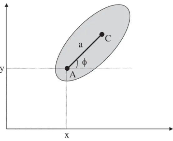
2. THE MODEL
a C
y
x A
f
FIG. 1: The Chaplygin sleigh.
sleigh. This apparatus consists of an eliptical board moving on a horizontal plane supported by two sliding points and a knife edge rigidly fixed under the board along the longitudi-nal axis. The contact point of the knife with the horizontal plane is at a distanceaof the center of mass of the system. The coordinates used to describe the motion of this system are(x,y), the coordinates of the point of contact of the knife with the plane,φthe angle between the knife (and the longi-tudinal axis of the board) and thexaxis on the plane.
Let ˙sbe the velocity of the point of contact of the knife. Its cartesian components are,
˙
x=s˙cos(φ) and ˙y=˙s sin(φ). (7) The equation for the constraint condition on the system is,
−x˙sin(φ) +y˙cos(φ) =0. (8) Letmbe the mass of the sleigh andIthe moment of iner-tia of the board and the knife around a vertical axis passing through the center of mass. The kinetic energy of the system is,
T=1 2m x˙
2+ ˙ y2+1
2 I+ma 2φ˙2+
maφ˙(−x˙sin(φ) +y˙cos(φ)). (9) Following the vakonomic prescriptions described above, we write the extended lagrangian,
L′=T+λ(−x˙sin(φ) +y˙cos(φ)), (10) or
L′=1 2m x˙
2+ ˙
y2+b2φ˙2+
λc φ˙
(−x˙sin(φ) +y˙cos(φ)), (11) where,
b= r
a2+ I
m, (12)
is the radius of gyration of the system and
λc φ˙
= λ+maφ˙. (13)
The equations (4) are used to obtain the equations of motion of the Chaplygin sleigh. In this way, we obtain the equations of the motion of the system,
¨
x=−sin(φ) (x˙cos(φ) +y˙sin(φ))φ˙+λc
mcos(φ)φ˙, (14) ¨
y=cos(φ) (x˙cos(φ) +y˙sin(φ))φ˙+λc
msin(φ)φ˙, (15) ¨
φ=−
λc mb2
(x˙cos(φ) +y˙sin(φ)). (16) Together with the equation that gives the force of the con-straint,
˙
λc=−m(x˙cos(φ) +y˙sin(φ))φ˙. (17) Using the constraint equation 8 and the velocity of the knife contact point,
˙
s=x˙cos(φ) +y˙sin(φ), (18) the set of equations above can be written more compactly as,
¨ s = λc
mφ˙, (19)
¨
φ = −mbλc2s˙, (20)
and
˙
λc=−ms˙φ˙. (21)
A more convenient set of variables is,
u1 = √ms˙, (22)
u2 =
√
mbφ˙, (23)
and
Λ=χ˙+a
bφ˙, (24)
where
˙
χ= λ
mb. (25)
In terms of these variables, the set of equations above reads,
˙
u1 = Λu2, (26)
˙
u2 = −Λu1, (27)
and
˙
Λ=−mb12u1u2. (28)
Besides these equations, we have the dynamical condition,
u21+u22=2T, (29) which comes from the expression for the kinetic energy. The relations (26), (27) and (29) suggest that the variablesu1and u2can be written in sinusoidal forms:
u1 = √2Tsin(Ψ), (30) u2 =
√
whereΨis an angle that can easily be related to the param-eterΛ. Putting the functions (30) and (31) in the equations (26) and (27), we obtain,
˙
Ψ=Λ, (32)
then,
Ψ=χ+a
bφ. (33)
In terms of the configuration coordinates the above equa-tions read:
˙
s = vTsin(Ψ), (34)
˙
φ = vT
b cos(Ψ), (35)
and
˙
x = vTsin(Ψ)cos(φ), (36) ˙
y = vTsin(Ψ)sin(φ), (37) where,
vT= r
2T
m. (38)
This set of equations is usually obtained in the framework of the differential geometric formulation of nonholonomic mechanics [8] andu1=
√
2Tsin(Ψ)andu2=
√
2Tcos(Ψ) are called the controls of the system. Using a matrix notation and definingu= (u1,u2)⊤the set of equations (26), (27) and (32) can be integrated giving,
u(t) =eΨ(t)Juo, (39) where J is the simpletic matrix,
J=
0 1
−1 0
. (40)
3. THE AUTONOMOUS MOTION
Choosing χ=0, the equations of motion (36) and (37) become,
˙
x = vTsin(Ψ)cos
b aΨ
, (41)
˙
y = vTsin(Ψ)sin
b aΨ
. (42)
These are the same equations obtained by Neimark and Fu-faev [5] for the motion of the Chaplygin sleigh in the hori-zontal plane and free from external forces and torques.
4. THE CONTROLLED MOTION
The angleΨis related to the components of the center of mass velocity. Using the equations (34), (35) and the defini-tions ofu1andu2, we obtain,
tanΨ=
˙ s bφ˙
, (43)
Where ˙sis the component of the center of mass velocity in the direction of the longitudinal axis of the sleigh ( and of the knife ) andbφ˙is the transversal component. We introduce the variable,
ρ= s˙ ˙
φ, (44)
where,|ρ|is the radius of curvature of the trajectory. Then the above equation reads,
tan(Ψ) =ρ
b. (45)
The equation (45) is of fundamental importance in the pro-cess of controlling the system. It is this equation that deter-mines the control parameterΨ, for a prescribed path imposed to the system.
In order to clarify this detail of the controlling procedure we consider the problem of to compel the Chaplygin sleigh to follow a path described by a well behaved functiony=y(x) in the plane (x,y) with finite derivatives y′(x) =tanφ and y′′(x). The radius of curvature of this path is given by,
ρ(x) =
1+y′(x)232
y′′(x) . (46)
Then, the angle of controlΨis obtained from,
tanΨ=
1+y′(x)232
by′′(x) . (47)
Under the above conditions we have tan(Ψ)∈(−∞,∞)and
Ψ∈(−2π,π2).
For a parametric curvex(s),y(s)the equation (45) gives,
tanΨ= 1
b[x′(s)y′′(s)−y′(s)x′′(s)]. (48) This kind of procedure by which the equations of motion of the system are determined such that the trajectory of the system follows on the prescribed path is the first stage of the control process sometimes called planning or tracking [9].
An immediate application of these results is the compu-tation of the time of the motion along the given trajectory between two pointss=0 ands(t).
The kinetic energy of the system is,
T=m 2
h ˙
s2+ bφ˙2i, (49) and can be rewritten as,
vT = ˙ s
sin(Ψ). (50)
Then, the time of the motion is given by:
t= 1 vT
s(t)
Z
0 ds
sin(Ψ). (51)
For a given input functionx(s),y(s), sin(Ψ) =p ρ(s)
and the time expended along the motion is given by
t= 1 vT
s(t)
Z
0 p
b2+ρ2(s)
ρ(s) ds. (53)
5. THE CONTROL SYSTEM
In order to examine the physical aspects of the control pro-cess, we return to the constrained Lagrangian,
L′=1 2m x˙
2+ ˙ y2+1
2mb 2φ˙2+
λ+maφ˙(−x˙sinφ +y˙cosφ). (54) The angular momentum of the system
pφ=
∂L′
∂φ˙ =mb
2φ˙,
(55)
is not a conserved quantity because there is a torque:
ℑφ=∂
L′
∂φ =− λ+maφ˙
(x˙cosφ +y˙sinφ), (56) or
ℑφ=− λ+maφ˙s˙. (57)
This torque changes the angular momentum of the Chap-lygin sleigh around the contact point of the knife which is shown by the equation of motion
mb2φ¨=−λs˙−mas˙ 2
ρ. (58)
This first term(−λs)˙ is due to an external system which con-trols the motion of the Chaplygin sleigh. The second term is a torque due to the centrifugal force that appears in the accelerated frame fixed in the Chaplygin sleigh.
However, the formulation above requires that the kinetic energy
T =1 2 u
2 1+u22
(59)
must be a constant along the controlled motion. The equa-tions (26) and (27) give,
dT
dt =u1u˙1+u2u˙2=0. (60) It is easy to see that if the system is under the action of a torque solely, the energy is not conserved. The kinetic energy is,
T =m 2 v
2 c+Iφ˙2
, (61)
where,
− →v
c =s˙bs+aφ˙bφ, (62)
then,
dT dt =m
− →v
c·−→v˙c+Iφ˙φ¨
. (63)
However,m−→v˙c=F→−c andIφ¨=ℑc, which are a force applied on the center of mass and a torque, respectively.
Using these relations, we obtain:
dT dt =
−
→vc·→−Fc+φℑ˙ c. (64)
If−→Fc=0 andℑc6=0 then dTdt 6=0.
In order to obtain a control system that does not change the kinetic energy, we must impose ˙sFcs+ aFcφ+ℑc
˙
φ=0. Using ˙s=ρφ˙, we obtain,
Fcs=− 1
ρ aFcφ+ℑc
. (65)
In the absence of a torque,ℑc=0, the condition for energy conservation is
− →v
c·−→Fc=0, (66) then,−→Fc⊥ −→vc and,
Fcs=− a
ρFcφ. (67)
Introducing the following notation,
−
→rc =−→ccc=−ρbφ+abs, (68)
whereccis the center of the curvature of the path, we obtain
−
→rc· −→vc=0,then−→Fc k −→rc, and the force−→Fc is applied incin the direction ofcc.
In order to determine the force that must be applied on the CM for the system to follow a given path, we use the relations,
Fcφ=m aφ¨+ρφ˙2, (69)
and
¨
φ=−ρbφ˙ψ˙, then
Fcφ=mρφ˙
−abψ˙+φ˙, (70) where
˙
ψ=χ˙+a
6. EXAMPLES OF TRACKING
The first example is the motion along a straigh line given by,
y(x) =Ax+B. (72)
The angles of this trajectory are:
φ=arctan(A), (73)
tan(Ψ) =ρ
b =∞, (74)
then,
Ψ=π
2, (75)
and
χ=π
2− a
barctan(A), (76)
which are all constants. The scalar velocity is,
˙
s=vTsin(Ψ) =vT, (77) and the equations of motion are,
˙
x = vTcos(φ), (78)
˙
y = vTsin(φ). (79)
The equations of the trajectory are,
x(t) = √ vT
1+A2t, (80)
y(t) = √AvT
1+A2t+B. (81)
A second example is the case of a circular trajectory with radiusR,
x=Rcos s
R
, y=Rsin
s R
. (82)
Then
x′y′′−y′x′′= 1
R, (83)
and the equation (45) gives,
tan(Ψ) =R
b, (84)
which is a constant.
The period of circulation is
tc= 1 vT
I √b2+R2
R ds=π r
2m T
p
b2+R2. (85) Besides the angleΨwe have
tan(φ) =y′(s)
x′(s)=−cot s
R
, (86)
then,
φ= s
R+
π
2. (87)
The angleχ which is the parameter that drives the system along the circular path is,
χ(s) =arctan
R b
−abRs +π 2
. (88)
The time evolution is given by,
˙
s=vTsin(Ψ) = vTR
√
b2+R2, (89)
then,
s(t) =√vTR
b2+R2t. (90)
The cartesian coordinates of the trajectory are given by,
˙
x = √vTR
b2+R2cos
π
2+ vT
√
b2+R2t
, (91)
˙
y = √vTR
b2+R2sin
π
2+ vT
√
b2+R2t
. (92)
Then,
x(t) = Rcos
vT
√
b2+R2t
, (93)
y(t) = Rsin
vT
√
b2+R2t
, (94)
and
˙
φ = s˙
R= vT
√
b2+R2 (95)
is the angular velocity of the system along the circular tra-jectory. The time dependence of the driving angle is,
χ(t) =arctan
R b
−ab
π
2+ vT
√
b2+R2t
. (96)
The third example consists of an input path given by the parametric equations of a catenary,
x(s) = q
s2+x2
o, (97)
y(s) =xoln
s+ q
s2+x2 o
, (98)
wheres≥0 is the arc lengh of the path. The radius of curvature is,
ρ(s) = s
2+x2 o
xo
, (99)
and the angle of control along this path is given by,
tan(Ψ) =ρ b =
s2+x2o b xo
0 5 10 15 20 25 30 0
5 10 15 20 25 30
0 5 10 15 20 25 30
0 5 10 15 20 25 30
0 5 10 15 20 25 30
0 1 2 3 4
0 5 10 15 20 25 30
0 1 2 3 4 S
a
X
y y
t
t t
b
X
c d
FIG. 2: In this figure it is shown the graphics of the functions ob-tained integrating the equations of motion along a catenary path. We see s(t) in (a), x(t) in (b), y(t) in (c) and y(x) in (d).
The parametric equation of the motion
˙
s=vTsin[Ψ(s)], (101) reads,
ds dt =
vT s2+x2o q
(s2+x2 o)
2
+ (b xo)2
, (102)
and the time evolution of the system along the path is given by,
t(s) = 1 vT
Z s
0 s
1+ (b xo) 2
(s2+x2 o)
2ds. (103) In order to obtain the equations of trajectoryx=x(t)and y=y(t), we use the parametric equations of the input path x=x(s)andy=y(s), which givex=x(s(t))andy=y(s(t)). We integrate numerically the parametric equations of mo-tion (102), withvT =1 andb=xo=1, obtainingsj=s(tj), xj=x(s(tj))andyj=y(s(tj)). The graphic of these results is shown in figure (2).
The force−→Fcthat drives the system along the catenary path can be easily obtained. The equations of the motion are,
˙
s=− vT x
2 o+s2
q
(x2
o+s2) + (bxo)
2, (104)
and
˙
φ=−q vTxo
(x2
o+s2) + (bxo)2
. (105)
From tan(ψ) = x2o+s2/(bxo), we obtain ˙
ψ=− 2bxoss˙
(x2 o+s2)
2
+ (bxo)2, (106)
0 5 10 15 20 25
0 5 10 15 20
0 5 10 15 20 25
-1.0 -0.5 0.0 0.5 1.0
0 5 10 15 20
-1.0 -0.5 0.0 0.5 1.0
X
t
a
t
t
Y
b
Y
X
c
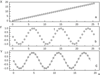
FIG. 3: In these figures are shown the results of numerical integra-tions of the equaintegra-tions of the motion for tracking along a sinusoidal path. In (a) and (b) are shown the tajectoriesxi=x(ti),yi=y(ti). In (c) the trackingyi=y(ti)is compared with the pathy(x) =−sin(x).
therefore, we are able to compute
Fcφ=mρφ˙
˙
φ−a
bψ˙
. (107)
As a fourth example, we consider a sinusoidal pathy(x) =
−Rsin(x/R)withR=1. The equations of motion are, ˙
x = vTsin(Ψ(x))cos(φ(x)), (108) ˙
y = vTsin(Ψ(x))sin(φ(x)). (109) The angles are given by,
tan(φ) = y′(x) =−cos(x), (110)
tan(Ψ) = ρ b =
1+cos2(x)32
bsin(x) , (111)
then
˙
x= vT 1+cos 2(x)
h
b2sin2(x) + (1+cos2(x))3i
1 2
, (112)
˙
y=− vTcos(x) 1+cos
2(x)
h
b2sin2(x) + (
1+cos2(x))3i
1 2
, (113)
which can be integrated to givex(t)andy(t) =−sin(x(t)). The result of numerical integration of the above equation, whichb=1 andvT=1, is shown in figure (3).
Finally, we observe that, from the equation (21), we ob-tain,
maφ¨=−˙λ−ms˙ 2
ρ, (114)
on the system. In the straigh line and the circular trajectories we have ¨φ=0, the angular momentum,pφ=mb2φ˙, is
con-stant under the action of the control system and the constraint reaction and the centrifugal force are in equilibrium.
7. CONCLUSION
The equations of motion for nonholonomic nonau-tonomous controlled systems can be obtained by different methods. Differential geometry approaches to mechanics are usually employed to obtain the equation of motion for this kind of systems [8]. However, we used the vakonomic for-mulation [6], an extension of the lagrangian forfor-mulation in which the lagrangian function is added with a linear com-bination of the constraint conditions. The coefficients of this linear combination are the Lagrange multipliers which are the free parameters that permit to control the system. The next step is to solve the equations of motion using the free parameters to compel the system to follow a prescribed pathway. This procedure, usually called planning or track-ing, requires a prescription that relates the free parameters, or control parameters, of the theory with the input function that describes the chosen trajectory. In this paper, we give a prescription to obtain the control angleΨof the Chaplygin sleigh. This control angle is given by tanΨ= ρb wherebis the radius of gyration of the system andρis the radius of cur-vature of the prescribed pathway. In the appendices we show some examples of Chaplygin systems that can be controlled with the same prescription. All these examples pertain to the class of the unicycles [9]. Some of these examples, the sleigh and the vertical disk, need to be controlled by external force and torque. However, the two wheeled carriage which has an internal degree of freedom can be controlled using internal torque and force. In a next paper, we intend to extend the present formulation to include the process of linear feedback or adaptative control [9]
APPENDIX A: A DISK ROLLING VERTICALLY ON A PLANE WITHOUT SLIPPING [8]
The parameters of this system are the massmof the disc, the momentum of inertiaI1relative to the axis and the mo-mentum of inertiaI2relative to a diameter.
The coordinates of this system are: the cartesian compo-nents(x,y)of the contact point with the plane, the angle of directionφthat the plane of the disk forms with the axisxon the plane and the angleθthat denotes a rotation of the disk. In terms of these coordinates the kinetic energy of the disk reads,
T =1 2
m x˙2+y˙2+I1θ˙2+I2φ˙2
. (A1)
Let~v=s˙sˆbe the velocity of the point of contact or the center of mass of the disk. Its cartesian components are:
˙
x = s˙cosφ, (A2)
˙
y = s˙sinφ. (A3)
Then the motion of the point of contact is constrained by the relation,
−x˙sinφ+y˙cosφ=0. (A4) Besides this anti-transverse motion constraint, the motion of the disk is constrained by the nonslipping condition
˙
s=Rθ˙. (A5)
This last relation can be used to rewrite the kinetic energy in the form
T=1 2
m+ I
R2
˙ s2+I2φ˙2
. (A6)
Defining the new variables,
u1 = r
m+I1
R2s˙, (A7)
u2 =
√
I2φ˙. (A8)
The kinetic energy reads,
T =1 2 u
2 1+u22
. (A9)
The vakonomic formulation can be used to obtain the equa-tions of the motion from the extended lagrangian,
L′=1 2
m+ I1
R2
˙
x2+y˙2+I2φ˙2
+
λ(−x˙sinφ+y˙cosφ). (A10) Similarly as was done for the Chaplygin sleigh, it can be shown thatu1andu2are given by,
u1 =
√
2TsinΨ, (A11)
u2 = √2TcosΨ, (A12)
whereΨis the angle of control given by,
tan(Ψ) = s˙
bφ˙, (A13)
with
b=R s
I2 (I1+mR2)
. (A14)
APPENDIX B: A TWO-WHEELED CARRIAGE ROLLING ON A PLANE WITHOUT SLIPPING [8]
The parameters of this system are the radius R of the wheels, the lenght of the axis 2a, the massmand the mo-ments of inertiaI1andI2of each wheel, the massM, the prin-cipal moments of inertiaIof the axis and platform relative to the vertical axis. In this car the center of mass coincides with the center of the axis between the wheels. Let~v=s˙sˆbe the velocity of the CM of the car. It cartesian components are,
˙
x = s˙cosφ, ˙
which give the anti-transverse constraint
−x˙sinφ+y˙cosφ=0. (B1) The rolling without slipping constraints on the wheels are,
˙
s+aφ˙ = Rθ˙1, (B2) ˙
s−aφ˙ = Rθ˙2. (B3) Defining the new coordinates
θ = 1
2(θ1+θ2), (B4)
ξ = 1
2(θ1−θ2). (B5)
The nonslipping constraints become,
˙
s = Rθ˙, (B6)
aφ˙ = Rξ˙. (B7)
The kinetic energy of the system is
T =1 2 h
m s˙+aφ˙2+m s˙−aφ˙2+Ms˙2+ I1 θ˙21+θ˙22
+ (I+2I2)φ˙2.
(B8)
Changing the variables
˙
θ21+θ˙22=2
˙
θ2+ξ˙2, (B9)
and using the nonslipping constraints we obtain
T =1 2
M+2
m+ I1
R2
˙ s2+
I+2I2+2a2
m+ I1 R2
˙
φ2
. (B10)
Defining the variables
u1 = s
M+2
m+ I1 R2
˙
s, (B11)
u2 = s
I+2I2+2a2
m+ I1 R2
˙
φ. (B12)
The kinetics energy reads,
T =1 2 u
2 1+u22
. (B13)
Using the vakonomic formulation with the extended la-grangian,
L′=T+λ(−x˙sinφ+y˙cosφ), (B14) simmilarly as in the case of the Chaplygin sleigh, we can obtain the equations of the motion and show thatu1andu2 have the forms
u1 = √2Tsin(Ψ), (B15) u2 =
√
2Tcos(Ψ). (B16)
The angle of the controlΨis given by,
tanΨ= s˙
bφ˙, (B17)
with
b= v u u u t
I+2I2+2a2
m+I1
R2
M+2m+ I1
R2
. (B18)
From the extended lagrangian we obtain the angular momen-tum of the system,
pφ=∂
L′
∂φ˙ =
I+2I2+2a2
m+ I1 R2
˙
φ, (B19)
which is not conserved because there is a torque:
ℑ=∂L′
∂φ =−λs˙=p˙φ. (B20)
Using the constraint equationaφ˙=Rξ˙we obtain,
ℑ=−λs˙=
I+2I2+2a2
m+ I1 R2
R a
¨
ξ. (B21)
This result shows that the two-wheeled car can be controlled by an internal torque that produces a difference in the aceler-ations of the wheels ¨ξ=1
2 θ¨1−θ¨2
, and a forceFs.
APPENDIX C: COMPARING THE VAKONOMIC FORMULATION WITH HEURISTIC SOLUTION
In this appendix we show that, for the class of systems considered in this work, the results obtained using the vako-nomic approach can also be obtained with an independent method. The prototype of these systems is the chaplygin sleigh moving on a horizontal plane. Using the same coordi-nates and the notations defined in the section II, the kinetic energy reads
T=1 2
m x˙2+y˙2+ I+ma2φ˙2. (C1) The constraint condition is
−x˙sinφ+y˙cosφ=0 (C2) and the scalar velocity of the point of contact of the knife is
˙
s=x˙cosφ+y˙sinφ. (C3) Using these relations, the knife energy becomes
T =1 2m s˙
2+b2φ˙2
(C4)
whereb2=a2+I/m. The velocity of the center of gyration is
~
thenvT = p
2T/m. We define tanψ= s˙
bφ˙. (C6)
Then(π/2−ψ)is the angle between the velocitiesv~T and
~
vA=s˙sˆ. From the kinetic energy and the definition ofψwe obtain,
˙
s = vTsinψ, (C7)
˙
φ = vT
b cosψ. (C8)
The equations of motion of the system can be obtained using ˙
x=s˙cosφand ˙y=s˙sinφ, that give ˙
x = vTsinψcosφ, (C9) ˙
y = vTsinψsinφ, (C10)
˙
φ = vT
b cosψ. (C11)
These equations of motion depend on two parameters, vT andψwhich must be determined for a prescribed controlled motion of the system along a given path. Let the path be given byy=y(x). Its radius of curvature is
ρ(x) =
1+y′(x)232
y′′(x) . (C12)
which is related to the scalar and angular velocities of the system by
ρ= s˙˙
φ. (C13)
The angleψis then determined by
tanψ=ρ
b. (C14)
The second parameter of control vT can be determined choosing a particular motion along this path. If the ki-netic energy must be constant along the motion, thenvT = p
2T/mis constant. If the scalar velocity ˙smust be constant ˙
s=vs,vT is given by
vT = vs
sinψ (C15)
and the angular velocity is
˙
φ=vs
b cotψ. (C16)
The other equations of motion in this particular case are
˙
x = vscosφ, (C17)
˙
y = vssinφ. (C18)
APPENDIX D: COMPARING THE VAKONOMIC FORMULATION WITH THE LAGRANGE-D’ALEMBERT
PRINCIPLE
The equations of motion for the chaplygin sleigh derived using the vakonomic formulation, equation (21-54), can be
rewritten as
¨
x = −sinφ(x˙cosφ+y˙sinφ)φ˙+ (D1)
aφ˙+λ m
cos(φ)φ˙, (D2)
¨
y = cosφ(x˙cosφ+y˙sinφ)φ˙+ (D3)
aφ˙+λ m
sin(φ)φ˙, (D4)
¨
φ = −1
b2
aφ˙+λ m
(x˙cosφ+y˙sinφ), (D5)
and
˙
λ=
−m
1−a
2
b2
˙
φ+λa b2
(x˙cosφ+y˙sinφ). (D6)
These are control equation that can be used to impose a pre-scribed path to the system.
For autonomous motion we must apply the Lagrange-D’Alembert (LD) principle. For the Chaplygin sleigh the lagrangian is
L = 1 2
m x˙2+y˙2+ ma2+Iφ˙2+ (D7) maφ˙(−x˙sinφ+y˙cosφ), (D8) and the constraint condition reads
Γ x,y,φ,x˙,y˙,φ˙=−x˙sinφ+y˙cosφ=0. (D9) The equations of motion given by the LD principle are
∂L
∂q− d dt
∂L
∂q˙=µ
∂Γ
∂q˙, (D10)
withq=x,y,φ, where µ is a Lagrange multiplier, and the constraint equation:
−x˙sinφ+y˙cosφ=0. (D11) After some algebra, we obtain the equations of motion:
¨
x = −sinφ(x˙cosφ+y˙sinφ)φ˙+aφ˙2cosφ, (D12) ¨
y = cosφ(x˙cosφ+y˙sinφ)φ˙+aφ˙2sinφ, (D13) ¨
φ = −abφ˙2(x˙cosφ+y˙sinφ), (D14) and the force of constraint:
µ=−m
1−a
2
b2
˙
φ(x˙cosφ+y˙sinφ). (D15)
[1] H. Hertz,Die Prinzipien der Mechanik. Gesammelte Werke, vol. 3, Barth, Leipzig, 1894.
[2] H. Goldstein,Classical Mechanics. Addison Wesley Publish-ing Company University Moscow, 1970.
[3] F. Gantmacher,Lectures in Analytical Mechanics. Mir Pub-lisher University Moscow, 1970.
[4] C. Lanczos,The Variational Principles of Mechanics. London: University of Toronto press, 1974.
[5] J. I. Neimark and N. A. Fufaev,Dynamics of Nonholonomic Systems(Translations of Mathematical Monographs, vol. 33), American Mathematical Society, Providence, RI, 1972. [6] V. I. Arnold, V. V. Kozlov and A. I. Neishtadt,Dynamical
Sys-tems Vol. III, Springer-Verlag, New York-Heidelberg-Berlin, 1988.
[7] S. A. Chaplygin, “On theory of motion of nonholonomic sys-tems, The reducing multiplier theorem”. Math. Collection. vol. 28, no. 2, pp. 303-314, 1911.
[8] A. M. Vershik and V. Y. Gershkovich,“Nonholonomic prob-lems and the theory of distributions,” Acta Applic. Math., vol. 12, pp. 181-209, 1988.
[9] C. C. de Wit, B. Siciliano and G. Bastin (The Zodiac),Theory of Robot Control, London: Springer-Verlag, 1997.
[10] P. Pitanga,Quantization of a nonholonomic system with sym-metry. N. Cimento, vol. 109B, pp. 583-594, 1994.
[11] P. Pitanga and P. R. Rodrigues,Projection methods for some constrained systems. Rendiconti di Matematica, vol. 23, pp. 303-328, 2003.
[12] A. S. Sumbatov,Nonholonomic systems. Regular and chaotic dynamics, vol. 7, no. 2, pp. 221-238, 2002.
[13] N. H. Getz and J. E. Marsden, Control for an autonomous bicycle. in Proc. IEEE Int. Conf. Robotics and Automation, (Nagoya, Japan), 1397-1402.
[14] S. Mart´ınez, J. Cort´es and M. de Le´on,The geometric theory of constraints applied to the dynamics of vakonomic mechanical systems. The vakonomic bracket. J. Math. Phys., vol. 41, pp. 2090-2120, 2000.
[15] J. C. Monforte,Geometric, control and numerical aspects of nonholonomic systems, Springer-Verlag, 2002.