❊♥s❛✐♦s ❊❝♦♥ô♠✐❝♦s
❊s❝♦❧❛ ❞❡
Pós✲●r❛❞✉❛çã♦
❡♠ ❊❝♦♥♦♠✐❛
❞❛ ❋✉♥❞❛çã♦
●❡t✉❧✐♦ ❱❛r❣❛s
◆◦ ✹✶✻ ■❙❙◆ ✵✶✵✹✲✽✾✶✵
❙t♦❝❤❛st✐❝ ●r♦✇t❤ ❛♥❞ ▼♦♥❡t❛r② P♦❧✐❝②✿ t❤❡
✐♠♣❛❝ts ♦♥ t❤❡ t❡r♠ str✉❝t✉r❡ ♦❢ ✐♥t❡r❡st
r❛t❡s
❘❡♥❛t♦ ●❛❧✈ã♦ ❋❧ôr❡s ❏✉♥✐♦r✱ ❘✐❝❛r❞♦ ❉✐❛s ❖❧✐✈❡✐r❛ ❇r✐t♦
❖s ❛rt✐❣♦s ♣✉❜❧✐❝❛❞♦s sã♦ ❞❡ ✐♥t❡✐r❛ r❡s♣♦♥s❛❜✐❧✐❞❛❞❡ ❞❡ s❡✉s ❛✉t♦r❡s✳ ❆s
♦♣✐♥✐õ❡s ♥❡❧❡s ❡♠✐t✐❞❛s ♥ã♦ ❡①♣r✐♠❡♠✱ ♥❡❝❡ss❛r✐❛♠❡♥t❡✱ ♦ ♣♦♥t♦ ❞❡ ✈✐st❛ ❞❛
❋✉♥❞❛çã♦ ●❡t✉❧✐♦ ❱❛r❣❛s✳
❊❙❈❖▲❆ ❉❊ PÓ❙✲●❘❆❉❯❆➬➹❖ ❊▼ ❊❈❖◆❖▼■❆ ❉✐r❡t♦r ●❡r❛❧✿ ❘❡♥❛t♦ ❋r❛❣❡❧❧✐ ❈❛r❞♦s♦
❉✐r❡t♦r ❞❡ ❊♥s✐♥♦✿ ▲✉✐s ❍❡♥r✐q✉❡ ❇❡rt♦❧✐♥♦ ❇r❛✐❞♦ ❉✐r❡t♦r ❞❡ P❡sq✉✐s❛✿ ❏♦ã♦ ❱✐❝t♦r ■ss❧❡r
❉✐r❡t♦r ❞❡ P✉❜❧✐❝❛çõ❡s ❈✐❡♥tí✜❝❛s✿ ❘✐❝❛r❞♦ ❞❡ ❖❧✐✈❡✐r❛ ❈❛✈❛❧❝❛♥t✐
●❛❧✈ã♦ ❋❧ôr❡s ❏✉♥✐♦r✱ ❘❡♥❛t♦
❙t♦❝❤❛st✐❝ ●r♦✇t❤ ❛♥❞ ▼♦♥❡t❛r② P♦❧✐❝②✿ t❤❡ ✐♠♣❛❝ts ♦♥ t❤❡ t❡r♠ str✉❝t✉r❡ ♦❢ ✐♥t❡r❡st r❛t❡s✴
❘❡♥❛t♦ ●❛❧✈ã♦ ❋❧ôr❡s ❏✉♥✐♦r✱ ❘✐❝❛r❞♦ ❉✐❛s ❖❧✐✈❡✐r❛ ❇r✐t♦ ✕ ❘✐♦ ❞❡ ❏❛♥❡✐r♦ ✿ ❋●❱✱❊P●❊✱ ✷✵✶✵
✭❊♥s❛✐♦s ❊❝♦♥ô♠✐❝♦s❀ ✹✶✻✮ ■♥❝❧✉✐ ❜✐❜❧✐♦❣r❛❢✐❛✳
Stochastic Growth and Monetary Policy: the
impacts on the term structure of interest
rates
Ricardo D. Brito
†IBMEC and EPGE/FGV
Renato G. Flôres Jr.
EPGE/FGV
April 18, 2001
A bst r act
This paper builds a simple, empirically-veriÞable rational expecta-tions model for term structure of nominal interest rates analysis. It
∗We thank Wolfgang Bühler (University of Mannhein), Rubens Cysne (IBRE), Ruy
Ribeiro (The University of Chicago) and Arilton Teixeira (IBMEC) for helpful comments and suggestions, as well as the participants at the EPGE economics seminar. Ricardo Brito thanks theÞnancial support of CAPES under grant n. BEX0480/98-3 and of BBM.
†Corresponding author: Av. Rio Branco 108/12, 20040-001, Rio de Janeiro, RJ, Brazil.
solves an stochastic growth model with investment costs and sticky
inßation, susceptible to the intervention of the monetary authority following a policy rule. The model predicts several patterns of the
term structure which are in accordance to observed empirical facts:
(i) pro-cyclical pattern of the level of nominal interest rates; (ii)
coun-tercyclical pattern of the term spread; (iii) pro-cyclical pattern of the
curvature of the yield curve; (iv) lower predictability of the slope of the
middle of the term structure; and (v) negative correlation of changes
in real rates and expected inßation at short horizons.
JEL classification: E32; E43; E52
K eywords: Controlled Short Rate; Discontinuous Changes;
Nomi-nal Yield Curve Cyclical Patterns; Expectation Hypothesis Failure
1
I nt r oduct ion
This paper provides an answer to two apparently unrelated questions:
• How can an intertemporal equilibrium model adequatelyÞt an arbitrary
exogenous term structure of interest rates?
• What is the role of monetary policy in determining the term structure
On theÞrst issue, intertemporal general equilibrium modelling of interest
rates still leaves many questions unanswered. As an example, scalar
time-homogenous affine equilibrium models1, famous for their terse description of
an equilibrium economy, which provides tractable and rich analytic results,
because of their constant level of reversion, are intrinsically incapable of
Þtting an arbitrary exogenous term structure. Worse, when tested against
more general scalar speciÞcations, they are usually rejected, suggesting either
the existence of nonlinearity or of omitted variables (Chan et al. [8] or
Aït-Sahalia [1]).
On the second issue, despite the belief that changes in the monetary policy
impact on asset returns in general2 and are a major source of changes in the
shape of the yield curve3, micro-Þnancial models have not accomplished to
properly incorporate it yet. The neglect to deal with macro links leaves
unexplained, or even contradicts, certain stylized facts like the pro-cyclical
nominal interest rate levels, the countercyclical term spread (Fama & French
[13]), or the negative short-run correlation between expected inßation and
1The univariate version of Cox, Ingersoll and Ross [10] can be seen as the most
impor-tant member of the class.
2For example, Thorbecke [28] and Patelis [22] document the existence of a monetary risk
premium and show the role of monetary policy in the predictability of the asset returns.
the expected future real interest rate in the U.K. (Barr and Campbell [3]).
As macro links, omitted variables and constant reversion levels seem to
be the weak points of the scalar time-homogeneous equilibrium models, an
attempt is made here to incorporate a macro monetary policy variable into
an intertemporal equilibrium model. The goal is to get a simple,
empirically-veriÞed rational expectations model for the term structure of nominal interest
rates. A model which allows greatßexibility in the changes of the yield curve,
in response to changes in the macroeconomic environment.
We portray the character ofßuctuations in the term structure of nominal
interest rates, inßation and aggregate output with staggered price contracts
and investment costs, subject to technology shocks and expectational errors
by price bargainers. We end up solving a stochastic growth model, subject to
investment costs and sticky inßation similar to Fuhrer [15], but susceptible
to the intervention of an external authority. The intertemporal optimization
implies a complete description of the multi-period expected returns, and the
model allows the derivation of a nominal term structure which incorporates
the effects of monetary policy. Through discontinuous changes of the
short-term nominal interest rate, the Central Bank forces the left-end of the short-term
net supply of nominal riskless bonds and adds the possibility of jumps in all
forward-looking variables. Given that the monetary authority is constrained
to keep inßation close to zero, future changes in the controlled rate can be
forecasted by looking at the dynamics of the expected inßation and may be
incorporated into the shape of the term structure.
The resulting model extends Balduzzi, Bertola & Foresi’s [2], Rudebusch’s
[25], McCallum’s [18] and Piazzessi’s [23] analyses of the monetary policy
im-pacts on the term structure in the sense that, in an intertemporal equilibrium
framework, it allows the joint explanation of more stylized facts. Indeed,
with a relatively simple model it is shown that the monetary policy has real
effects. We eventually explain: (i) the pro-cyclical pattern of the level of
nominal interest rates; (ii) the countercyclical pattern of the term spread4
(as well as the low sensitivity of long yields to monetary policy changes);
(iii) the pro-cyclical pattern of the curvature of the term structure; (iv) the
lower predictability of the slope of the middle of the yield curve; and (v)
the negative correlation of changes in real rates and expected inßation at
short horizons. Though empirical evidence on these facts is abundant in the
literature (see for example, Campbell, Lo & MacKinlay [7], Fama & French
4The term spread is deÞned as the difference between the yield-to-maturities of a long
[13], Rudebusch [25] and Barr and Campbell [3]) no simple model exists
tak-ing simultaneously into account all them. Moreover, implications of the here
developed model can be explored in a bond pricing context.
The paper has the following structure. Section 2 presents the empirical
patterns, while section 3 reviews the term structure pattern implied by the
plain Real Business Cycle model and points out its nominal indeterminacy.
Both act as a motivation to section 4, where the proposed model is explained
in a representative agent framework. Examples and simulations are
per-formed in section 5, and section 6 concludes. The equivalence between the
representative agent and the competitive formulation of the model is fully
shown in Appendix 1; Appendix 2 explains the numerical method used in
the simulations.
2
Som e St ylized Fact s
This section presents empirical evidences on the movements of the term
struc-ture of nominal interest rates, inßation and output, to which the numerical
predictions of the theoretical models will be subsequently compared. The
rate data available at the FED of Saint Louis’ web site (www.stls.frb.org/fred),
which are taken from the H.15 Release by the Board of Governors. The seven
rates chosen were: 3-Month Treasury Bill Rates (TB3m), 6-Month
Trea-sury Bill Rates (TB6m), 1-Year TreaTrea-sury Bill Rates (TB1), 3-Year TreaTrea-sury
Constant Maturity Rate (CM3), 5-Year Treasury Constant Maturity Rate
(CM5), 7-Year Treasury Constant Maturity Rate (CM7), 10-Year Treasury
Constant Maturity Rate (CM10). T-Bills are secondary market rates on
Treasury securities and the CM rates are constant maturity yields.5.
ForBtj, the nominal price attof the pure discountj−periodbond (or the
zero coupon bond that matures in j periods from t), the yield-to-maturity,
ytj, is the per period interest rate accrued during thej periods:
Btj = 1 +y j t
−j
;
what means the yield-to-maturity is the average return on the bond held
until maturity.
BecauseBtj is known at time t, y j
t is the j−periodriskless nominal rate
5The results to be presented below hold for the Fama & Bliss data set as well, that
prevailing at timetfor repayment att+j. Theone−periodriskless nominal rate prevailing at time t for repayment att+ 1 deserves special notation, it:
Bt1= (1 +it)
−1
,
and is denoted the spot interest rate. For j > l, the l −period nominal
holding return of the j−period bond between t andt+l, hjt+l, t, is the per period interest rate accrued during the l periods:
Btj+−ll Bjt
= 1 +hjt+l, t l.
Given the consumer price index att, Pt, and the inßation between t and
t+l, πt+l, t = Pt + l
Pt −1, the l−period real holding return of the j −period
nominal bond, rjt+l, t, can be analogously deÞned as:
1 +rjt+l, t l = B
j−l t+l
Btj
Pt
Pt+l
= 1 +h
j t+l, t
l
1 +πt+l, t
.
Note that both rtj+l, t,πt+l, t andhjt+l, t only become known at t+l.
The published data are bond-equivalent yields (rBEY) or discount rates
(1 +rBEY ∗ 100j )
1
j −1 and yj = (1 −r
D∗ 100j )
−1
j −1, where j is
time-to-maturity in years. All yields below will be expressed in annualized form.
2.1
P r o-cyclical nom inal int er est r at e levels and
coun-t er cyclical coun-t er m spr ead
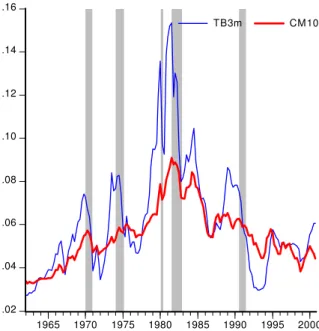
The evolution of the yields-to-maturity of the three-month and of the
ten-year bonds are plotted in Figure 1 with shades added to mark the business
cycles. Every white period points one expansion cycle from trough to peak, as
classiÞed by the NBER. The gray periods mark the contraction periods from
peak to trough. The (i) pro-cyclical pattern of the level of interest rates is
clear: the level increases during expansion and decreases during contraction.
This may be related to the pro-cyclical pattern of the inßation level, as shown
in Figure 2.
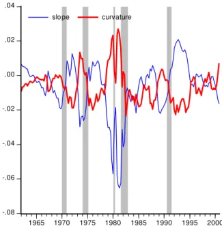
Figure 3 shows the evolution of the slope and the curvature of the yield
curve 6. The (ii) term spread presents a countercyclical pattern: the slope
of the yield curve is big at the trough and decreases during the cycle to
be-come small at the peak. (iii) Curvature seems to decrease along contractions
6The slope of the yield curve is nothing more than the term spread(CM10−T B3m).
(shades) and to increase during expansions.
From (i), (ii) and (iii), it results that the mean term structure at the
trough is a positive sloped, relatively steeper, concave curve, while the mean
term structure at the peak is a negative sloped, relatively ßatter, convex
curve.
2.2
L ower pr edict abilit y of slope of t he m edium t er m
r at es
In the analysis of the term structure, the many versions of the Expectation
Theory of the term structure of interest rates have played an important role.
Loosely stating, the Expectation Hypothesis says that the expected excess
returns on long-term bonds over short term bonds (the term premiums) are
constant over time. This means the term premium can depend on the
ma-turity of the bonds but not on time: Et hjt+l, t−hkt+l, t = f(j, k, l), with
∂f
∂t = 0 ∀ j > k> l
7. In its Pure version (the Pure Expectation Hypothesis,
PEH), it imposes the term premium to be zero.
If any version of the Expectation Hypothesis holds, the slope of the yield
curve is able to forecast interest rate moves, and this predictability is
form along all maturities. For example, to test such a predictability for the
“one-period return”, the PEH reduces to check whether the slope, b, of the
regression:
yl−1
t+ 1−ytl =a+b
yl t−y1t
l−1 +et, (1)
is signiÞcant. Indeed, the above hypothesis implies thatb= 1 for everyl.
Using monthly zero-coupon bond yields over the period 1952:1 to 1991:28,
Campbell, Lo & MacKinlay [7] estimated equations similar to (1) for 2 to
120 months and got the results shown in Table 1.
Besides theb’s being statistically different from 1, the stylized fact that their results bring to scene is the U-shaped pattern of these slope coeffi
-cients: the forecasting power diminishes from the one month to the one year
case and then increases up to the ten years case. This means that (iv) the
predictability of the middle of the yield curve is lower than those of the edges.
2.3
P r incipal com ponent analysis
Are the previous four stylized facts the result of some identiÞable factors? In
this regard, principal component analysis might point at least how many
fac-tors are relevant for empirical term structure motion. Table 2 shows facfac-tors
with a pattern similar to the one uncovered by Litterman & Scheinkman’s
[16].
The Þrst factor has the same sign in all bonds but, different from
Litter-man & ScheinkLitter-man, its impact is higher on the shorter ones. This gives a
different interpretation, that the Þrst factor causes moves in the levels and
in part of the slope changes. The second factor changes sign from the short
end to the long end of the maturities, which means it causes the changes in
slope. Finally, the third factor, which has more impact at the short and long
ends of the term structure, is interpreted as the curvature factor.
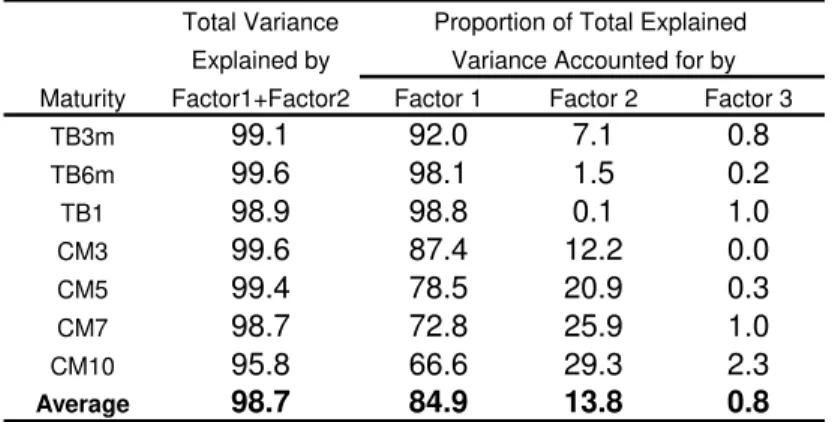
Table 3 shows the proportion of total variance explained by the three
factors.
In the FRED data, the Þrst two factors explain most of the movements
and almost nothing is left to factors 3 and further 9.
Using the FRED 1969-2000 sample and varying frequency, we have
per-formed other principal component analyses (not shown) and obtained that,
once frequency is increased, the Þrst factor loses explanatory power to the
9Litterman & Scheinkman [16] used weekly observations, from January 1984 to June
second and third ones. This is a weak evidence that the 2nd. and 3rd. factors
are more important in explaining short run movements 10.
2.4
N egat ive cor r elat ion of changes in r eal r at es and
expect ed infl at ion at shor t hor izons
Well known in the Þxed income theory is the Fisher hypothesis that there
is no correlation between the expected inßation and the real interest rates:
nominal interest rates change to fully compensate for expected inßation
vari-ations.
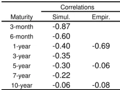
However, this hypothesis is not veriÞed once taken to data: (iv) there
may exist negative correlation between expected inßation and real interest
rate at short horizons. This fact is shown for example by Barr and Campbell
[3], who, working with U.K. data, Þnd correlations of changes in real rates
and expected inßation of -0.69, -0.06 and-0.08 for 1-year, 5-year and 10-year,
respectively. The signiÞcant negative correlation got at a short horizon is
puzzling, since it is expected that investors increase (decrease) their asked
nominal interest rates every time a higher (lower) inßation is expected.
10This is also an evidence that L&S different results might have been caused by the
3
A Sim ple I nt er t em por al Equilibr ium T
he-or y of t he Ter m St r uct ur e wit h pr oduct ion
Because intertemporal optimization models imply a complete description of
the multi-period expected returns, and the term structure of interest rates
is merely the plot of these observed returns, they are suitable as the
micro-foundation of a term structure model.
In the Real Business Cycle (RBC) model with labor supplied inelastically,
the representative agent maximizes:
Et
∞
i=t
βi−tu(c
i) (2)
with: u0(.)≥0, u00(.)<0; subject to the budget constraint:
ct+kt+ 1+b1t+ 1+
∞
j= 2
bt+ 1j (3)
= θtkαt + (1−δ)kt+
1 (1 +πt,t−1)
(1 +it)b0t +
∞
j= 1
Btj
Btj−+ 11
btj −τt;
to the technology shock AR(1) dynamics:
and the transversality conditions:
lim
t→∞β
t
kt= 0; (5)
lim
t→∞β
t
∞
j= 1
Bjt
Pt
bjt = 0; (6)
where:
cstands for real consumption;
k is the real capital stock;
θ is the productivity shock;
0<α<1 is the capital elasticity11; δ is capital depreciation;
(1 +πt,t−1) = PPt
t−1 is the inßation between t−1 and t, with the price
index Pt not known before t;
(1 +it)is the nominal interest rate of theone−periodbond held between
t−1andt, known att−1;
Btj is the nominal price of the j−period bond;
11The production functionf(k,θ) = θtkα
t presents the usual conditions:
bjt is the quantity of the bond the consumer carries from t−1tot, and j
is the number of periods to maturity;
b0
t is the quantity of the bond redeemed att;
andτt are real taxes.
Because labor is inelastically supplied, the production function is
pre-sented in terms of per-capita capital, and the above formulation couches the
case of a constant return-to-scale production function. Also, to make
pre-sentation lighter, instead of the usual normalization of nominal unit price at
maturity, B0
t = 1 ∀ t, we assume that the next-to-mature bond costs one
nominal unit and is worth (1 +it+ 1) nominal units at redemption.
From the above, the representative agent value function can be posed as:
V kt;bjt;j > 0; θt (7)
= max
c, k, b
u(ct) +βEtV(kt+ 1, bjt+ 1> 0,θt+ 1)
−λt
ct+τt+kt+ 1+b1t+ 1+
∞
j= 2b
j
t+ 1−θtkαt −(1−δ)kt
− 1
(1+πt , t−1) (1 +it)b
0
t +
∞
j= 1
Btj Btj + 1−1b
j t
,
u0(c
t) =βEt αθt+ 1kα
−1
t+ 1 + (1−δ) u0(ct+ 1) (8)
u0(c
t)
(1 +it+ 1)
=βEt
1 (1 +πt+ 1,t)
u0(ct+ 1) ; (9) and
u0(ct)
Btj
Pt
=βEt
Bj−1
t+ 1
Pt+ 1
u0(ct+ 1) ∀j; (10) taking prices as given.
Recursion on (10) and the law of iterated expectations implies the l−
period real holding return of thej −periodnominal bond (rjt+l, t):
1 =βlEt
Btj+−ll Btj
Pt
Pt+l
u0(c
t+l)
u0(c
t)
=βlEt 1 +rjt+l, t
lu0(ct+l)
u0(c
t)
∀j and l> 1,
(11)
and gives the whole real term structure implied by the model.
Inasmuch as the yield-to-maturity of everyl−periodbond (yl
t) is known
for certainty at t, 1 +yl t
l
= Bt + l0
Bl
t , it can be taken out of the expectation
1 1 +yl
t l =
Bl t
B0
t+l
=βlEt
1 1 +πt+l, t
u0(c
t+l)
u0(c
t)
∀l; (12)
that provides the whole nominal term structure.
It is trivial that, forl = 1, y1
t =it+ 1; and the above formula simpliÞes to:
1 =βEt 1 +rt1+ 1, t
u0(c
t+ 1)
u0(c
t)
=βEt
1 +it+ 1
1 +πt+ 1, t
u0(c
t+ 1)
u0(c
t)
; (13)
where the spot rate it+ 1can be put outside the expectation if desired. From (12), again by use of the law of iterated expectations, we obtain:
1 1 +y2l
t
2l (14)
= 1
1 +yl t
lEt
1 1 +yl
t+l
l +Covt
βl
1 +πt+l, t
u0(c
t+l)
u0(c
t)
, 1
1 +yl t+l
l ∀l;
which is a generalized version of the PEH, adjusted for the risk premium
Covt β
l
1+πt , t + l
u0(c∗ t + l)
u0(c∗ t) ,
1
(1+yl t + l)
l .
Equation (14) means the PEH holds only in the special cases where the
Also, working on (12), results in the generalized “one-period return” PEH:
1 +yt1 (15)
= 1 +yl t
l
Et
1 1 +yl−1
t+ 1
l−1 +
Covt 1+πt + 1, t1 u0(ct + 1)
u0(ct) ,
1
(1+ylt + 1−1)l−1
Et 1+πt + 1, t1 u
0(ct + 1)
u0(ct)
∀l;
as called by Campbell, Lo and MacKinlay [7]. Again, only when the risk
premium is zero, does the “one-period” PEH hold.
The agent’s optimal conditions allow us to deÞne:
Mlt =βl
u0(c
t+l)
u0(c
t)
(16)
as the stochastic discount function (or the pricing kernel); which in the
present model is equivalent to the intertemporal marginal rate of substitution
in consumption.
3.1
Equilibr ium wit hout ext er nal int er vent ion: infl
a-t ion and nom inal ina-t er esa-t r aa-t e indea-t er m inacy
θt, kt+ 1, ct, it+ 1, πt,t−1, rjt+l,t, b j
t+ 1, τt satisfying the f.o.c.’s and the
market clearing conditions for every t.
Without external intervention, the exogenous supply of bonds is zero:
bjt = 0 ∀ j;
as well as taxes τt = 0, and, given (4), the consumers’ decision simpliÞes
to split wealth between capital and consumption by obeying (8) and the
simpliÞed budget constraint:
ct=θtktα+ (1−δ)kt−kt+ 1, (17)
for everyt.
The initial capital stock, the technology dynamics (4), and the
transver-sality condition (5) deÞne the saddle path expected to be followed by(k , c)
in the system (8) and (17). Substitution of (17) into (8) deÞnes a stochastic
difference equation in k that, given the initial capital stock, initial
technol-ogy and (5), obtains the optimal capital path (k∗
) and provides the inputs to obtain the optimal consumption path(c∗
converges pointwise to a limit distribution when returns are decreasing: k is
pushed to the level kss where the expected marginal productivity of capital
equals the rate of time preference: αkα−1
ss −δ = (1/β)−1 . When
returns-to-scale are constant, they are as well enough to guarantee that the rates of
growth converge pointwise to a limit distribution12.
The application of{c∗
t}
∞
t= 0to (11) endogenously determines the expected
l−period real returns on aj −period nominal bonds fromt tot+l:
1 =βlEt 1 +r j t+l, t
lu0 c∗t+l
u0(c∗
t)
∀j > l; (18)
and gives the whole expected real term structure implied by this equilibrium.
We now deÞne what we understand by neutral values.
D efi nit ion 1 At any time t, the endogenous variables values are neutral,
denoted kN
t+ 1, cNt , iNt+ 1, h
N j
t+ 1,t, πNt+ 1,t, r N j t+ 1,t, b
N j
t+ 1t+ 1 , when the real stock
of bonds is fully rolled over with no portfolio rebalance:
bjt+ 1+ 1−b
j
t = 0 ∀ j.
This means that we qualify all interest rates as neutral when they are
obtained without changes in the bonds’ maturity proÞle. There is no net
ex-ternal intervention, in the sense that the debt-credit proÞle is kept constant.
Thus, within a period, the neutral values are nothing more than those for
which the private sector’s net demand for every maturity bond is zero, what
means people do not sell bonds to Þnance capital or the other way around.
Because there is a stochastic shock in the production function, the
neu-tral real spot rate ßuctuates around a trend deÞned by the optimal capital
path. For example: ifktis increasing along time and the production function
presents decreasing returns-to-scale, the productivity trend is decreasing and
real neutral rate is expected to decrease as the economy tends to the steady
state.
Without an external intervention, the real interest rates, given by (18),
are completely deÞned by (4), (8), (17) and (5). Equation (13) is nothing
more than the Fisher relation that deÞnes next period inßation given the
spot nominal interest rate, or the other way around. Because the expected
spot real interest rate is completely determined by the real factors and is
every time the expected marginal productivity of capital, expected inßation
sensitivity to the level of the nominal interest rate is one, what means no
Although the inßation and nominal rate indeterminacies are a
conse-quence of having more variables than equations, the inclusion of a
cash-in-advance restriction or a Þscalist-theory type of reasoning does not change
the above conclusions. Due to this one-to-one correspondence betweeni and
π, there is no cyclical pattern (i) in the level of the nominal term structure,
(ii) or in that of the term spread, (iii) or in that of the curvature. (iv) The
predictability of the slope of the yield curve is good and equally credible
for every maturity. Moreover, (v) there is no correlation between expected
inßation and the real interest rate since the real interest rates vary with the
marginal productivity of capital and the Fisher hypothesis holds.
Summing up, system (4), (8), (17) and (5) alone does not split the changes
in the nominal rate into changes in the real rate and inßation, and is not of
great use in explaining how monetary policy affects real activity and inßation.
Basically, it assumes neutrality (and superneutrality) and thus thwarts the
possibility that nominal interest rate and inßation vary independently. Quite
unrealistic, inßation reduction to zero can be done in one painless
down-move of the nominal rate to the expected marginal productivity level with
no impact on the real activity.
to couch an ad hoc assumption, and this is done, in conjunction with inßation
stickiness, in section 4.
4
T he M odel
The proposed model describes a closed economy13 with Þrms and capital
accumulation, subject to investment cost and staggered price contracting,
and susceptible to the intervention of a monetary authority. For presentation
purposes, we develop the main ideas in the representative agent framework.
The equivalence with a more detailed economy, where consumers and Þrms
interact in a world of staggered price contracting, is shown in Appendix 1.
13As pointed in Meltzer (1995) pp.50, in an open economy, the exchange rate would be
4.1
T he R eal Side wit h invest m ent cost s
The representative agent maximizes (2), subject to a budget constraint slightly
different from (3):
ct+ kt+ 1+ϕ
kt+ 1
kt
−1
2
+b1t+ 1+
∞
j= 2
bt+ 1j (19)
= θtkαt + (1−δ)kt+
1 (1 +πt,t−1)
(1 +it)b0t +
∞
j= 1
Btj
Btj−+ 11
btj −τt,
and to (4), (5), (6); where: ϕ k+ 1
k −1
2
is the cost of adjustment, and the
other variables have the previous stated meaning.
Now, the representative agent value function can be posed as:
V kt;b j
t; j > 0;θt (20)
= max
c, k, b
u(ct) +βEtV(kt+ 1, bjt+ 1> 0,θt+ 1)
−λt
ct+τt+ kt+ 1+ϕ kt + 1kt −1 2
+b1
t+ 1+
∞
j= 2b
j t+ 1
−θtkαt −(1−δ)kt−(1+π1t , t
−1) (1 +it)b
0
t +
∞
j= 1
Bjt Bj + 1t−1b
j t
;
1 + 2ϕ kt+ 1 kt
−1 1
kt
u0(ct) (21)
= βEt αθt+ 1ktα+ 1−1+ (1−δ)−2ϕ
kt+ 2
kt+ 1
−1 kt+ 2
k2
t+ 1
u0(ct+ 1) ,
replaces (8).
4.2
Cont r act ing Specifi cat ion and t he I nfl at ion D ynam
-ics
Once accounted the investment costs, it is assumed that consumption and
capital goods (c and k) are the same Þnal good, which is the aggregation
of two differentiated goods produced, consumed and invested together in a
Þxed proportion of half each. Although undesirable, the no substitutability
between these (differentiated) component goods simpliÞes matters and
but-tresses a staggered price contracting similar to Fuhrer & Moore [14]. In our
paper, agents negotiate the nominal price contracts of the two Þnal goods,
that remain in effect for two periods. As the model hypothesizes that
pro-duction, consumption and investment are split between these two goods, the
prices:
Pt=X
1 2
t X
1 2
t−1; (22)
where:
Xt is the contract price
andPt is the aggregate price index at t.
Agents set nominal contract prices so that the current real contract price
equals the average real contract price index expected to prevail over the life
of the contract, adjusted for excess demand conditions:
Xt
Pt
=Et
Xt+ 1
Pt+ 1
1 2 X
t−1
Pt−1
1 2
Ytγ; (23)
where the excess demand term Yt was parametrized as Yt = eyt. With this,
yt is the excess demand which can be calculated from the budget constraint
(19) as:
yt = ct+ kt+ 1+ϕ
kt+ 1
kt
−1
2
−(θtktα+ (1−δ)kt) (24)
= − b1
t+ 1+
∞
j= 2
bt+ 1j +τt +
1 (1 +πt,t−1)
(1 +it)b0t +
∞
j= 1
Btj
Btj−+ 11
Considering the expression after the Þrst equality signal, the twoÞrst
mem-bers describe total demand for goods, while the last one (the big expression
between brackets) is the supply of goods. Thus, excess demand can be read
as the private sector’s net demand for bonds, and there is no excess demand
(yt= 0) when variables fromttot+1are neutral (as stated in the DeÞnition).
Equation (23) causes the inßation dynamics:
(1 +πt,t−1) = (1 +πt−1,t−2)
1
2 (1 +E
t[πt+ 1,t])
1 2 (Y
tYt−1)γΩt, (25)
where Ωt is the expectational error, and allows inßation stickiness in the
present model. Note that if expressed in log terms, (25) gives an expression
very similar to the one in Fuhrer & Moore [14], which will be used in the
simulations in section 5 below.
4.3
T he M onet ar y A ut hor it y I nt er vent ion and t he R ole
P layed by M oney
Since we are interested on the study of moves in the yield curve, and not on
the study of optimal monetary policy rules, we don’t care about objective
monetary authority be concerned about inßation, have funds to intervene in
the bond market, and knows its dynamics is given by (25). This being the
case, it is prone to control the one-period spot interest rate toÞght inßation.
Due to operating constraints, it is assumed, without loss of generality, that
it uses the rule:
it+ 1=it+υt, (26)
where:
υt=
0, with probability : (1−ς|πt−1|)
eπt−1
|πt−1|, with probability : ς|πt−1|
;
ande and ς are positive constants 14.
In other words, the spot rate tends to remain constant from period to
period, except for jumps whose probability is an increasing function of the
inßation level. If inßation is positive the eventual jump is positive, and
if inßation there is deßation the jump is negative. When inßation grows,
the probability of jumps increases and so the expected value of the next
14(26) implies the monetary authority inßation targeting is zero. This assumption can
be relaxed by subtracting a constant (or a variable) fromπt
period spot rate. Because inßation is persistent, policy only reverts when
the inßation target has been mostly reached.
The key to our model is monetary authority behavior in the bond market.
It acts buying or selling one-period bonds that pay riskless nominal interest
rate (1 +it+ 1), but risky real interest rate:
1 +it+ 1
1 +πt+ 1,t
,
revealed at t+ 1. Besides, the authority runs no deÞcit, what forces it to charge the individuals a lump sum tax to payoffthe net interest:
τt =
1 +it
1 +πt,t−1
−1 ba
t ∀ t> 0, (27)
where ba
t stands for the per capita bond demand.
As individuals receive the full proceeds of bonds they hold and are charged
lump sum, they choose to long or short the one-period bond once its real
ex-pected return diverges from the exex-pected neutral rate. Thus, although
lend-ing to or borrowlend-ing from the monetary authority are just simple storage in
the aggregate, non-zero net demand for one-period government bonds shows
Not only the above rule makes it easy to forecast tomorrow’s spot rate, but
it also answers for the system stability as long as it guarantees that inßation
does not explode, providing the long run level of the variables. Stability
is the cause for the long rates’ low sensitivity to monetary policy changes:
given the parameters, long run values are implied, and they are the ones that
weight most in the valuation of long term bonds.
No explicit cash motive has been couched; but, without the
cash-in-advance restriction, why would society use money and bear the costs of
monetary policy? Like Woodford [27], it is assumed that modelling the Þne
details of the payments system and the sources of money demand is
inessen-tial to explain how money prices are determined or to analyze the effects of
alternative policies on the inßation path or on other macro variables.
Though buttressing the use of money is not a goal of this paper, we point
out a simple fact of life: money allows specialization, what causes
productiv-ity gains, and that is why society copes with the monetary authorproductiv-ity and its
effects. The economic system is enormously more efficient with than
with-out money and the monetary authority. Loosely modelling, at the real side,
there exist storable goods and two possible production systems. The
more productive than the other, fB, non-monetary, non-specialized system:
fM(k,θ) À fB(k,θ) ∀k. Although storage is also possible, it is greatly
inefficient: production always generates net goods, even after accounting for
all sort of costs and when θ = θinf, while storage just returns the amount stored back.
It is just being assumed here that the gain from being a monetary economy
is discrete and independent of the inßation level, up to an inßation upper
bound above which the economy retraces to the non-monetary system (fB).
The dread to bear such a retrace is what justiÞes the external authority
concern about the inßation level. Due to system stability, it will always be
assumed that inßation is below the upper bound and f =fM.
Since real balance effects do not appear in the inßation dynamics (25),
nor the monetary authority controls the money supply15, the inßation level
determination does not depend upon money demand. The key to analyze
the determination of the inßation level without explicit reference to money
is to model inßation as a function of the level of the real interest rate, and
nominal interest rate as a function of past inßation. This makes real
quanti-ties dependent upon the level of inßation and allows the introduction of the
monetary authority and its policy effects.
4.4
Equilibr ium wit h I nt er vent ion Possibilit y
Equation (19) can be simpliÞed a bit. Because the Central Bank only
inter-venes in theone−periodbond market, onlyb0
t andb1t+ 1can be different from zero and the exogenous supply of the bonds longer than one period is zero:
bjt = 0 ∀j >1. In the representative agent world, equilibrium means:
ba t =b
0
t;
by the intervention policy (27), the economy budget constraint (19) becomes:
ct=θtktα+ (1−δ)kt+b0t − kt+ 1+ϕ
kt+ 1
kt
−1
2
−b1t+ 1 (28) and the excess demand (24):
yt = ct+ kt+ 1+ϕ
kt+ 1
kt
−1
2
−(θtktα+ (1−δ)kt) (29)
with ct, kt+ 1, b1t+ 1 optimally given by (21) and (9). Inßation dynamics simpliÞes to:
(1 +πt,t−1) = (1 +πt−1,t−2)
1
2 (1 +E
t[πt+ 1,t])
1
2 exp γ −b1
t+ 1+b0t−1 Ωt,
(30)
The economy equilibrium sequence θt, it+ 1, ct, kt+ 1, b1t+ 1, πt,t−1, r
j t,t−1 is now given by the system of six simultaneous equations (28), (4), (30), (26),
(21) and (13), and the transversality conditions (5) and (6), given the initial
values for π0,−1, b01, k1 andi1.
4.5
U nder st anding t he m odel dynam ics
The monetary transmission mechanisms are Tobin’s Q theory of investment
and the wealth effects on consumption: the spot rate change sponsors
con-sumption and portfolio responses with real effects.
Although in the representative agent framework, we are able to argue in
terms of the Q-theory of investment. It is possible to get the evolution of
marginal Tobin’s Q:
Q= 1 + 2ϕ k
∗
t+ 1
k∗
t
−1 1
k∗
t
for the optimal capital sequence {k∗
t}
∞
t= 0.
To illustrate the implications of the model, we can make use of phase
diagrams to look at the implied dynamics and the evolution of the term
structure along time. Figure 4 shows the saddle path for the pair (Q, k). Q
is above unit for increasing k and is below unit for decreasing k.
The steady state is the point where the effective output equals the
po-tential one, and there is no excess demand (yt = 0). In this case, at every
technology shock that improves (worsens) efficiency, ∆Q = 0 moves north-east (southwest). The effect is similar in the case of monetary interventions
that lower (rise) the real interest rate. However, as these last interest changes
are transitory, a backwards move in the ∆Q = 0 curve is expected to take place sometime in the future.
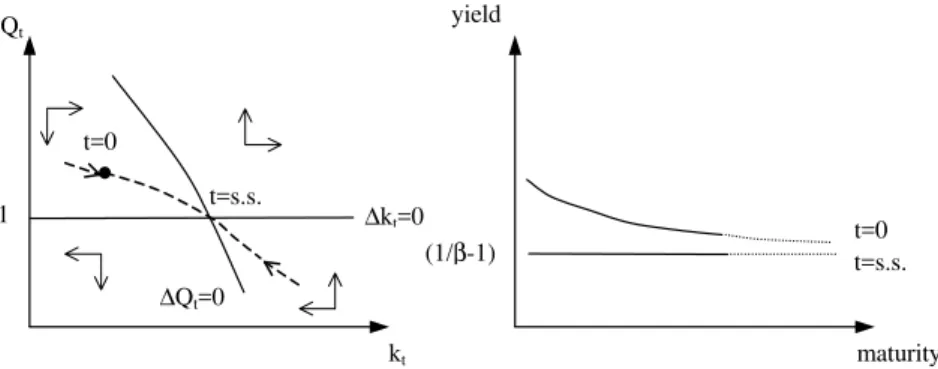
The variety of term structure shapes and dynamics allowed makes
com-prehensive illustration unfeasible, but intuition can be gained in the analysis
of simple cases. For example, without inßation, the left diagram in Figure 5
shows the dynamics of Q and K, and the right diagram shows the implied
dynamics of the real term structure. It is the case without intervention of an
economy’s growth path.
ßatter as the economy comes close to the steady-state (t = s.s.), since the ratios of two different time consumptions approach unity (and the real yields
approach β−1
for every maturity). ytj is given by:
yjt =
1
β Et
u0(c
t+j)
u0(c
t)
−1 j
−1, ∀j,
and at t = 0 (k0 below kss), the real term structure is downward sloping
sincectis expected to grow at decreasing rates. The just described expansion
path contrasts the initial negative slope of the real term structure with the
empirical initial positive slope of the nominal term structure shown in section
2. This stress our that plain RBC models, or the univariate version of Cox,
Ingersoll and Ross, aren’t good enough to explain the nominal term structure.
Something practitioners in the Þnancial markets are well aware of.
Figure 6 shows what happens when a temporary increase in the real spot
interest rate is expected at a certain date and for a certain period, due to
a tight of the Central Bank to Þght increasing inßation16: once the tight
becomes expected, Q jumps down and K begins to decrease up to the time
when the change happens (at T). Between the effective tight and the time
16This is an unrealistic exercise with didactical purposes only. Central Bank’s
policy is again loosened,Qincreases, whileK Þrst decreases, to increase after
Q reaches unit. (Q, K) changes happen so that when policy reverts to loose
again (at T’), the pair is over the original saddle and goes to the steady-state.
Figure 7, on the other hand, shows what happens when the time of the
target is uncertain. Once the change becomes justiÞable by “high” inß
a-tion, Q jumps to an intermediary saddle path, located in accordance with
the probability of change. While the change does not happen, inßation is
increasing and the intermediary saddle moves southwest (due to the
increas-ing probability), brincreas-ingincreas-ing together the pair (Q, K). Once the tight takes
place (at T), Q jumps again to a point that depends on the expected future
monetary policy.
The combination of the real spot interest rate with the inßation dynamics
allows to obtain all sort of shapes for the term structure.
4.6
Explanat ion of t he st ylized fact s
The Þve stylized facts can be explained by our model.
With the spot-rate exogenously Þxed, sticky inßation and adjustment
costs, the Fisher hypothesis of constant real interest rates can’t hold and the
of capital for a while. A positive (negative) inßation shock not
accompa-nied by a spot-rate jump lowers (raises) the real interest rate below (above)
the present capital productivity level and sponsors capital investment
(disin-vestment). But, due to increasing investment costs, capital does not adjust
instantaneously.
Inasmuch as the expected inßation is pro-cyclical, (i) the nominal interest
rates level is high in the peak and low in the trough of the business cycle.
Pro-cyclical nominal rates means existing bonds are expected to lose
(gain) value during the expansion (contraction) as the rates increase
(de-crease). The negative of the modiÞed duration of the bond, deÞned as:
−M.Duration= ∂B
∂y
1
B =−j
1 (1 +y)
shows that longer bonds are relatively more affected by the expected future
change in the level of the term structure. Thus, (ii) the countercyclical
pattern of the term spread can be explained as a “level upside-move risk”
that is proportional to the bond duration. Due to system stability, people
believe there are upper and lower bounds for the expected inßation and the
inßation itself. When the economy begins an expansion, the nominal interest
rates and inßation levels are low, and inßation is expected to grow. Spot rate
jumps in the near future will have positive signs, this meaning lower bond
prices and capital losses for the long maturities bond holders, who charge
their borrower for that. As expansion takes place, inßation increases, followed
by the spot-rate. Since there is a perceived upper limit for the inßation, the
‘level upside-move risk’ decreases along this path, and the reduction in the
term spread is consistent. The description of the recession goes along the
same lines.
Convexity, deÞned as:
Convexity = ∂
2B
∂y2
1
B =j(j+ 1)
1 (1 +y)2,
shows that the (iii) pro-cyclical curvature is explained by the same ‘level
upside-move risk’.
The way nominal spot interest rate is modiÞed gives rise to a (iv) negative
short-run correlation between expected inßation and expected future real
interest rate, since inßation innovations are not instantaneously transmitted
The monetary authority operating procedure, together with inßation
stick-iness and the system stability seem enough to justify (v) the better
pre-dictability of the slope of the yield curve at the short- and at the long-ends
respectively (or the worse predictability of the slope of the middle of the yield
curve). The monetary authority operating procedure and inßation stickiness
imply the persistency of monetary policy and that inßation lasts for a while,
explaining the good predictability of the slope at the short-end of the term
structure. At the long-end, because the system is stable, long-term bond
yields are mainly deÞned by the long run values, and shocks have a
transi-tory and small impact. Investors have reasonable certainty about inßation
and the spot rate in the near future, as well as in the long run given the
system is stable. However, due to the same inßation stickiness and
operat-ing procedures, people is uncertain about how long it takes for a policy to
reach its goal and when it is going to be reverted, these being the causes for
increased middle term uncertainty.
In the context of the present model, we have three shocks that can be
decomposed into orthogonal factors, but not interpreted as a factor itself.
Our structural shocks are not orthogonal: technology shocks may cause
Factor 1 for example, which affects all yields with the same sign but affects
long yields less, might have considerable weight on the technology, ε, and
expectational error shock,ω,since both impact more short rates and die out
with time. We thus let factor interpretation for further research.
5
M odel Solut ion, Simulat ions and Pr
edic-t ions
Equations (4), (13), (25), (26), (21) and (28) form a non-linear stochastic
difference system with rational expectations that can be numerically solved
according to Novales et al.[21] by use of Sims [26] method described in the
Appendix 2.
Numerical exercises reported below used the following set of parameters:
α = 0.4 and δ = 0.025 are standard calibration parameters for quarterly frequency data. Values for σ = 2 and β = 0.995 are in accordance with Fuhrer’s [15] similar model. A ϕ= 380 seems reasonable in view of the ex-isting literature (see Dixit & Pindyck [11]). Finally, ρ = 0.9 andγ = 0.024
were estimated from data. The procedure performed to estimate ρ was close
quarter, we have logθt−logθt−1 = (logYt−logYt−1), an expression which allows building up theθt series, whereY is the gap between GNP and
poten-tial GNP; then, with the obtained θ0s, ρ is estimated. The γ was estimated
by instrumental variables using CPI inßation seasonally adjusted and the
negative of the System Open Market Accounting Holdings (per-capita and
discounted a trend).
5.1
Exper im ent s
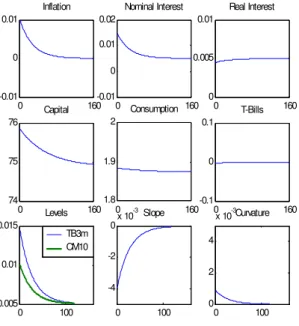
Figures 8 and 9 illustrate the dynamics of two experiments: (i) a disinßation
experiment, when inßation and capital start above the steady state (Figure
8), and (ii) an expansion experiment, when capital as well as inßation start
below the steady state level (Figure 9).
As shown in Figure 8, the level of the nominal interest rates are initially
high, but the short real interest rate is expected to increase and inßation to
decrease. The evolution of the term structure is illustrated in the Þgure.
In Figure 9, capital and consumption increase along time, while the real
interest rates decreases.
In both cases the impulse response functions seem to describe real data17.
5.2
Simulat ion wit h t he U .S. dat a
It is worth asking if the numerical predictions of the theoretical model present
patterns similar to the stylized facts in section 2.
In a attempt to test whether the model reproduces the data pattern,
we have performed the following Monte Carlo exercise: given date t states
πt−1,t−2, b0t, kt and it+ 1, to build the joint expectation conditional on the available information set, 500 random paths of the model’s variables were
obtained by simulating the system 10 years ahead, using shocks got from a
bivariate normal random vector with covariance matrix 00725
−.002 .00579
,
which is the estimated matrix from the above residual series. With the joint
expectation of the model variables calculated, the nominal term structure on
t was then deÞned by the yields of the many maturity bonds:
ytj =
1
β Et
1 1 +πt+j,t
u0(c
t+j)
u0(c
t)
−1 j
−1, ∀j = 1, ...,40.
To move fromt tot+ 1,and calculate the term structure on t+ 1as just described, we assumed the realized shock to be the residual shock (εt, ωt)
estimated from equations (4) and (25) from 1969:1 to 2000:4. The ε was as
the residual of the equation for estimating ρ. The ω was the residual of the
equation for estimating γ (see Section 5 introduction).
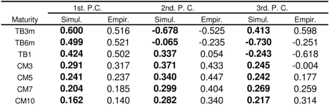
The results are sensible and “close” to the qualitative pattern documented
in Section 2. Tables 4 and 5 below show the relative importance of the factors
and their respective eingenvectors.
The simulation also reproduces the correlation between expected inßation
and real interest rate. Table 6 shows the obtained values, which are close to
the U.K. empirical ones.
6
Conclusion
The simple macro model developed in this paper is able to Þt the empirical
term structure of interest rates in different situations. It doesn’t focus on the
behavior of some instantaneous spot rate process, derived from a particular
equilibrium model, to obtain the term structure, as usual in the literature.
Instead, it sees the spot-rate as an instrument of the monetary authority,
who controls it to match the goal of low price variation. A key behavioral
rule introduces the needed ßexibility in linking macro variables changes to
state variables may be forecasted with a high degree of accuracy, as well as
the future changes in the spot rate. To obtain the term structure, people does
take into account the current drift of the inßation and what future monetary
policy actions it implies.
Simulations produced results qualitatively close to several stylized facts:
(i) pro-cyclical pattern of the level of nominal interest rates; (ii)
counter-cyclical pattern of the term spread (as well as low sensitivity of long yields
to monetary policy changes); (iii) pro-cyclical pattern of the curvature of
the term structure; (iv) lower predictability of the slope of the middle of the
yield curve; and (v) negative correlation of changes in real rates and expected
inßation at short horizons. Other empirical experiments may show how good
is the proposed model toÞt various empirical sets of data. From a theoretical
viewpoint, new and probably more accurate, bond pricing mechanisms can
Appendices
A
The Competitive Problem
The equivalence of the representative consumer with a competitive
econ-omy is shown below. As usual in the competitive framework, consumers and
Þrms maximize their objective function taking prices as given. Without loss
of generality, it is assumed that the Þrms are the owners of capital and are
all equity Þnanced18.
A .1 Consum er s
The consumers budget constraint is given by:
ct+qtzt+ 1+b1t+ 1+
∞
j= 2
bt+ 1j (A.1)
= (qt+dt)zt+wtlt+
1 (1 +πt,t−1)
(1 +it)b0t +
∞
j= 1
Btj
Btj−+ 11
btj −τt;
and the transversality conditions (6) and:
18For the Þrms decision between equity and debt in a framework similar as ours, see
lim
t→∞β
t(q
t+dt)zt= 0; (A.2)
where: q is the real stock price;z is the quantity of the stocks; d is the real
dividends; wt denotes the real wage; andlt is the amount of labor.
This results in the consumers’ optimal allocation rules:
1 =βEt
qt+ 1+dt+ 1
qt
u0(c
t+ 1)
u0(c
t)
; (A.3)
and (9), (11), taking prices as given.
Given that consumers do not enjoy leisure,lt = 1 ∀ t.
A .2 Fir m s
At theÞrm’s side, the law of motion for its capital stock is:
Kt+ 1=Ktd+I d
t = (1−δ)Kt+Itd;
where:
Kt+ 1 is the capital stock to be used next period;
Kd
t stands for used capital demanded for use next period; and
Id
DeÞne the gross proÞts to be given by:
Prof itst =f(Kt, lt,θt)−wtlt.
AssumingÞrms are all equity Þnanced, the following identity holds:
Prof itst=RE+dtzt,
and the ex-dividend relation is:
qtzt+ 1=pk, tKt+ 1;
with RE for retained earnings and pk, t being the real price for used capital.
Financing of new and used capital obeys:
pk, tKtd+I d t +ϕ
Kt+ 1
Kt
−1
2
=RE+qt(zt+ 1−zt) + (1−δ)pk, tKt;
Nt = f(Kt, lt,θt) + (1−δ)pk, tKt−wtlt−pk, tKtd
− (Kt+ 1−(1−δ)Kt) +ϕ
Kt+ 1
Kt
−1
2
= dtzt+qt(zt−zt+ 1)
Thus, theÞrm problem can be posed as:
W(Kt) = max
k, l {Nt+Et[M1tW(Kt+ 1)]},
with M1t treated parametrically by Þrms19, and gives the Þrst order
condi-tions:
wt=f(Kt, lt,θt)−f1(Kt, lt,θt)Kt;
pk, t =Et[M1tW1(kt+ 1)] ; (A.4)
1 + 2ϕ Kt+ 1 Kt
−1 1
Kt
The envelope is:
W1(kt) =f1(Kt, lt,θt)−2ϕ
Kt+ 1
Kt
−1 Kt+ 1
K2
t
+ (1−δ)pk, t. (A.6)
Substituting the envelope forwarded one period into (A.4) as well as (A.4)
into (A.5) results the Þrms’ optimal decision rules:
pk, t (A.7)
= Et M1t f1(Kt+ 1, lt+ 1,θt+ 1)−2ϕ
Kt+ 2
Kt+ 1
−1 Kt+ 2
K2
t+ 1
+ (1−δ)pk, t+ 1
and
1 + 2ϕ Kt+ 1 Kt
−1 1
Kt
=pk, t;
taking prices as given.
qt+ 1+dt+ 1
qt
M1t
=
f1(Kt+ 1, lt+ 1,θt+ 1)−2ϕ KKt + 2t + 1 −1 KKt + 22 t + 1 + (1
−δ)pk,t+ 1
pk,t
M1t ;
andpk, t is equal to Tobin‘s marginal Q is given by:
pk, t = 1 + 2ϕ
Kt+ 1
Kt
−1 1
Kt
=Q;
A .3 Com p et it ive Economy Equilibr ium
An equilibrium is deÞned as a set of stochastic processes
rjt,t+l, qt, pk,t, zt, b j
t+ 1, k+ 1, ct, lt satisfying the f.o.c.’s and the market
clearing conditions.
Becauselt= 1 ∀t, we can argue in terms of per capita capital kt.
To make things simpler, assume there is no issue of new shares and the
ÞrmÞnances itself by retained earnings:
zt+ 1=zt= 1,
qt=pk,tkt+ 1 ∀t. The economy resources constraint is thus:
f(kt,θt) =ct+ (kt+ 1−(1−δ)kt) +ϕ
kt+ 1
kt
−1
2
, (A.8)
and given the model parameters, the economy equilibrium conditions become:
pk,t =βEt f1(kt+ 1,1,θt+ 1)−2ϕ
kt+ 2
kt+ 1
−1 kt+ 2
k2
t+ 1
+ (1−δ)pk,t+ 1
u0(c
t+ 1)
u0(c
t)
and
1 + 2ϕ Kt+ 1 Kt
−1 1
Kt
=pk, t,
with ct given by (A.8). A system of two simultaneous equations that can be
solved for the two unknowns pk andk (or Qand k).
B
Numerical Solution
(4), (13), (25), (26), (21) and (28) can be linearized around the steady and
solved by some linear solution methods with reasonable precision, as shown
in Novales et al. [21].
We have chosen to use Sim’s [26] method to solve our model. The
proce-dure consists of dealing with each conditional expectation and the associated
expectational error as additional variables, adding to the system an
equa-tion that deÞnes the expectational error. In our case, we have deÞned the
variables:
W1t =Et αθt+ 1ktα+ 1−1+ (1−δ)−2ϕ
kt+ 2
kt+ 1
−1 kt+ 2
k2
t+ 1
u0(ct+ 1) ,
W2t=Et
1 (1 +πt+ 1,t)
u0(ct+ 1) ,
W3t=Et[πt+ 1,t] ;
and the respective expectational errors η1t, η2t, η3t.
The resulting linearized system is then written as::
where:
yt = (ct−css, kt+ 1−kss, bt+ 1−bss, W1t−W1ss, W2t−W2ss, it+ 1−iss,logθ,
πt,t−1, W3t, bt−bss)is the vector of variables determined within the model
(inclusive W, but except η) and Γ0 and Γ1 are the matrices containing the system linearized coefficients.
IfΓ0 is invertible (and it is):
yt =Γ
−1
0 Γ1yt−1+Γ −1
0 Ψzt+Γ
−1
0 Πηt =Γ1yt−1+Ψzt+Πηt
andΓ1 has a Jordan decompositionΓ1=PΛP−1. DeÞning wt=P−1yt, we obtain:
wt=Λwt−1+P −1
Ψzt+Πηt
where, for every eigenvalueλj of Γ1 we have an equation:
wjt =λjjΛwj,t−1+Pj. Ψzt+Πηt
where Pj. denotes the j-th row of P−1.
than β−1
2, forwj,with |λjj|>β−12, we need have:
wjt =Pj.yt = 0, ∀t
which provides the system stability conditions.
Using the notation P = [P•S, P•U] and P−1 = [
PS•
PU•
], where U stands for “unstable”, the system can be written as:
wS,t=ΛSwS,t−1+ I −Φ P−1Ψzt; (B.1)
where: Φ=PS•Πη PU•Πη −1.
To arrive at an equation iny, we use y=P w to transform (B.1) into:
yt=P•SΛSPS•yt−1+ P•SPS•−P•SΦPU• Ψzt,
which can be solved after imposing:
R efer ences
[1] Aït-Sahalia, Y., 1996. Testing Continuous-Time Models of the Spot
In-terest Rate. Review of Financial Studies 9, 385-426.
[2] Balduzzi,P., Bertola, G., Foresi, S., 1993. A Model of Target Changes
and The Term Structure of Interest Rates. NBER Working Paper
No.4347.
[3] Barr, D., Campbell, J., 1997. Inßation, Real Interest Rates, and the
Bond Market: a Study of the UK Nominal and Index-Linked
Govern-ment Bond Prices. Journal of Monetary Economics 39, 361-383.
[4] Black, R., Macklem, T., Rose, D., 1997. On Policy Rules for Price
Sta-bility. In: Bank of Canada (Ed.), Price stability, inßation targets and
monetary policy. Bank of Canada, Ottawa.
[5] Brock, W., 1979. An Integration of Stochastic Growth Theory and
the Theory of Finance, Part I: The Growth Model. In: Green, J.,
Scheinkman, J. (Ed.), General Equilibrium, Growth and Trade.
[6] Brock, W., Turnovsky, S., 1981. The Analysis of Macroeconomic Policies
in Perfect Foresight Equilibrium. International Economic Review 22, 1,
179-209.
[7] Campbell, J., Lo, A., MacKinlay, A., 1997. The Econometrics of
Finan-cial Markets. Princeton University Press, Princeton, NJ.
[8] Chan, K., Karolyi, A., Longstaff, F., Sanders, A., 1992. An Empirical
Comparison of Alternative Models of the Short-Term Interest Rate. The
Journal of Finance 47, 1209-1227.
[9] Cooley, T., Prescott, E., 1995. Economic Growth and Business Cycles”.
In: Cooley, T., Prescott, E. (Ed.), Frontiers of Business Cycle Research.
Princeton University Press, Princeton, NJ.
[10] Cox, J., Ingersoll, J., Ross, S., 1985. A Theory of the Term Structure of
Interest Rates. Econometrica 53, 385-407.
[11] Dixit, A., Pindyck, R., 1994. Investment Under Uncertainty. Princeton
University Press, Princeton, NJ.
[12] Fama, E., Bliss, R., 1987. The Information in the Long-Maturity
[13] Fama, E., French, K., 1989. Business Conditions and Expected Returns
on Stocks and Bonds. Journal of Financial Economics 25, 23-49.
[14] Fuhrer, J., Moore,G., 1995. Inßation Persistence. The Quarterly Journal
of Economics February, 127-159.
[15] Fuhrer, J., 1997. Towards a compact, empirically-veriÞed rational
expec-tations model for monetary policy analysis. Carnegie-Rochester
Confer-ence Series on Public Policy 47, 197-230.
[16] Litterman, R., Scheinkman, J., 1991. Common Factors Affecting Bond
Returns. Journal of Fixed Income 1, 54-61.
[17] Mankiw, N., Miron, J., 1986. The Changing Behavior of the Term
Struc-ture of Interest Rates. The Quarterly Journal of Economics May,
211-228.
[18] McCallum, B., 1994. Monetary Policy and the Term Structure of Interest
Rates. NBER Working Paper No.4938.
[19] McCulloch, J., Know, H., 1993. U.S. Term Structure Data, 1947-1991,”
[20] Meltzer, A., 1995. Monetary, Credit (and Other) Transmission
Processes: A Monetarist Perspective. The Journal of Economic
Per-spectives 9, 2, 49-72.
[21] Novales, A., Dominguez, E., Perez, J., Ruiz, J., 1999. Solving Nonlinear
Rational Expectations Models by Eigenvalue-Eigenvector
Decomposi-tions. In: Marimon, R., Scott, A. (Ed.), Computational Methods for
the Study of Dynamics Economics. Oxford University Press, Oxford.
[22] Patelis, A., 1997. Stock Return Predictability and the Role of Monetary
Policy. The Journal of Finance 52, 1951-1972.
[23] Piazzesi, M., 2000. An Econometric Model of the Yield Curve with
Macroeconomic Jump Effects. Stanford University, Mimeo.
[24] Romer, D., 1996. Advanced Macroeconomics. McGraw-Hill, New York,
NY.
[25] Rudebusch, G., 1995. Federal Reserve Interest Rate Targeting, Rational
Expectations, and the Term Structure. Journal of Monetary Economics
[26] Sims, C., 2000. Solving Linear Rational Expectations Models. Journal
of Economic Dynamics and Control, forthcoming.
[27] Woodford, M., 1997. Doing Without Money: controlling inßation in a
post-monetary world. NBER Working Paper No. 6188.
[28] Thorbecke, W., 1997. On Stock Market Returns and Monetary Policy.
Figures and Tables
.02 .04 .06 .08 .10 .12 .14 .16
1965 1970 1975 1980 1985 1990 1995 2000
TB3m CM10
Figure 1: Evolution of U.S. nominal yields from 1962:01 to 2000:04
-.08 -.04 .00 .04 .08 .12 .16
1965 1970 1975 1980 1985 1990 1995 2000 inflation
-.08 -.06 -.04 -.02 .00 .02 .04
1965 1970 1975 1980 1985 1990 1995 2000 slope curvature
Figure 3: Evolution of U.S. slope and curvature of the term spread from
1962:03 to 2000:04
2 3 6 12 24 48 120
b .502 .467 .320 .272 .363 .442 1.402 (s.e.) (.096) (.148) (.146) (.208) (.223) (.384) (.142)
Maturity 1st. P.C. 2nd. P. C. 3rd. P. C.
TB3m 0.516 -0.525 0.598
TB6m 0.521 -0.235 -0.251
TB1 0.502 0.054 -0.618
CM3 0.317 0.433 -0.004
CM5 0.237 0.447 0.177
CM7 0.185 0.404 0.259
CM10 0.140 0.340 0.314
Table 2: Empirical First three principal components (or eigenvectors whith
largest eigenvalues) - quartely U.S. nominal yields from 1969:03 to 2000:04
Total Variance Proportion of Total Explained Explained by Variance Accounted for by Maturity Factor1+Factor2 Factor 1 Factor 2 Factor 3
TB3m 99.1 92.0 7.1 0.8
TB6m 99.6 98.1 1.5 0.2
TB1 98.9 98.8 0.1 1.0
CM3 99.6 87.4 12.2 0.0
CM5 99.4 78.5 20.9 0.3
CM7 98.7 72.8 25.9 1.0
CM10 95.8 66.6 29.3 2.3
Average 98.7 84.9 13.8 0.8
Table 3: Empirical Relative Importance of the Empirical Factors (%)
-quartely U.S. nominal yields from 1969:03 to 2000:04
kt
Qt
∆kt=0
∆Qt=0
t=0
t=s.s. 1