What measure of inflation should a developing country central bank target?

What measure of inflation should a developing country central

bank target?

Rahul Anand

a

, Eswar S. Prasad

b,n

, Boyang Zhang

c

a_{International Monetary Fund, Washington D.C. 20431, USA}

b_{Dyson School of Applied Economics and Management and Department of Economics, 301A Warren Hall, Cornell University, Ithaca,} NY 14853, USA

c_{Department of Economics, Cornell University, Ithaca, NY 14853, USA}

a r t i c l e

i n f o

Article history:

Received 4 December 2012 Received in revised form 17 June 2015

Accepted 19 June 2015 Available online 2 July 2015

Keywords: Inflation targeting Monetary policy framework Core inflation

Headline inflation Financial frictions

a b s t r a c t

In closed or open economy models with complete markets, targeting core inflation enables monetary policy to maximize welfare by replicating the flexible price equilibrium. We analyze this result in the context of developing economies, where a large proportion of households are credit constrained and the share of food expenditures in total consumption expenditures is high. We develop an open economy model with incomplete financial markets to show that headline inflation targeting improves welfare outcomes. We also compute the optimal price index, which includes a positive weight on food prices but, unlike headline inflation, assigns zero weight to import prices.

&2015 Elsevier B.V. All rights reserved.

1. Introduction

Most central banks view low and stable inflation as a primary, if not dominant, objective of monetary policy. In the existing literature, the choice of price index to target has been guided by the idea that inflation is a monetary phenomenon. Core inflation (excluding food, energy, and other volatile components from headline CPI) has been viewed as the most appropriate measure of inflation since fluctuations in food and energy prices represent supply shocks and are non-monetary in nature (Wynne, 2008). Moreover, since these shocks are transitory, highly volatile, and do not reflect changes in the underlying rate of inflation, they should not be a part of the targeted price index (Mishkin, 2007,2008).

Previous authors have used models with price and/or wage stickiness to show that targeting core inflation maximizes welfare. Existing models have looked at complete market settings where price stickiness is the only distortion (besides monopoly power). Infrequent price adjustments cause mark-ups to fluctuate and also distort relative prices. In order to restore the flexible price equilibrium, central banks should try to minimize these fluctuations by targeting sticky prices (Goodfriend and King, 1997,2001).

Using a New Keynesian model,Aoki (2001) demonstrates that targeting inflation in the sticky price sector leads to macroeconomic stability and welfare maximization. Targeting core inflation is equivalent to stabilizing the aggregate output gap as output and inflation move in the same direction under complete markets.Benigno (2004)argues that in a common currency area the central bank should target an index that gives higher weight to inflation in regions with a higher degree of

Contents lists available atScienceDirect

journal homepage:www.elsevier.com/locate/jme

Journal of Monetary Economics

http://dx.doi.org/10.1016/j.jmoneco.2015.06.006 0304-3932/&2015 Elsevier B.V. All rights reserved.

n

nominal rigidity, effectively ignoring exchange rate and commodity price fluctuations. In a more general multi-sector setting,Mankiw and Reis (2003)show that, in order to improve the stability of economic activity, the targeted“stability”

price index should put more weight on sectors that have sluggish price adjustment, are more procyclical, and have a smaller weight in the consumer price index.

The results from the prior literature generally rely on the assumption that markets are complete (allowing households to fully insure against idiosyncratic risks). The central bank then only needs to tackle the distortions created by price stickiness. However, in developing economies, a substantial fraction of agents are unable to smooth their consumption in a manner consistent with the permanent income hypothesis. Moreover, developing economies have other structural differences from advanced economies, including the relatively high share of food in household consumption expenditures.

In this paper, we provide an analytical framework for determining the optimal price index for developing economy central banks to target. The paper makes three main contributions. First, it generalizes the results of Aoki (2001)and

Benigno (2004) by developing a model that encompasses their frameworks. Second, it shows that incomplete financial markets and other characteristics of developing economies substantially alter the key results. Third, it derives optimal price indexes and compare them with feasible rules such as headline inflation targeting that also improve welfare relative to core inflation targeting but are easier for central banks to communicate and implement.

Our model has three sectors to make it more representative of the structures of developing economies. First, the food (or informal) sector, which comprises a large fraction of the economy and where prices are flexible. Workers in this sector live hand-to-mouth, i.e., they have no access to credit markets and simply consume their current labor income. Second, the sticky price (or formal) sector that is subject to productivity and mark-up shocks, and where workers do have access to credit markets. Third, a sector that is open to foreign trade and where prices are flexible but also highly volatile. This sector, which proxies for the commodity-producing sector, faces large external shocks.

Financial frictions that result in consumers being credit constrained have not received much attention in models of inflation targeting. When markets are not complete and agents differ in their ability to smooth consumption, their welfare depends on the nature of idiosyncratic shocks. Thus, this model also allows us to analyze the welfare distribution under alternative inflation targeting rules. Under incomplete markets, household income, which is influenced by the nature of shocks and the price elasticity of the demand for goods, matters for consumption choices. For instance, a negative productivity shock to a good with a low price elasticity of demand could increase the income of net sellers of that good and raise the expenditure of net buyers of that good.

Our model incorporates other important features relevant to developing economies. In these countries, expenditure on food constitutes 40–50 percent of household expenditures, compared to 10–15 percent in advanced economies. Low price and income elasticities of food expenditures as well as low income levels make the welfare of agents in developing economies more sensitive to fluctuations in food prices. These features imply that agents factor in food price inflation while bargaining over wages, thus affecting broader inflation expectations (Walsh, 2011). Thus, in developing economies even inflation expectation targeting central banks must take into account food price inflation.

Our key result is that in the presence of financial frictions targeting headline CPI inflation improves aggregate welfare relative to targeting core inflation (i.e., inflation in the sticky price sector). Lack of access to financial markets makes the demand of credit-constrained consumers insensitive to interest rates. These consumers' demand depends only on real wages, establishing a link between aggregate demand and real wages. Thus, the relative price of the good produced in the flexible price sector not only affects aggregate supply but, through its effects on real wages, also influences aggregate demand.

Our model allows us to compute optimal price indexes that maximize welfare. The optimal price index also includes a positive weight on food prices but, unlike headline inflation, generally assigns zero weight to import prices. This is because agents in that sector have access to financial markets and, unlike in the case of food, the price elasticity of the demand for goods produced in this sector is high.

These results differ from those of the prior literature based on complete markets settings. For instance, inAoki's (2001)

model, relative prices of the flexible price sector only appear as a shift parameter of inflation in the sticky price sector. Under incomplete markets, by contrast, the central bank has to respond to price fluctuations in the flexible price sector in order to manage aggregate demand. Financial frictions break the comovement of inflation and output, implying that stabilizing core inflation no longer stabilizes the output gap. Thus, in the presence of financial frictions, targeting a broader measure of inflation improves welfare.

In related work, Catão and Chang (2010)show that, for a small open economy that is a net buyer of food, the high volatility of world food prices causes headline CPI inflation targeting to dominate core CPI inflation targeting. Adding this feature would strengthen our results but make our model less general since few developing economies import a large share of their food consumption.Frankel (2008)argues that a small commodity-exporting economy should target the export price index in order to accommodate terms of trade shocks. Our results suggest that ignoring sectors with nominal rigidities and targeting this set of flexible prices, which has a small weight in the domestic CPI, would reduce welfare.

2. Basic stylized facts

We first discuss some stylized facts that are relevant to monetary policy formulation in developing countries, starting with the share of food in household consumption expenditures and measures of the elasticity of food expenditures. Engel's law states that as average household income increases, the average share of food expenditure in total household expenditure declines. When this idea is extended to countries, poorer countries would be expected to have a higher average share of food expenditure in total household expenditure. InTable 1, we present recent data on shares of food expenditure in total expenditure for selected developing and advanced economies. As expected, expenditure on food constitutes a much larger share of total household expenditure in developing relative to advanced economies.

Moreover, the income elasticity of food in developing economies is on average twice as large as that in advanced economies (0.63 versus 0.30 for a selected group of economies). The average price elasticity of food is much lower in absolute terms than the typical assumption of a unitary price elasticity, suggesting that food is a necessary good. As the share of expenditure on food is high in developing economies, the price elasticity of food is higher in these economies (average of about 0.38) but still lower than the value normally used in the literature. Low price and income elasticities of the demand for food have considerable significance for the choice of price index.

To examine the extent of credit constraints in developing countries, Table 2 presents data from the World Bank (Demirguc-Kunt and Klapper, 2012) on the percentage of the adult population with access to formal finance (the share of the population using formal financial services) in developing countries. These data show that, on average, more than half of the population in developing countries lacks access to the formal financial system. By contrast, in advanced economies, nearly all households have such access.

Finally, note that both food and nonfood inflation are higher on average in developing economies than in advanced economies. In the former group, food inflation is more volatile than nonfood inflation, consistent with the notion that food prices are more flexible than prices of other goods. Innovations to food price inflation are also more volatile than innovations to nonfood inflation. These observations are consistent with other evidence that headline inflation is more volatile than core inflation in both developing and advanced economies (Anand and Prasad, 2010). The two measures of inflation exhibit a high degree of persistence in both sets of economies and, contrary to conventional wisdom, food price shocks tend to be quite persistent in developing economies (also seeWalsh, 2011).

Table 1

Share of food expenditure in total household expenditure.

Developing economies Food expenditure Advanced economies Food expenditure

Indonesia 53.0 Japan 14.7

Vietnam 49.8 Germany 11.5

India 48.8 Australia 10.8

China 36.7 Canada 9.3

Russia 33.2 United Kingdom 8.8

Malaysia 28.0 USA 5.7

Average 41.6 Average 10.1

Source: Household Surveys, CEIC, International Food Consumption Patterns Dataset, Economic Research Service, USDA and authors' calculations. Notes: Data for developing economies are for 2005 while for advanced economies data are for 2006. Expenditure on food includes expenditure on food consumed at home only and does not include expenditure on beverages and tobacco.

Table 2

Composite measure of access to financial services in developing countries.

Selected countries Percent with access Selected countries Percent with access

Argentina 33 Nigeria 30

Brazil 56 Philippines 27

Chile 42 Poland 70

China 64 Russia 48

India 35 South Africa 54

Indonesia 20 Thailand 73

Kenya 42 Turkey 58

Malaysia 66

Median (29 Developing Economies): 42 Median (27 Advanced Economies): 96

Source: Global Findex Database, World Bank, 2011.

The main observations from this section are that, relative to households in advanced economies, those in developing economies have a higher share of food expenditures in total consumption expenditures, a higher income elasticity and lower price elasticity of food expenditures, and significantly lower access to formal financial institutions. These features potentially have implications for households' responses to changes in monetary policy.

3. Model

In this section, we develop a small open economy model incorporating features that are particularly relevant for developing economies. To examine whether the existing results about optimal inflation targeting are affected by these features, we adopt a model setting that is otherwise standard but broad enough to encompass features that previous authors have focused on.

3.1. Households

The economy consists of a continuum of infinitely lived households of two types: (i) measure

λ

40 of households

producing food, the flexible price domestic good and (ii) measure 1

λ

of households producing a continuum of monopolistically produced sticky price goods (nonfood) for domestic consumption and a flexible price good for export (nonfood exports). Our model is thus more general than that ofAoki (2001), which is for a closed economy, and allows for comparisons with Benigno's (2004)open economy setting. The model also embeds other key features of bothBenigno (2004)andMankiw and Reis (2003), whose models include multiple sectors with varying degrees of price rigidity.

We assume that labor is immobile across the food and nonfood sectors.1_{The representative household, denoted by the}

superscripti, is indexed byf(food sector) andn(nonfood sector). Householdimaximizes the discounted stream of utility:

E0X 1

t¼0

β

t½UðCit;N i

tފ ð1Þ

where

β

Að0;1Þis the discount factor. The utility function takes the form:

UðCi

t;NitÞ ¼uðCitÞ viðNitÞ; iAff;ng ð2Þ

whereuðCi

tÞis the utility of consumption andviðNitÞis the disutility of labor supply.Ct i

is the composite consumption index of householdiin periodt, including food and nonfood goods. It is defined as

Cit¼

γ

1=ηðC i f;t C

n

Þðη 1Þ=ηþ ð1

γ

Þ1=ηðCin;tÞðη 1Þ=η

h iη=ðη 1Þ

ð3Þ

whereCif;trepresents food andC i

n;tis the total nonfood good, comprising both domestically produced sticky price nonfood

goodsðCis;tÞand imported nonfood goodsðC i

m;tÞ. The composite index is given by

Cin;t¼

ζ

1=ξ

ðCim;tÞðξ 1Þ=ξþ ð1

ζ

Þ1=ξðC i s;tÞðξ 1Þ=ξ

h iξ=ðξ 1Þ

ð4Þ

Ci

s;tis a continuum of the differentiated goods, given by

Cis;t¼

Z 1

0 ci

s;tðzÞðθ 1Þ=θdz

" #θ=ðθ 1Þ

ð5Þ

The elasticity of substitution between the flexible price and sticky price goods is given by

η

Að0;þ 1Þand

γ

Að0;1Þis the

weight on food in the consumption index.

ζ

Að0;1Þis the share of imported nonfood goods in the nonfood consumption

index, and

ξ

A_ð0;_{þ 1Þ}is the elasticity of substitution between domestic nonfood and imported nonfood goods.

θ

41 is the

elasticity of substitution between any two differentiated goods.

Since food is a necessity, households must consume a minimum amountCn

of food for survival. We assume that all households always have enough income to buy the subsistence level of food. Even though this constraint does not bind, it alters the elasticity of substitution between food and nonfood and the marginal utility of food and nonfood consumption. This is one important departure from previous models that are mostly relevant for advanced economies, where food is a modest share of overall household expenditures.

The utility of consumption is given byUðCitÞð1 σÞ=ð1

σ

Þ, where

σ

is the risk aversion factor. The disutility of labor supply

for households in the food sector is given byvfðN f tÞ ¼

ϕ

f nðN

f

tÞð1þψÞ=ð1þ

ψ

Þ, where the parameter

ψ

is the inverse of the Frisch

elasticity and

ϕ

n i

is the scaling factor. As households in the nonfood sector provide labor to sticky price firms (s) and export sector firms (x), aggregate labor supply is given byvnðNntÞ ¼

ϕ

n n½

Rs 0ðN

s

tðmÞ1þψ=1þ

ψ

Þdmþ

R1

sðN x

tðmÞ1þψ=1þ

ψ

ÞdmŠ, wheresis

the share of nonfood households that work in the sticky price sector.2

1_{This assumption reflects the large inter-sectoral wage differentials in developing economies.Galí et al. (2004)demonstrate that, even with free labor} mobility, financial frictions lead to similar results as ours (aggregate demand increasing when the central bank raises the policy interest rate).

3.2. Budget constraints and financial markets

This section highlights the key difference between our model and those of previous authors who have studied optimal inflation targets. Households in the flexible price sector (food sector) do not have access to financial markets and they consume their wage income in each period.3_{So these households are akin to“rule of thumb”consumers.}4_{A representative}

household in the food sector maximizes its lifetime utility given by Eq.(1)subject to the budget constraint:

PtCftþPf;tC

n

¼Wf;tN f

t ð6Þ

whereWf;tis the nominal wage in the food sector. The total expenditure to attain a consumption indexCt f

is given byPtCft

wherePtis defined as

Pt¼

γ

P1_f;tηþ ð1

γ

ÞP1n;tη

h i1=ð1 ηÞ

ð7Þ

Pf;t denotes the price of food andPn;t, the price index of nonfood goods, is given by

Pn;t¼

ζ

Pm1;tξþ ð1

ζ

ÞP1

ξ

s;t

h i1=ð1 ξÞ

ð8Þ

andPs;t is the Dixit–Stiglitz price index defined as

Ps;t¼

Z 1

0

XtðzÞ1 θdz

" #1=ð1 θÞ

ð9Þ

Households in the nonfood sector provide labor to firms in both the sticky price sector and the export sector. They can buy one-period nominal bonds and foreign bonds to smooth their consumption. A representative household in this sector maximizes lifetime utility given by Eq(1)subject to the following budget constraint:

PtCntþPf;tC

n

þBtþetBntþ

ψ

B

2B

n

t2

rWs;t

Z s

0

NstðmÞdmþWx;t

Z 1

s

NxtðmÞdmþRt 1Bt 1þetR

n

t 1B n

t 1þ

Π

s

t ð10Þ

whereBtandB n

t represents the quantity of one-period nominal risk free discount bonds denominated in domestic and

foreign currency, respectively. The gross nominal interest rates for those two types of bonds are denoted byRt andR n

t,

respectively.5Wx;tandWs;tare the nominal wages in the export and sticky price sectors andNt x

andNt s

are the labor supply in these two sectors.

Π

t

s

is the profit from firms in the sticky price sector.

3.3. Production

Each household in the food sector owns one firm and produces food using a linear technology in laboryf;t¼Af;tNft,

subject to a common productivity shockAf;t. Firms in this sector are price takers and, given a market pricePf;t, the zero profit

condition determines labor demand.

Similarly, firms in the sticky price sector use a linear technology in laborys;tðzÞ ¼As;tNstðzÞand are subject to a common

productivity shockAs;t. FollowingCalvo (1983), we assume that a fraction

α

Að0;1Þof firms cannot change their price in each

period. Firms that are free to change the price at timetchoose a priceXtto maximize the discounted profit stream given by

max

XtðzÞ Et

X1

j¼0

ð

αβ

ÞjQt;tþj yst;tþjðzÞðXtðzÞ MCstÞ

h i

ð11Þ

whereQt;tþjis the stochastic discount factor,Xtis the price of the variety produced by firmz, andyst;tþjis the output of firm

in periodtþjwhen it has set its price in periodt. Furthermore, the marginal cost is given byMCst¼W s t=A

s t.

Firms in the export sector also use a linear technologyyx;t¼Ax;tNxtand face an exogenous price level every period. Firms

in this sector are assumed to be price takers. Import prices are exogenous and follow the law of one price. The terms of trade shock, which links import and export prices, determines the export price. Thus,Px;t¼StPm;t, whereStis the terms of trade.

Given export prices, the firms' cost minimization problem determines wages and, therefore, the labor demand in the sector.

3_{Data inDemirguc-Kunt and Klapper (2012)show that, in less developed economies, access to formal financial institutions is at least 10 percentage} points lower in rural areas compared to urban areas.Basu and Srivastava (2005)document that 80 percent of individuals in India's agricultural sector have no access to formal finance.

4_{There is no storage technology in the model. In addition to keeping the model tractable, this could be seen as reflecting the constraints that rural} households in developing economies face in getting access to the formal financial system for both borrowing and saving purposes.

3.4. Inflation and monetary policy rule

Headline inflation is defined as

π

t¼Pt=Pt 1, gross inflation in the sticky price sector as

π

s;t¼Ps;t=Ps;t 1, and gross

imported goods inflation is defined as

π

m;t¼Pm;t=Pm;t 1. The steady state is characterized by constant prices (zero inflation)

and no price stickiness in the economy. The central bank sets the short-term nominal interest rate (Rt) according to the

following version of aTaylor (1993)rule:

log Rt

R

¼

ρ

log Rt 1

R

þ 1

ρ

ϕ

πlog

π

n

t

π

þ

ϕ

ylog

yt

y

ð12Þ

wherey,

π

andRare the steady state values of output, inflation, and the nominal interest rate, respectively. The term

ρ

represents the central banker's preference for interest rate smoothing.

ϕ

π and

ϕ

yare the weights on inflation and output

gap assigned by the policy makers. Setting the parameter

ϕ

y¼0 implies strict inflation targeting regimes. We characterize

core inflation as the inflation in the sticky price sector,

π

s;t, and headline inflation as the overall inflation,

π

t, for our policy

experiments.

We also compute the optimal inflation target, which maximizes welfare conditional on a given choice of monetary rule and on the specific shocks hitting an economy. This target could have weights on different components (including imported goods) that are not necessarily the same as their weights in the CPI basket. We use a quasi-Newton algorithm to search over the parameters

ρ

πs and

ρ

πf for the following inflation target to maximize aggregate welfare:

π

n

t¼

ρ

πs

π

s;tþ

ρ

πf

π

f;tþ ð1

ρ

πs

ρ

πfÞ

π

m;t ð13Þ

In a model with no food sector, the second term would not appear; in a closed economy model, the third term would not appear. In such cases, the weights on the remaining two terms would have to sum to one.

3.5. Exogenous shock processes

We assume that productivity shocks in the food sector follow an AR(1) process. Firms in the sticky price sector face similar AR(1) productivity shocks but are also subject to mark-up shocks that reflect rent-seeking behavior that is typical in developing economies. This is a departure from models that only feature productivity shocks in the relevant sectors. Firms in the export sector face terms of trade shocks as they are price takers and face international market prices that are determined exogenously. This shock is similar to a productivity shock to the production of export goods. The structure of the export sector allows us to encompass the setup ofFrankel (2008). To sum up, there are four shocks in the model with innovations to each of them drawn from i.i.d. normal distributions, namely the productivity shock in the food sector, the productivity shock in the sticky price goods sector, the markup shock in the sticky price goods sector, and the terms of trade shock in the nonfood export sector:

log Af;t

Af

! ¼

ρ

f

alog

Af;t 1 Af

! þ

ε

f

t;

ε

f

tN 0;

σ

fa

ð14Þ

log As;t

As

¼

ρ

s alog

As;t 1 As

þ

ε

s

t;

ε

stN 0;

σ

sa

ð15Þ

log

τ

t

τ

¼

ρ

τlog

τ

t 1

τ

þ

ε

τ

t;

ε

τtNð0;

σ

τÞ ð16Þ

log St

S

¼

ρ

slog

St 1 S

þ

ε

σ

t;

ε

σt Nð0;

σ

sÞ ð17Þ

3.6. Welfare evaluations

Our objective is to determine the policy rule that yields the highest level of lifetime utility as a weighted sum of households' welfare, which can be written asVtotal¼

λ

Vftþ ð1

λ

ÞV

n

t. The second-order accurate consumer welfare measure

is computed under different monetary policy regimes as inSchmitt-Grohé and Uribe (2004,2007). Since the prior literature concludes that strict core inflation targeting is the welfare maximizing policy rule, that is used as the benchmark to evaluate the welfare gains (or losses) associated with alternative policy regimes. The parameter

ω

, the welfare gain from adopting an alternative policy rule, is defined as the fraction that has to be added to the strict core inflation targeting regime's (denoted byr) consumption process to yield a level of aggregate welfare equivalent to that under regimea. That is,

Va₀¼E0 X1

t¼0

β

tUðð1þ

ω

ÞCrt;N r

A positive value of

ω

means that welfare is higher under the alternative policy rule. The welfare gain

ω

is given by

ω

¼ V

a

0þD

r

0 Vr₀þDr₀ 1=ð1 σÞ

1 ð19Þ

whereDr₀¼E0P1t¼0

β

t

ϕ

nððN

r

tÞ1þψ=1þ

ψ

Þ

h i

. A value of

ω

n100¼1, represents a gain of one percentage point of permanent consumption under the alternative policy regime.

3.7. Parameter selection

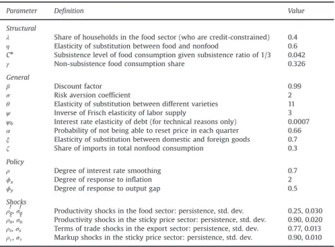
Parameter selection for the model is a challenging task. There is no consensus on the values of some parameters and those used in the literature are mostly based on micro data from advanced countries. We pick baseline parameters from the existing literature and then do extensive sensitivity analysis with respect to the choice of key parameters (Table 3).

The discount factor

β

equals 0.99, which amounts to an annual real interest rate of 4 percent. It is assumed that

λ

equals 0.4, implying that 40 percent of households in the economy are credit constrained, consistent with the data inTable 2. The baseline value of the risk aversion parameter

σ

¼2 is the value most commonly used in the literature on developing economies (Aguiar and Gopinath, 2007;Devereux et al., 2006;García-Cicco et al., 2010).

FollowingBasu and Fernald (1995)andBasu (1996), the parameter

θ

equals 11 (elasticity of substitution between the differentiated goods), implying a markup of 10 percent in the steady state. The probability that a price does not adjust in a given period (

α

) is set at 0.66 (Rotemberg and Woodford, 1997). This implies that prices remain fixed for a mean duration of three quarters, consistent with the microeconomic evidence for both developing and advanced economies.6_{The appropriate}

value of the Frisch elasticity (1=

ψ

) is both important and controversial. For our benchmark case it is assumed to be 0.33 (

ψ

¼3). For the monetary policy parameters, we followGalí et al. (2004)andMohanty and Klau (2005)and choose

ρ

¼0:7,

ϕ

π¼2, and

ϕ

y¼0:5.

An important feature of developing countries is the high share of food expenditure in total household expenditures. To calibrate the subsistence level food consumption parameterCn

and the weight on food in the consumption index

γ

, it is assumed that the average expenditure on food is around 42 percent (consistent with household surveys in developing countries). It is also assumed that on average one third of households' steady state food consumption is required for subsistence, enabling us to match estimates of the income elasticity of food consumption (about two-thirds).7 _{As the}

Table 3

Parameter values.

Parameter Definition Value

Structural

λ Share of households in the food sector (who are credit-constrained) 0.4 η Elasticity of substitution between food and nonfood 0.6 Cn

Subsistence level of food consumption given subsistence ratio of 1/3 0.042 γ Non-subsistence food consumption share 0.326

General

β Discount factor 0.99

σ Risk aversion coefficient 2

θ Elasticity of substitution between different varieties 11 ψ Inverse of Frisch elasticity of labor supply 3 ψb Interest rate elasticity of debt (for technical reasons only) 0.0007

α Probability of not being able to reset price in each quarter 0.66 ξ Elasticity of substitution between domestic and foreign goods 0.7 ζ Share of imports in total nonfood consumption 0.3

Policy

ρ Degree of interest rate smoothing 0.7

ϕπ Degree of response to inflation 2

ϕy Degree of response to output gap 0.5

Shocks ρa

f

,σa f

Productivity shocks in the food sector: persistence, std. dev. 0.25, 0.030 ρa

s

,σa s

Productivity shocks in the sticky price sector: persistence, std. dev. 0.90, 0.020 ρs,σs Terms of trade shocks in the export sector: persistence, std. dev. 0.77, 0.013

ρτ,στ Markup shocks in the sticky price sector: persistence, std. dev. 0.90, 0.010

6_{Evidence from Brazil (Gouvea, 2007), Chile (Medina et al., 2007), Mexico (Gagnon, 2009), and South Africa (Creamer and Rankin, 2008) indicates that} the frequency of price adjustment is much higher for food than for nonfood products and that price adjustments are less frequent during periods of low to moderate inflation. Since our model has no trend inflation and we impose price stickiness only in the nonfood sector, our parameter choice is consistent with the results of these studies.

demand for food is inelastic, we set

η

¼0:6 for the baseline case. Along with the subsistence level of food consumption, this implies a price elasticity of the demand for food of around 0.3 in the steady state, which is close to the USDA estimate. The major argument in favor of excluding food from the core price index is that the shocks to that sector are seasonal and transient. The value of the AR (1) coefficient of the food sector shock is set at 0.25 (implying that the shock has low persistence, which seems reasonable given the heavy dependence of agriculture on transitory weather conditions). Following the literature, the value of the AR(1) coefficient of the nonfood sector shock is set at 0.9 (Aguiar and Gopinath, 2007). The volatility of productivity shocks in developing countries is higher than in advanced countries (Pallage and Robe, 2003;García-Cicco et al., 2010). We set the standard deviation of the food productivity shock

σ

fa¼0:03 and the standard

deviation of the nonfood productivity shock

σ

s

a¼0:02. We followDevereux et al. (2006)in calibrating the persistence and

standard deviation of the terms of trade shock and choose

ρ

s¼0:77 and

σ

s¼0:013. We set the persistence of the mark-up

shock

ρ

τ¼0:9 and the standard deviation parameter

σ

τ¼0:01.

4. Baseline results

While it is not our objective to match specific moments, the incomplete markets version of our model more closely matches the properties of business cycle fluctuations in developing economies relative to advanced economies. For instance, with the baseline parameters and shock processes, the incomplete markets model delivers inflation that is more volatile than in the complete markets model. This is consistent with the empirical findings ofFraga et al. (2004);Bowdler (2005), andPétursson (2008)that developing economies have more volatile inflation than advanced ones.8_{In our model, the reason}

for this is that, due to lack of risk-sharing and consumption smoothing, the relative price between food and sticky price nonfood goods tends to be more volatile, rendering overall inflation also more volatile. Consumption is more volatile in the incomplete markets model, matching the findings ofAguiar and Gopinath (2007)andKose et al. (2009)that consumption is more volatile in developing economies than in advanced economies.

We now present the conditional welfare gains associated with different policy rules in our model. We include all four shocks–productivity shocks to two sectors, mark-up shocks, and terms of trade shocks– when conducting the welfare calculations discussed below.

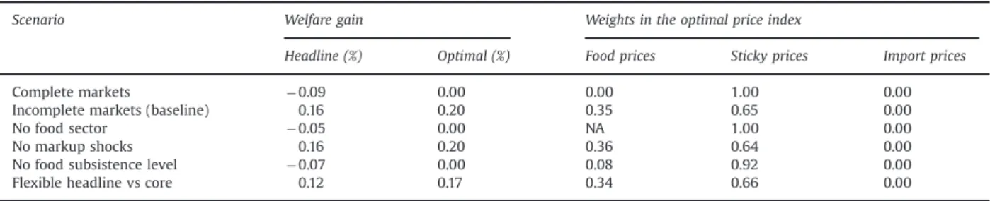
Table 4shows the welfare comparisons from targeting different price indices under complete and incomplete market settings, and also the sectoral weights for constructing the optimal price index in each case. With complete markets, the optimal price index puts the entire weight on the sticky price sector, with zero weights on food and traded goods, making it identical to core inflation targeting. Targeting headline inflation slightly reduces welfare. Thus, under complete markets, the choice of targeting strict core inflation is the best policy and dominates targeting of broader price indexes, as inAoki (2001)

andBenigno (2004).

However, with incomplete markets, this result no longer holds. The second row ofTable 4shows that headline inflation targeting is now welfare improving relative to core inflation targeting. Targeting the optimal price index yields a slightly higher welfare gain than targeting headline inflation.9_{The optimal price index assigns a weight of two-thirds to the sticky}

price sector and one-third to food prices. This result is a marked departure from the prior literature based on complete markets, wherein the optimal weight on food prices would be zero. On the other hand, it is consistent with theBenigno (2004)result (and, implicitly, the results of (Aoki, 2001) and (Mankiw and Reis, 2003) that the weight on the traded goods sector is zero. That sector has flexible prices and agents in that sector have access to financial markets, so the classical result is confirmed.

To investigate these results more carefully, we analyze the responses of key variables to a food productivity shock because shocks to that sector highlight the relevance of market completeness.Fig. 1plots the impulse responses of various macroeconomic variables to a one percent negative food productivity shock under complete markets. Each variable's response is expressed as the percentage deviation from its steady state level. Impulse responses under a strict core inflation targeting rule are shown by the solid lines. The dashed lines are impulse responses under a strict headline inflation targeting rule. The strict headline inflation targeting regime results in a slightly higher volatility of consumption and output. Also, the policy response is more aggressive under strict headline inflation targeting, which leads to a further decline in output. These results are similar to those documented in the existing literature on inflation targeting.

Following an increase in inflation, the central bank raises interest rates, reducing aggregate demand (as consumers postpone their consumption following an increase in interest rates) and, thus, inflation. So, under complete markets, stabilizing core inflation is equivalent to stabilizing the output gap (Aoki, 2001) and there are no additional welfare gains from adopting headline inflation targeting. Thus, core inflation targeting is the welfare maximizing policy choice for the central bank.

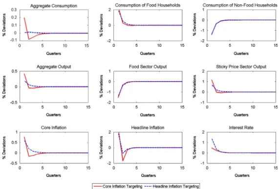
However, in the presence of credit constrained consumers, headline inflation targeting appears to be a better policy choice.Fig. 2plots the impulse responses of various macroeconomic variables to a one percent negative food productivity shock under incomplete markets. Aggregate demand responds differently to monetary tightening under strict core inflation

8_{Please refer to the online appendix for more details.}

targeting and headline inflation targeting. The central bank is now able to effectively control aggregate demand by increasing interest rates only when it targets headline inflation. Aggregate demand, instead of going up slightly, goes up sharply in response to the shock if the central bank follows strict core inflation targeting. Thus, headline inflation targeting outperforms core inflation targeting as the former is more effective at stabilizing output.

In order to examine the mechanics behind this result, we look at the properties of aggregate demand under incomplete markets. In the presence of financial frictions, the consumption choices of different households vary (as opposed to complete markets, where the consumption choice of each household is identical). While the consumption demand of unconstrained households is responsive to interest rates (as they optimize intertemporally), the consumption demand of credit-constrained households is independent of interest rate changes and depends only on their current period wage income. Since only a fraction of aggregate demand is influenced by interest rate changes, a monetary tightening does not automatically mitigate the increase in aggregate demand. The response of aggregate demand crucially depends on the behavior of credit-constrained households.

Fig. 2shows that, following a negative shock to food productivity, the central bank raises the interest rate, lowering the demand of unconstrained households (as it is optimal for them to postpone consumption). However, it has no bearing on the demand of credit-constrained consumers. An increase in the relative price of food following a negative food productivity shock increases the wage income and, therefore, consumption demand of credit-constrained households. Thus, the demand of the two types of households moves in opposite directions following a negative shock to food productivity.

Table 4

Welfare comparisons under different inflation targets.

Scenario Welfare gain Weights in the optimal price index

Headline (%) Optimal (%) Food prices Sticky prices Import prices

Complete markets 0.09 0.00 0.00 1.00 0.00

Incomplete markets (baseline) 0.16 0.20 0.35 0.65 0.00

No food sector 0.05 0.00 NA 1.00 0.00

No markup shocks 0.16 0.20 0.36 0.64 0.00

No food subsistence level 0.07 0.00 0.08 0.92 0.00

Flexible headline vs core 0.12 0.17 0.34 0.66 0.00

Notes: The optimal price index comprises food prices, sticky nonfood domestic goods prices, and import prices. Welfare gains under alternative inflation targets are derived as permanent consumption gains relative to strict core inflation targeting. The third, fourth, and fifth rows show results when we introduce one deviation at a time from the baseline incomplete markets model. The last row compares flexible headline inflation targeting versus flexible core inflation targeting, where both rules include a positive weight on the output gap.

Which of the two demands dominates is determined by the policy regime. Under core inflation targeting, the increase in food prices (and, therefore, the wage income of food sector households) is higher than under headline inflation targeting. This higher wage income translates into higher consumption demand by credit-constrained consumers (who consume all of their current wage income), more than compensating for the lower consumption demand of unconstrained consumers. Consequently, aggregate demand rises. By contrast, when the central bank targets headline inflation, price increases in the food sector are lower and the rise in income and, therefore, the increase in consumption demand in that sector is smaller. Thus, monetary intervention is effective in achieving its objective of controlling aggregate demand only when the central bank targets headline inflation.

To formalize the above arguments, we examine the log-linearized aggregate demand equation, which is given by10

^ ct¼

ð1

λ

Þ

ζ

s

σ

Et R^t

π

^tþ1

þEtc^tþ1

λζ

fEt

Δ

c^f;tþ1 ð20Þ

where

ζ

f¼Cf=Cis the steady state share of food sector households' consumption and

ζ

s¼Cs=Cis the steady state share of

nonfood sector households' consumption.

Furthermore, from the optimal labor supply of food sector households, we have

^ cf;t¼

1þa

ψ

1þa

σ

ψ

^ xf;tþ

a 1þ1

ψ

1þa

σ

ψ

^

Af;t ð21Þ

wherea¼xfyx=Cf41.

Eqs.(20) and (21) suggest that, in the presence of credit-constrained consumers, there is a link between aggregate demand and the relative price of foodðxf;tÞ. In this setting, relative prices affect aggregate demand in addition to aggregate supply. Thus,

the presence of financial frictions implies that managing aggregate demand requires the central bank to choose a policy regime that would limit the rise in wages of credit-constrained consumers (and, therefore, the increase in their demand).

We now present a series of variants of our benchmark model to investigate which features are quantitatively most important in driving our results. In the third row ofTable 4, we consider a model without a food sector. The economy now has one sticky price sector while import prices are flexible. Core inflation targeting is now better than headline inflation targeting (which would have a positive weight on import prices), confirming the classical result ofAoki (2001). The optimal

Fig. 2. Impulse responses to a negative food productivity shock (incomplete markets). Notes: The impulse responses shown above are to a one percent negative shock to food productivity. Each variable's response is expressed as the percentage deviation from its steady state level.

price index assigns a weight of zero to import prices, consistent withBenigno (2004)and indicating that openness of the economy is not crucial to our results.

In the fourth row ofTable 4, we consider a variant of the baseline model with no markup shocks. When the economy is only hit by productivity and terms of trade shocks, it is still the case that the welfare gains from targeting headline inflation rather than core inflation are positive. The parameters in the optimal price index are also almost identical to those in the baseline case. Thus, unlike in the complete markets setting ofMankiw and Reis (2003), we find that markup shocks do not matter greatly in determining the right price index to target.

In the fifth row ofTable 4, we evaluate the importance of the assumption of a subsistence level of food consumption. As noted earlier, this assumption affects the elasticity of substitution between food and nonfood goods. When we drop this assumption, targeting headline inflation leads to lower welfare than targeting core inflation. The intuition for this result is that, with perfect substitutability between food and nonfood, agents in the economy simply alter their consumption in response to a change in relative prices when there is a sector-specific productivity shock.

Thus, our main result is that the combination of incomplete financial markets and a subsistence level of food consumption, which are both characteristics relevant to developing economies, makes it optimal for an inflation-targeting central bank to target headline rather than core inflation.

Next, we evaluate more practical monetary policy rules employed even by inflation targeting central banks, which typically include the output gap. The results in the last row ofTable 4show that flexible headline inflation targeting delivers better welfare outcomes than flexible core inflation targeting. This is true whether the price index in headline inflation targeting is based on CPI weights or the optimal price index. The weight on food, nonfood, and imported goods in the optimal price index is essentially the same as under strict headline inflation targeting.

5. Sensitivity analysis and extensions

In this section, we report results from a variety of experiments to test the robustness of our results to changes in the values of key parameters and certain aspects of the structure of the model. Our results held up quite well to changes in values of most parameters, so in the discussion below we focus on the elements of our model that represent significant deviations from the prior literature. It should be noted that, since the steady state values of the models differ, it is only possible to make a comparison across regimes and not across different models.

5.1. Sensitivity to key parameters

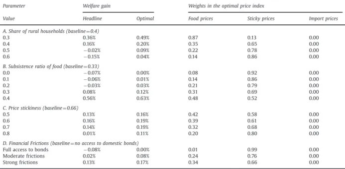
One of the key parameter settings in the model is the proportion of households in the economy that are in the food sector and face credit constraints. As the share of households in this sector rises, welfare gains from headline inflation or optimal inflation targeting decline relative to core inflation targeting (seeTable 5, Panel A). This might seem counter-intuitive as these households lack access to credit. The mechanism for this result is as follows. When the share of rural households is larger, under our parameter assumptions they will be poorer on average while the nonfood sector households will be richer. For a given drop in agricultural output, the relative price of food goes up by less when the consumption of food (above the subsistence level) by nonfood sector households is larger. When the share of rural households is small, the food consumption of households in the nonfood sector is also small in the steady state. Therefore, to accommodate a drop in food production, the relative price responds sharply.11

An important assumption in the model is the subsistence level of food. As noted earlier, this constraint does not bind in equilibrium but reduces the elasticity of substitution between food and nonfood goods. As shown inTable 4, when there is no subsistence level of food consumption, the weight of food in the optimal inflation target is small and core inflation targeting actually delivers higher welfare than headline inflation. As the subsistence level goes up, the weight of food in the optimal inflation index rises and core inflation targeting becomes inferior to headline inflation targeting (seeTable 5, Panel B). Note that in our model the total share of food consumption is pinned down based on empirical estimates for developing economies. A higher subsistence level of food therefore implies a lower level of nonsubsistence food consumption. Therefore, for any given amount of drop in the food output, market clearing necessitates a larger increase in the relative price of food. As a result, the higher is the subsistence level of food, the more volatile the impulse responses will be and the larger the welfare gain from headline inflation targeting.

An alternative approach to including a subsistence level of food in the utility function would be to directly pick a lower value for the elasticity of substitution between food and nonfood goods. Dropping the assumption that there is a subsistence level of food and lowering the elasticity to 0.38 yielded results similar to our baseline results. However, our approach is more realistic for developing economies. Empirical evidence shows that the income elasticity of food consumption is smaller than one in developing economies, which suggests it is more likely that food consumption is driven by the subsistence level.12

11_{Reducing the share of food sector households even further leads to implausibly large welfare gains, but this is because we have pinned down the} average share of food expenditures in total household expenditures to be 0.42. Economies with small shares of rural households tend to be richer economies with substantially lower food shares in total expenditure.

Another crucial parameter in the model is the share of food in total household consumption expenditures. When this share is small, the optimal inflation target puts most of the weight on the sticky price sector. Core inflation targeting then delivers higher welfare than headline inflation targeting, and the gains from targeting the optimal inflation index are modest. As the food share rises, the optimal inflation index involves an increasing weight on food prices. When food accounts for half of total consumption expenditures on average, the gains from headline inflation targeting become large and the optimal inflation index puts nearly the entire weight on food prices. This result appears at odds with one of the results inMankiw and Reis (2003). They find that“the more important a price is in the consumer price index, the less weight that sector's price should receive in the stability price index.”The incomplete markets structure of our model and the low elasticity of substitution between food and nonfood goods accounts for the difference between our result and theirs. However, our result that the weight on food prices is zero is true when markets are complete irrespective of the share of food in consumption expenditures, consistent with a different proposition in their paper–that sectors with more flexible prices should get a lower weight.

We also experimented with changing the degree of price rigidity in the sticky price sector (see Table 5, Panel C). Consistent withMankiw and Reis (2003)andBenigno (2004), the weight of the sticky price sector in the optimal price index increases with the degree of price stickiness. As the degree of price stickiness increases, the optimal price index converges to core inflation, so the gains from either headline or optimal inflation targeting (relative to core inflation targeting) start to fall when prices are highly rigid.

5.2. Financial frictions

In the baseline model, it is assumed that food sector households face strong financial frictions, turning them into hand-to-mouth consumers. We now relax this assumption by introducing a portfolio holding cost for these households, enabling us to vary the extent of (common) financial frictions they face (seeTable 5, Panel D). When the portfolio holding cost is zero, rural households have the same degree of access to the bond market as nonfood sector households. It is important to note that this is not equivalent to having complete financial markets. When the portfolio holding cost is very high, rural households hold zero bonds and the economy converges to the baseline incomplete markets case.

In the full access (but still not complete markets) scenario, food prices do enter with a nonzero weight in the optimal price index, although this weight is substantially smaller than in the baseline incomplete markets scenario. However, the welfare gain from targeting the optimal price index is small relative to core inflation targeting as the bonds give food sector households the ability to smooth consumption intertemporally although they cannot fully insure against sector-specific shocks. As the financial frictions become stronger, the welfare gains from headline inflation targeting rise and the share of food prices in the optimal price index also increases.

Table 5

Sensitivity tests.

Parameter Welfare gain Weights in the optimal price index

Value Headline Optimal Food prices Sticky prices Import prices

A. Share of rural households (baseline¼0.4)

0.3 0.36% 0.49% 0.87 0.13 0.00

0.4 0.16% 0.20% 0.35 0.65 0.00

0.5 0.02% 0.09% 0.22 0.78 0.00

0.6 0.15% 0.04% 0.14 0.86 0.00

B. Subsistence ratio of food (baseline¼0.33)

0.0 0.07% 0.00% 0.08 0.92 0.00

0.1 0.06% 0.01% 0.14 0.86 0.00

0.2 0.03% 0.03% 0.21 0.79 0.00

0.3 0.08% 0.12% 0.31 0.69 0.00

0.4 0.56% 0.63% 0.48 0.52 0.00

C. Price stickiness (baseline¼0.66)

0.5 0.13% 0.16% 0.42 0.58 0.00

0.6 0.16% 0.19% 0.39 0.61 0.00

0.7 0.14% 0.19% 0.32 0.68 0.00

0.8 0.01% 0.11% 0.20 0.80 0.00

D. Financial Frictions (baseline¼no access to domestic bonds)

Full access to bonds 0.08% 0.00% 0.01 0.99 0.00

Moderate frictions 0.02% 0.08% 0.24 0.76 0.00

Strong frictions 0.13% 0.17% 0.34 0.66 0.00

5.3. Common productivity shocks

Next, consider the case where there are only aggregate rather than sector-specific productivity shocks.13_{To this point, we}

have focused on the impact of a shock to productivity in the flexible price sector as it most clearly illustrates the point about what monetary policy rule is better in response to a shock to the flexible price part of the economy. Of course, while the impulse responses highlight different models' responses to only a food productivity shock, the simulation results include all shocks.

We recomputed the model with a productivity shock common to the food and the nonfood domestic goods sectors (and, as before, markup and terms of trade shocks as well). Intuitively, this should preserve the welfare gain from targeting inflation in the headline CPI or the optimal price index as there are no longer any shocks specific to the rigid price sector. This is indeed what we find, confirming our main results. The results go through whether the common productivity shock is transitory (food sector shock) or more persistent (sticky price sector shock). Besides, food prices consistently have a significant weight in the optimal inflation target.

5.4. Fiscal policy interventions

Since incomplete financial markets are important for driving our results, an important question from a policy perspective is whether other policy tools could be used to promote risk-sharing, improve welfare outcomes, and alter the relative merits of headline versus core inflation targeting. One obvious candidate is a state-dependent redistribution between households in the food and nonfood sectors through the tax and transfer system.

Consider, for instance, a food tax whose revenues are distributed across all households in a lump sum fashion. A food tax would lead to a larger redistribution from food sector households to other households when the economy is hit by a shock that drives up the price of food. This would result in a smaller change in the relative price of food compared to our baseline model. We conducted some numerical experiments showing that, as the food tax increased (up to a certain level), the economy approached the complete markets benchmark, with smaller gains from headline inflation targeting relative to core inflation targeting.14

In short, in lieu of headline inflation targeting, fiscal policy interventions can be used to complete markets and improve welfare in a developing economy with incomplete financial markets and a subsistence level of food consumption. Targeting transfers in this fashion might be challenging for a developing economy, due to political economy constraints and governance problems. Nevertheless, we recognize that this is an important topic for future research.

6. Concluding remarks

Previous research has concluded that optimal monetary policy should focus on offsetting nominal rigidities by stabilizing core inflation. However, those results rely on the assumption that markets are complete and that price stickiness is the only source of distortion in the economy. In this paper, we have developed a more realistic model for developing economies that has the following key features–incomplete markets with credit-constrained consumers; households requiring a minimum subsistence level of food; low price elasticity of the demand for food; and a high share of expenditure on food in households' total consumption expenditure. We nest models such as those of Aoki (2001)and Benigno (2004) as special cases of our model.

We show that the classical result about the optimality of core inflation targeting can be overturned by introducing financial frictions. In the presence of credit-constrained consumers, targeting core inflation no longer maximizes welfare. Moreover, stabilizing inflation is not sufficient to stabilize output when markets are not complete. Under these conditions, headline inflation targeting improves welfare. Our model also allows us to compute optimal price indexes that maximize welfare. The optimal price index includes a positive weight on food prices but, unlike headline inflation, generally assigns zero weight to import prices. This is because agents in that sector have access to financial markets and, unlike in the case of food, the price elasticity of the demand for goods produced in this sector is high.15_{A technical point to bear in mind is that,}

in the absence of aggregate homothetic preferences, it may no longer be optimal for monetary policy to target a particular price index. But our concern in this paper is about a practical choice that inflation targeting central banks face, which is typically to target an aggregate price index.

One possible extension of our model is to include money explicitly. While this provides a saving mechanism for hand-to-mouth consumers, it would also strengthen the case for headline inflation targeting to preserve the value of monetary savings. Another extension would be to explore how fiscal policy tools, such as food price subsidies that affect the relative price of food as well as specific state-contingent redistributive mechanisms, could be used to improve welfare even with

13_{Please refer to the online appendix for more details of the results discussed in this subsection and the next one.}

14_{We get the symmetric result that food price subsidies can increase relative price volatility and improve the benefits from headline rather than core} inflation targeting. The reason is that these subsidies would result in a net transfer from nonfood sector households to food sector households exactly when the relative price of food rises.

incomplete financial markets. In developing economies, such tools could be especially useful but are also more likely to be beset by problems in governance and implementation.

In future work, it will also be important to more explicitly consider the effects of particular inflation targeting rules on income distribution. For a normative analysis of optimal policies, distributional effects could be of first order importance in developing economies.16_{Another extension would be to include physical capital in the model. This highlights a practical}

dilemma that developing economy central banks often grapple with in pursuit of their objective of price stability. For instance, raising policy rates to deal with surging food price inflation can hurt industrial activity. While raising interest rates in response to a transitory negative shock to agricultural sector productivity might seem counter-intuitive, our results suggest that such a policy could in fact be welfare improving in an incomplete markets setting in which food consumption accounts for a large share of household consumption expenditures.

Acknowledgments

We are grateful to the editor, Ricardo Reis, and an anonymous referee for valuable comments. We also thank Kaushik Basu, Gita Gopinath, Karel Mertens, Parul Sharma, Viktor Tsyrennikov, and Magnus Saxegaard for helpful comments and discussions. We received helpful comments from seminar participants at the Bank of Korea, the Brookings Institution, Cornell University, the Federal Reserve Board, the IMF, and the Reserve Bank of India. We thank James Walsh for sharing some of his data with us. This research was supported by a grant from the International Growth Centre's Macroeconomics Program.

Appendix A. Supplementary data

Supplementary data associated with this article can be found in the online version athttp://dx.doi.org/10.1016/j.jmoneco. 2015.06.006.

References

Aguiar, M., Gopinath, G., 2007. Emerging market business cycles: the cycle is the trend. J. Polit. Econ. 115 (1), 69–102.

Anand, R., Prasad, E.S., 2010. Optimal price indices for targeting inflation under incomplete markets. NBER Working Paper No. 16290. Aoki, K., 2001. Optimal monetary policy responses to relative-price changes. J. Monet. Econ. 48 (1), 55–80.

Basu, P., Srivastava, P., 2005. Scaling-up microfinance for India's rural poor. World Bank Policy Research Working Paper No. 3646. Basu, S., 1996. Procyclical productivity: increasing returns or cyclical utilization?. Q. J. Econ. 111 (3), 719–751.

Basu, S., Fernald, J.G., 1995. Are apparent productive spillovers a figment of specification error? J. Monet. Econ. 36 (1), 165–188. Benigno, P., 2004. Optimal monetary policy in a currency area. J. Int. Econ. 63 (2), 293–320.

Bowdler, C., Malik, A., 2005. Openness and inflation volatility: panel data evidence. University of Oxford. Working paper. Calvo, G.A., 1983. Staggered prices in a utility-maximizing framework. J. Monet. Econ. 12 (3), 383–398.

Catão, L., Chang, R., 2010. World food prices and monetary policy. NBER Working Paper No. 16563.

Creamer, K., Rankin, N.A., 2008. Price setting in South Africa 2001–2007-stylised facts using consumer price micro data. Manuscript, University of the Witwaterstrand.

Demirguc-Kunt, A., Klapper, L., 2012. Measuring financial inclusion: the global findex database. World Bank Policy Research Working Paper No. 6025. Devereux, M.B., Lane, P.R., Xu, J., 2006. Exchange rates and monetary policy in emerging market economies. Econ. J. 116 (511), 478–506.

Erceg, C.J., Henderson, D.W., Levin, A.T., 2000. Optimal monetary policy with staggered wage and price contracts. J. Monet. Econ. 46 (2), 281–313. Ferrero, A., Gertler, M., Svensson, L.E., 2010. Current account dynamics and monetary policy. In: Galí, J., Gertler, M. (Eds.), International Dimensions of

Monetary Policy, University of Chicago Press, Chicago, IL, pp. 199–244.

Fraga, A., Goldfajn, I., Minella, A., 2004. Inflation targeting in emerging market economies. In: Gertler, M., Rogoff, K. (Eds.), NBER Macroeconomics Annual 2003, vol. 18. The MIT Press, Cambridge, MA, pp. 365–416.

Frankel, J.A., 2008. The effect of monetary policy on real commodity prices. In: Campbell, J.Y. (Ed.), Asset Prices and Monetary Policy, University of Chicago Press, Chicago, IL, pp. 291–333.

Gagnon, E., 2009. Price setting during low and high inflation: evidence from mexico. Q. J. Econ. 124 (3), 1221–1263.

Galí, J., López-Salido, J.D., Valles, J., 2004. Rule-of-thumb consumers and the design of interest rate rules. J. Money Credit Bank. 36 (4), 739–763. García-Cicco, J., Pancrazi, R., Uribe, M., 2010. Real business cycles in emerging countries? Am. Econ. Rev. 100 (5), 2510–2531.

Goodfriend, M., King, R., 1997. In: Bernanke, B.S., Rotemberg, J.J. (Eds.), The new neoclassical synthesis and the role of monetary policy, vol. 12. MIT Press, Cambridge, MA, pp. 231–296.

Goodfriend, M., King, R.G., 2001. The case for price stability. In: Herrero, A.G., Gaspar, V., Hoogduin, L., Morgan, J., Winkler, B. (Eds.), The First ECB Central Banking Conference: Why Price Stability? European Central Bank.

Gouvea, S., 2007. Price rigidity in Brazil: evidence from CPI micro data. Banco Central de Brasil Working Paper No. 143. Kose, M.A., Prasad, E.S., Terrones, M.E., 2009. Does financial globalization promote risk sharing? J. Dev. Econ. 89 (2), 258–270. Mankiw, N.G., Reis, R., 2003. What measure of inflation should a central bank target? J. Eur. Econ. Assoc. 1 (5), 1058–1086.

Medina, J.P., Rappoport, D., Soto, C., 2007. Dynamics of price adjustments: evidence from micro level data for chile. Central Bank of Chile Working Paper No. 432. Mishkin, F.S., 2007. Inflation dynamics. Int. Financ. 10 (3), 317–334.

Mishkin, F.S., 2008. Does stabilizing inflation contribute to stabilizing economic activity? NBER Working Paper No. 13970.

Mohanty, M.S., Klau, M., 2005. Monetary policy rules in emerging market economies: issues and evidence. In: Langhammer, R.J., de Souza, L.V. (Eds.), Monetary Policy and Macroeconomic Stabilization in Latin America, Springer, New York, pp. 205–245.

Pallage, S., Robe, M.A., 2003. On the welfare cost of economic fluctuations in developing countries. Int. Econ. Rev. 44 (2), 677–698. Pétursson, T.G., 2008. How Hard Can It Be? Inflation Control Around the World. Central Bank of Iceland, Economics Department.

Prasad, E.S., 2014. Distributional effects of macroeconomic policy choices in emerging market economies. IMF Econ. Rev. 62 (3), 409–429.

Rotemberg, J., Woodford, M., 1997. An optimization-based econometric framework for the evaluation of monetary policy. In: Bernanke, B.S., Rotemberg, J.J. (Eds.), NBER Macroeconomics Annual 1997, vol. 12, MIT Press, Cambridge, MA, pp. 297–361.

Schmitt-Grohé, S., Uribe, M., 2003. Closing small open economy models. J. Int. Econ. 61 (1), 163–185.

Schmitt-Grohé, S., Uribe, M., 2004. Solving dynamic general equilibrium models using a second-order approximation to the policy function. J. Econ. Dyn. Control 28 (4), 755–775.

Schmitt-Grohé, S., Uribe, M., 2007. Optimal simple and implementable monetary and fiscal rules. J. Monet. Econ. 54 (6), 1702–1725. Taylor, J.B., 1993. Discretion versus policy rules in practice. Carnegie–Rochester Conference Series on Public Policy, 39, pp. 195–214. Walsh, J.P., 2011. Reconsidering the role of food prices in inflation. IMF Working Paper No. 11/71.