Linear and Non-linear time series analysis: forecasting financial markets

(1)

“Linear and Non-Linear Time Series Analysis:

Forecasting Financial Markets”

Sandra Maria Mestre Barão

Dissertation submitted as partial requirement for the master’s degree in Prospection and Data Analysis

Supervisor:

Prof. Drª. Diana Aldea Mendes

(2)

ii Abstract

Time series analyses in financial area have been attract some special attention in the recent years. The stock markets are examples of systems with a complex behaviour and, sometimes, forecasting a financial time series can be a hard task. In this thesis we compare linear against non-linear models, ARIMA and Artificial Neural Networks. Using the log returns of nine countries we tried to demonstrate that neural networks can be used to uncover the non-linearity that exists in the financial field. First we followed a traditional approach by analysing the characteristics of the nine stock series and some typical features. We also produce a BDS test to investigate the nonlinearity, the results were as expected, and none of the markets exhibit a linear dependence. In consequence, traditional linear models may not produce reliable forecasts. However, this didn’t mean that neural networks can. We trained four types of neural networks for the nine stock markets and the results between them were quite similar varying most in their structure and suggesting that more studies about the hidden units between the input and output layer need to be done. This study stresses the importance of taking into account nonlinear effects that are quite evident in the stock market MODELS. JEL Classification: C32, C45, C53.

Keywords: Stock returns; Neural-Networks; ARIMA; Linear Time series; Non-Linear Time Series.

(3)

iii Resumo

A analise de séries temporais na area financeira tem atraido especial atenção nos últimos anos. Os mercados financeiros são exemplos de sistemas com um comportamento complexo e, por vezes, a previsão de séries temporais nesta àrea pode se tornar numa tarefa árdua. Nesta tese, iremos comparar os retornos logarítmicos proveninetes de nove mercados e monstrar que as redes neuronais podem ser utilizadas para detectar a não-linearidade existente nestes modelos. Primeiro, seguimos uma abordagem tradicional onde foram analisadas as características inerentes a cada um dos mercados. Executamos ainda o teste BDS para investigar a não-linearidade nas séries e, tal como esperado, os resultados confirmaram que nenhum dos mercados se apresenta como tendo um padrão linear. Dado este facto, os modelos lineares tradicionais poderão não produzir previsões fiáveis. Contudo, tal não quer dizer que as redes neuronais o façam. Foram treinadas quatro tipologias de redes para cada um dos nove mercados, sendo que, os resultados entre as mesmas foram bastante similares(variando em grande parte na estrutura que cada um das redes exibia) e, sugerindo que mais estudos devem ser feitos de modo a analisar o peso que as camadas ocultas possuem entre os neurónios de entrada e os de saída. Este estudo, enfatisa a importancia de se ter em conta que os efeitos não lineares devem ser estudados com certa significância nos mercados financeiros.

JEL Classification: C32, C45, C53.

Keywords: Retornos bolsistas; Redes-Neuronais, ARIMA; Séries Temporais Lineares; Séries Temporais não-lineares.

(4)

iv

Sumário Executivo

As séries temporais na área financeira têm atraído especial atenção nos últimos anos. Os mercados financeiros são exemplos de sistemas que apresentam um comportamento bastante complexo, na maioria dos casos, prever uma série financeira é muitas vezes uma tarefa considerada difícil. O estudo do comportamento dos valores dos mercados financeiros já existe à algum tempo e tem recebido uma permanente atenção ao longo das últimas décadas. Por exemplo em 1965, Fama, colocou ênfase na natureza estocastica do comportamento dos mercados financeiros e a partir daqui vários estudos seguiram com esta abordagem.

Esta tese pretende contribuir para uma melhor compreensão do problema relacionado com a previsão de variáveis provenientes de mercados financeiros. Para tal iremos procurar comparar modelos lineares (por exemplo, ARIMA) com modelos não lineares (Redes Neuronais) e perceber quais os modelos que obtêm uma maior performance/poder preditivo. Nesse sentido, iremos comparar a previsão de séries temporais, metodologia mais convencional e que se baseia em modelos de tendência/sazonalidade, com metodologias que assentam em modelos não lineares verificando qual dos métodos é o mais eficiente e em que condições, concretamente, quando tais modelos são aplicados a séries que não são muito bem comportadas.

A escolha do método ideal de previsão para uma determinada série não é um exercício simples, sendo que, uma revisão de literatura aponta que o aumento da complexidade das técnicas estáticas não implica um melhoramento da performance preditiva, ou a “accuracy”, muitas vezes os métodos considerados mais simples/tradicionais podem ser aplicados e apresentar uma performance superior. Gooijer e Hyndman (2006) referem que diversos autores apontam para a importância de que estudos futuros investiguem e definam as fronteiras em que Redes Neuronais Artificias e as técnicas tradicionais se superam umas em relação a outras.

Através de um conjunto de retornos logaritmicos provenientes de nove mercados (Portugal, Espanha, França, Alemanha, Itália, Grécia, Reino Unido, Japão, Estados Unidos) retirados através do DataStream.

Executamos ainda o teste BDS para investigar a não-linearidade nas séries e, tal como esperado, os resultados confirmaram que nenhum dos mercados se apresenta como tendo um padrão linear. Dado este facto, os modelos lineares tradicionais poderão não produzir previsões fiáveis. Contudo, tal não quer dizer que as redes neuronais o façam.

(5)

v

Foram treinadas quatro tipologias de redes para cada um dos nove mercados e os resultados entre si foram bastante similares, variando em grande parte na estrutura que cada um das redes exibia e sugerindo que mais estudos deveram ser feitos de modo a analisar o peso que as camadas ocultas entre os neurónios de entrada e os de saída.

Este estudo enfatisa a importância de se ter em conta que os efeitos não lineares devem ser estudados com certa significância nos mercados financeiros.

(6)

vi

Introduction

Time series an analysis in financial area has been attract some special attention in the recent years. The stock markets are examples of systems with a complex behaviour and, sometimes, forecasting a financial time series can be a hard task.

The study concerning the values from stock markets has been increasing in the last decades. For instance, in 1965, Fama launched the idea that stock markets had a stochastic behavior and from that period forward many studies follow this approach.

This thesis intends to contribute to a better understanding of the problem related to the stock market prediction. To accomplish this goal we will try to compare linear models (for instance, ARIMA models) with non-linear models (for instance, Artificial Neural Networks), namely, if the forecast and prediction power improves from one technique to other. Therefore, we will compare two kinds of forecasting time series analysis (a more conventional technique based on seasonal and trends models with a non-linear methodology) and check which of the methods is the most effective and under what conditions. Specially, when such model is applied to series that aren’t well behaved.

Empirical results show that Artificial Neural Networks (ANNs) can be more effectively used to make better forecasts than the traditional methods since stock markets have a complex structure are nonlinear, dynamic and even chaotic. Due to these reasons, ANNs can increase the forecast performance due to a learning process of the underlying relationship between de input and output variables and their ability to discover nonlinear relationships. Despite of all, ANNs also have some limitations, for instance, error functions of ANNs are usually complex, cumulative, and commonly they have many local minima, unlike the traditional methods. So, each time the network run with different weights and biases it arrives at a different solution. Many studies were been focused on the debate in the sense that the traditional approach in time series forecasting when applied in series with a well-behaviour can be more efficient but when applied in series that presents some noise and complexity (see, Enke, 2005, Ho et al., 2002) non-linear modelling techniques may overcome these problems. Enke (2005) refers that there is no evidence to support the assumption that the relationship between the stock returns and the financial variables is perfectly linear, due to the significant residual variance of the

(12)

2 stock return from the prediction of the regression equation. And, therefore, it is possible that nonlinear models (for instance, ANNs) are able to explain this residual variance and produce more reliable predictions.

Despite of all, the choice between one method and other is not an easy task. A literature review point out that the increasing complexity does not necessary increase the accuracy. Sometimes, the traditional statistics can be applied and present a higher performance. Gooijer and Hyndman (2006) refers that some authors stress the importance that future research needs to be done in order to define the frontiers were ANNs and the traditional methods can be more effective with a greater accuracy in relation to each other. For some tasks, neural networks will never replace traditional methods; but for a growing list of applications, the neural architecture will provide either an alternative or a complement to these other techniques. Our database consists in diary records from nine stock markets from different countries (Portugal, Spain, France, Germany, Italy, Greece, United Kingdom, Japan and United States of America) collected from the DataStream database. And it’s our main goal to study each of the techniques mentioned above for forecasting the same data and try to compare methodologies and verify in each situation which of them can be more efficient.

In terms of the structure of thesis, the Chapter 1 provides an introduction to the principal concepts of ARIMA and ANNs Models. This chapter gives an overview of the modelling techniques. Chapter 2 deals with the results and the modelling problem in these techniques. Finally, we will draw some conclusions about these two approaches, comparing the two methods and their results in our data. The software which we use was Clementine version 12.0.2 and Eviews version 6.

(13)

3

Chapter 1

1.1 Literature Review

1.1.1 Financial Time Series Analysis

Financial markets are complex dynamic systems with a high volatility and a great amount of noise. Due to these and other reasons we might say that forecasting financial time series can be a challenging task. In the past decades, strongest assumptions on financial time-series (namely the Random Walk Hypothesis) have been partially discharged.

Forecasting stock indexes involves an assumption that a primary source of information is available in the past and it has some predictive relationships to the future stock returns (Enke et al, 2005).

A time series is a sequence of variables whose values represent equally spaced observations of a phenomenon over time. We can write a time series as

{

x x1, 2,...,xt

}

or

{ }

xt , t = 1, 2,..., T (1.1)

where, we will treat x as a random variable. _t

The main objective of time series prediction can be stated as Ho et al. (2002) describes: “given a finite sequence x1, x2, x3 ,..., xt, find the continuation xt+1, xt+2”. The ability to predict time or at least the range within a specific confidence interval it is important in many knowledge areas for planning, decision making, etc, and time series analysis in financial area isn’t an exception.

A financial time series is said to be normal if its distribution is approximately similar to the bell-shaped theoretical distribution and linear if a model involving only first power on all the predictor variables can explain its underlying structure. Contrary to the established normality and linearity assumptions, research on stock prices finds the distribution is leptokurtotic (Brorsen and Yang 1994). Higher peaks relative to the normal distribution and fat tails characterize a leptokurtotic distribution.

Due to the fact that most of the current modeling techniques are based on linear assumptions there are emerging some authors that think that a non linear analysis of financial markets

(14)

4 needs to be considered. A technique that is emerging in this field is the use of neural networks, declared to be a universal approximator for nonlinear models.

1.1.2 Linear Time Series Analysis (ARIMA)

The classical linear regression model is the conventional starting point for time series and econometric methods. Peter Kennedy, in A Guide to Econometrics (1985), provides a convenient statement of the model in terms of five assumptions: (1) the dependent variable can be expressed as a linear function of a specific set of independent variables plus a disturbance term (error); (2) the expected value of the disturbance term is zero; (3) the disturbances have a constant variance and are uncorrelated; (4) the observations on the independent variable(s) can be considered fixed in repeated samples; and, (5) the number of observations exceeds the number of independent variables and there are no exact linear relationships between the independent variables.

While regression can serve as a point of departure for both time series and econometric models, it is incumbent on the analyst to generate the plots and statistics which will give some indication of whether the assumptions are being met in a particular context.

A time series model is a tool used to predict future values of a series by analyzing the relationship between the values observed in the series and the time of their occurrence. Time series models can be developed using a variety of time series statistical techniques. If there has been any trend and/or seasonal variation present in the data in the past then time series models can detect this variation, use this information in order to fit the historical data as closely as possible, and in doing so improve the precision of future forecasts.

There are many traditional techniques used in time series analysis. Some of these include:

■ Exponential Smoothing

■ Linear Time Series Regression and Curvefit ■ Autoregression

■ ARIMA (Autoregressive Integrated Moving Average) ■ Intervention Analysis

■ Seasonal Decomposition

In this thesis we’ll focus our analysis on ARIMA models. Until de 19th century, the study of time series was characterized by the idea of a deterministic world. Here, we can find the contribution of Yule (1927) which launched the notion of stochastic process in time series

(15)

5 analysis by postulating that every time series can be regarded as a realization of a stochastic process. Box and Jenkins in the 1970’s developed a coherent, versatile three-stage iterative cycle for time series identification, estimation and verification. Many of the ideas that have been incorporated into ARIMA models were by these authors (see Box et al, 1994), and for this reason ARIMA modelling is sometimes called Box-Jenkins modelling. ARIMA stands for AutoRegressive Integrated Moving Average, and the assumption of these models is that the variation accounted for in the series variable can be divided into three components:

■ Autoregressive (AR) ■ Integrated (I) or Difference ■ Moving Average (MA)

An ARIMA model can have any component, or combination of components, at both the nonseasonal and seasonal levels. There are many different types of ARIMA models and the general form of an ARIMA model is ARIMA(p,d,q)(P,D,Q), where:

■ p refers to the order of the nonseasonal autoregressive process incorporated into the

ARIMA model (and P the order of the seasonal autoregressive process)

■ d refers to the order of nonseasonal integration or differencing (and D the order of the

seasonal integration or differencing)

■ q refers to the order of the nonseasonal moving average process incorporated in the

model (and Q the order of the seasonal moving average process).

So for example an ARIMA(2,1,1) would be a nonseasonal ARIMA model where the order of the autoregressive component is 2, the order of integration or differencing is 1, and the order of the moving average component is also 1. ARIMA models need not have all three components. For example, an ARIMA(1,0,0) has an autoregressive component of order 1 but no difference or moving average component. Similarly, an ARIMA(0,0,2) has only a moving average component of order 2.

Autoregressive Models

In a similar way to regression, ARIMA models use independent variables to predict a dependent variable (the series variable). The name autoregressive implies that the series values from the past are used to predict the current series value. In other words, the autoregressive component of an ARIMA model uses the lagged values of the series variable, that is, values from previous time points, as predictors of the current value of the series

(16)

6 variable. For example, it might be the case that a good predictor of current monthly sales is the sales value from the previous month.

The order of autoregression refers to the time difference between the series variable and the lagged series variable used as a predictor. An AR(1) component of the ARIMA model is saying that the value of series variable in the previous period (t-1) is a good indictor and predictor of what the series will be now (at time period t). This pattern continues for higher-order processes.

The equation representation of a simple autoregressive model (AR(1)) is:

a

e

y

₍_t₎

=

Φ

₁ ₍_t₋₁₎

+

₍_t₎

+

(1.2)

Thus, the series value at the current time point (y(t)) is equal to the sum of: (1) the previous series value (y(t-1)) multiplied by a weight coefficient (Φ1); (2) a constant a (representing the series mean); and (3) an error component at the current time point (e(t)).

Moving Average Models

The autoregressive component of an ARIMA model uses lagged values of the series values as predictors. In contrast to this, the moving average component of the model uses lagged values of the model error as predictors.

Some analysts interpret moving average components as outside events or shocks to the system. That is, an unpredicted change in the environment occurs, which influences the current value in the series as well as future values. Thus the error component for the current time period relates to the series’ values in the future.

The order of the moving average component refers to the lag length between the error and the series variable. For example, if the series variable is influenced by the model’s error lagged one period, then this is a moving average process of order one and is sometimes called an MA(1) process, which can be expressed as:

a e e

y₍_t₎ =Φ₁* ₍_t₋₁₎ + ₍_t₎ + (1.3) Thus the series value at the current time point (y(t)) is equal to the sum of several components: (1) the previous time point’s model error (e(t-1)) multiplied by a weight coefficient (here Φ1); (2) a constant (representing the series mean); and (3) an error component at the current time point (e(t)).

(17)

7 Integration

The Integration (or Differencing) component of an ARIMA model provides a mean of accounting for trend within a time series model. Creating a differenced series involves subtracting the values of adjacent series values in order to evaluate the remaining component of the model. The trend removed by differencing is later built back into the forecasts by Integration (reversing the differencing operation). Differencing can be applied at the nonseasonal or seasonal level, and successive differencing, although relatively rare, can be applied. The form of a differenced series (nonseasonal) would be:

) 1 ( ) ( ) (t

=

y

t

−

y

t−

x

(1.4)

where the differenced series values (x(t)) is equal to the current series value (y(t)) minus the previous series value (y(t-1)).

Stationarity

In time series analysis the term stationarity is often used to describe how a particular time series variable changes over time. Stationarity has three components. First, the series has a constant mean, which implies that there is no tendency for the mean of the series to increase or decrease over time. Second, the variance of the series is assumed constant over time. Finally, any autocorrelation pattern is assumed constant throughout the series. For example, if there is an AR (2) pattern in the series; it is assumed to be present throughout the entire series. Any violation of stationarity creates estimation problems for ARIMA models. It is difficult to detect the true variations in the dependent variable if it is non-stationary. Because the mean of the series is changing over time, correlations and relationships between the variables in the ARIMA model will be exaggerated or distorted. Only if the mean of the dependent variable is stationary will true relationships and correlations be identified.

The Integration component of ARIMA is typically associated with removing trend from the series, which would violate the constant mean component of stationarity. It is often the case in time series analysis that the mean of a variable increases or decreases over time.

In order to make a series containing trend stationary, we can create a new series that is the difference of the original series. A first order difference creates a value for the new series which is the difference between the series value in the current period minus the series value in the previous period. Often the differenced series will have a stationary mean. If the

(18)

8 differenced series does not have a stationary mean then it might be necessary to take first differences of the differenced series. This transformation is known as second order differencing as the original series has now been differenced twice. The number of times a series needs to be differenced is known as the order of integration. Differencing can be performed at the seasonal (current time period value minus the value from one season ago) or non-seasonal (current time period minus the value from the previous time period) component. In short,

■ If a series is stationary then there is no need to difference the series and the order of

integration is zero. In all ARIMA models the dependent variable should be left in its original values. ARIMA models will be of the form ARIMA (p,0,q) where p is the order of the autoregressive process and q is the order of the moving average process in the model.

■ If a series is non-stationary then usually first differencing the series will make it

stationary. If first differencing makes the series stationary then the order of integration is one. ARIMA models will be in the form of ARIMA (p,1,q).

■ Very occasionally it might be necessary to difference a series twice to make it

stationary in which case the order of integration is two. It is however nearly always the case that first differences will make a non-stationary series stationary.

The Basic ARIMA Equation

Let Y* be the dependent series transformed to stationarity. Then the general form of the model is:

Y*t = φ1 Y*t-1 + φ2 Y*t-2 + … + φp Y*t-p + εt - θ1 * εt-1 – θ2 * εt-2 - … - θq *εt-q (1.5)

That is, Y* is predicted by its own past values along with current and past errors. The challenge with any dependent series is identifying the order of differencing and seasonal differencing, the order of autoregressive parameters, both nonseasonal and seasonal, and the order of moving average parameters, both nonseasonal and seasonal.

(19)

9 Identifying the Type of ARIMA Model

There are many different ARIMA models which could be fit to a particular time series of interest. The type of ARIMA model depends upon the selected orders of autoregression (p), integration (d), and moving average (q).

As with all times series analysis, we wish to find an ARIMA model that fits our financial historic data the closest and will perform the best when used for forecasting. In order to do this, it is necessary to select the optimal combination of p, d, and q. In other words, it is important to select the “right” combination of autoregressive, integration, and moving average orders. Unfortunately, it is often the case that identifying the p, d, and q combination to give the “best-fit or forecasting” ARIMA model is a process of trial and error. In many ways the identification stage is by far the most subjective in the entire ARIMA modelling process. The identification stage involves using exploratory techniques (sequence charts and autocorrelation and partial autocorrelation plots) in order to determine the most likely combination of p, d, and q that will give the closest fit to the historic data.

■ The order of integration (d) can usually be identified by looking at sequence charts for

the dependent variable (or the dependent variable after differencing).

■ Autocorrelation and partial autocorrelation plots of the dependent variable are used to

suggest plausible values for p and q, the orders of autoregression and moving average.

Identifying the Autoregressive (p) and Moving Average (q) Orders

The exploratory process for identifying the orders of autoregression and moving average is the subjective part of model identification. Identification of possible autoregressive (p) and moving average (q) orders requires examination of the autocorrelation and partial autocorrelation functions for the dependent variable. There are some theoretical guidelines of how autocorrelation and partial autocorrelation functions behave for different orders of autoregressive and moving average processes.

For instance, in a stationary model the ACF is {ρk : k ≥ 0}, where ρk is the correlation coefficient of Xt with Xt −k. Occasionally we will need to use ρ for k < 0. Remembering that ρ is an even function, so ρ −k = ρk. On the contrary, for a non-stationary model the ACF is undefined.

(20)

10 This suggests a technique for identifying a first-order MA, where we can see if the ACF is close to 0 except at lag 1. Checking whether a decrease is 'close to geometric' is much harder. The partial ACF (PACF) was introduced to combat this: the PACF of an AR(1) is 0 except at lag 1; the PACF of a MA(1) decreases geometrically.

The PACF is denoted by φk and defined to be the conditional correlation of Xt and Xt −k given all the values from t

−

k

+

1 to t −1, i.e. the extent of the relationship between Xt and Xt −k which is not accounted for by an AR(k −1) model.

To summarize, a pure autoregressive process is characterized by:

■ An exponentially or sine wave declining autocorrelation function

■ A number of spikes on the partial autocorrelation function equal to the order of the

(21)

11 1.1.3 Non-Linear Time Series Analysis (Artificial Neural Networks)

Detecting trends and patterns in financial data is of great interest to the business world to support the decision-making process. A new generation of methodologies, including neural networks, knowledge-based systems and genetic algorithms, has attracted attention for analysis of trends and patterns.

In particular, neural networks are being used extensively for financial forecasting with stock markets, foreign exchange trading, commodity future trading and bond yields. The application of neural networks in time series forecasting is based on the ability of neural networks to approximate nonlinear functions. In fact, neural networks offer a novel technique that doesn’t require a pre-specification during the modelling process because they independently learn the relationship inherent in the variables.

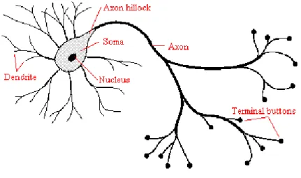
The term neural network applies to a loosely related family of model, characterized by a large parameter space and flexible structure, descending from studies such as the study of the brain function (see Figure 1). Neural nets have gone through two major development periods -the early 60’s and the mid 80’s. They were a key development in the field of machine learning. Artificial Neural Networks were inspired by biological findings relating to the behavior of the brain as a network of units called neurons. The human brain is estimated to have around 10 billion neurons each connected on average to 10.000 other neurons. Each neuron receives signals through synapses that control the effects of the signal on the neuron. These synaptic connections are believed to play a key role in the behaviour of the brain. The transmission of a signal from one neuron to another through synapses is a complex chemical process in which specific transmitter substances are released from the sending side of the junction. The effect is to raise or lower the electrical potential inside the body of the receiving cell.

McCulloch and Pitts (1943) developed computing machines designed to simulate the structure of the biological nervous system that could perform logic functions through learning. The neural networks can be a computer program or a hardwired machine that is design to learn in a manner quite similar to the human brain (Kutsurelis, 1998). Neural computing is an alternative to programmed computing which is a mathematical model inspired by biological models. This system is made up of a number of artificial neurons and a number of interconnections between them.

(22)

12 In a mathematical model a biological neuron is called perceptron. While in actual neurons the dendrite receives electrical signals from the axons of other neurons, in the perceptron these electrical signals are represented as numerical values. At the synapses between the dendrite and axons, electrical signals are modulated in various amounts. This is also modelled in the perceptron by multiplying each input value by a value called the weight.

Figure 1. Schematic of a Biological Neuron

However, the definition of a neural network, in fact, has varied as the field in which they are used. Due to this fact, we will consider the description given by Haykin (1998) that a neural network is a massively parallel distributed processor that has a natural propensity for storing experiential knowledge and making it available for use, resembling the human brain in two main respects:

■ The knowledge is acquired by a network through a learning process.

■ Interneuron connection strengths known as synaptic weights are used to store the

knowledge.

To differentiate a neural network from traditional statistical methods using this definition, for example, we may think that the traditional linear regression model can acquire knowledge through the least-squares method and store that knowledge in the regression coefficients. In this sense, it is a neural network. In fact, you can argue that linear regression is a special case of certain neural networks. However, linear regression has a rigid model structure and set of assumptions that are imposed before learning from the data. By contrast, the definition above makes minimal demands on model structure and assumptions. Thus, a neural network can

(23)

13 approximate a wide range of statistical models without requiring that you hypothesize in advance certain relationships between the dependent and independent variables. Instead, the form of the relationships is determined during the learning process. If a linear relationship between the dependent and independent variables is appropriate, the results of the neural network should closely approximate those of the linear regression model. If a nonlinear relationship is more appropriate, the neural network will automatically approximate the “correct” model structure. As Enke (2005) says neural networks offer the flexibility of numerous architecture types, learning algoritms and validation procedures.

The three basic components of the (artificial) neuron are:

1) The synapses or connecting links that provide weights, wj, to the input values, xj for j = 1,...m;

2) An adder that sums the weighted input values to compute the input to the activation function 1 m o j j j v w w x =

= +

∑

, where w0 is called the bias (not to be confused with statistical bias in prediction or estimation) and is a numerical value associated with the neuron. It is convenient to think of the bias as the weight for an input x0 whose value is always equal to one, so that

1 m j j j v w x = =

∑

;

3) An activation function g (also called a squashing function) that maps v to g(v) the output value of the neuron. This function is a monotone function.

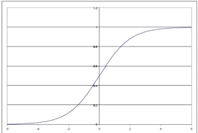
The activation function dampens or bound's the neuron's output. There are a large number of common activation functions in use with neural networks. Activation functions for the hidden units are needed to introduce nonlinearity into the network. Without nonlinearity, hidden units would not make nets more powerful than just plain perceptrons. The sigmoidal functions such as logistic and the Gaussian function (see Figure 2 and 3) are the most common choices.

When exists hidden units, the sigmoidal activation is preferable instead of the threshold activation functions. The lasts are difficult to train due do the error function (stepwise

(24)

14 constant) and the gradient or doesn’t exist or is equal to zero, making impossible to use backpropagation methods or becoming the gradient-based methods more efficient.

Figure 2. Logistic Function

Figure 3. Gaussian Function

eural etwork Architecture

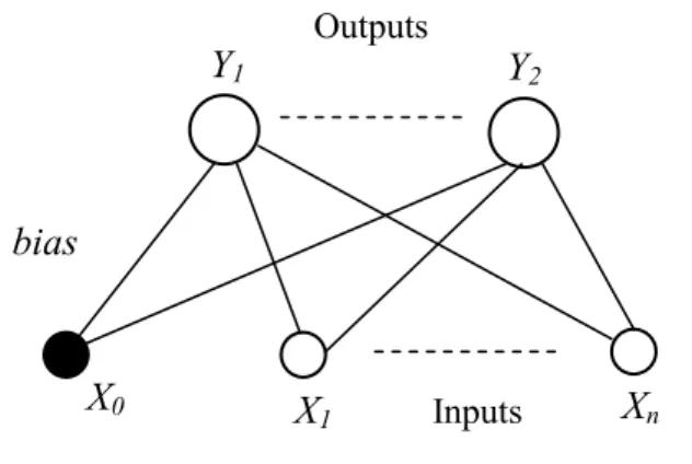
The simplest form of neural networks has two layers, an input layer and an output layer. The input layer consists of X0, X1,…, Xn variables and the output layer is also composed of many output variables such as Y0, Y1, …,Yn, where, each input (X) is linearly connected to each output (Y), defining a structure of the network (see for instance Figure 4).

(25)

15 Figure 4. Representation of a simplest neural network diagram.

In this Figure each component corresponds to a variable in the linear discriminant expression. The bias W0 can be considered as a weight parameter from an extra input whose activation X0 is permanently set to +1 (unity). We also can see that the Inputs X1, …, Xn are shown as circles, which are connected by the weights W1, …, Wn to the output Y. As in the human brain, the signals flow in one direction from the input to the output layer. The information flow is either activated or turned off depending on the value of the weights (or connection strengths). We can extend this representation to a set of multiple linear discriminant functions yk(x) as a neural network having a K output units.

Figure 5. Representation of neural network diagram with multiple linear discriminant functions.

The circles at the top of the diagram in Figure 5 corresponding to the functions yk(x) are sometimes called processing units, and the evaluation of the discriminant functions can be viewed as a flow of information from inputs to outputs. Each output yk(x) is associated with a weight vector Wk and a bias Wk0. We can express the network outputs in terms of the components of the vectors {Wk} and then mathematically, we have:

0 1 ( ) n k i i i Y X wk X wk = =

∑

+ (1.6) Output Y Inputs Xn X1 X0 Wn w1 W0 bias Outputs Inputs Xn X1 X0 Y2 Y1 bias

(26)

16 Then each line connecting an input i to an output k correspond to a weight parameter wki. As before, we can also regard the bias parameters as being weights from an extra input x0 = 1, to give 0 ( ) n k i i i Y X wk X = =

∑

(1.7)

Once the network is trained, a new vector is classified by applying it to the inputs of the network, computing the output unit activations and assigning the vector to the class whose output unit has the largest activation.

The more complex type of neural networks contains layers between inputs and outputs. This extra layer increases the learning capability of the model; and is known as a hidden layer. Being a connection between inputs and outputs the hidden layers creates an indirect relationship between them the information that is received in the input first is processed in the hidden layer and then transmitted to the output layer.

The learning technique is called the ‘Generalised Delta Rule’, which is basically error back propagation with the use of a momentum term. An example is then shown top the network, which is then propagated to the output yielding an answer. The difference between the answer and the target answer is the error. This error is fed backwards through the network and the weights updated by a factor of the error. This factor is referred to as η. Also a momentum term α is taken into account. The weight change is remembered and factored into to the next weight change. The control of the two learning parameters, η and α, is important in attempting to gain the best network.

According to the structure of the connections between the artificial neurons we can identify different classes of network architectures. The most common types of neural networks are the feedforward and the recurrent networks.

Figure 6. Example of a Feedforward Networks Diagram

X1

Inputs - X Hidden Layer

eurons - n Output - X X2 X3 n1 n2 Y

(27)

17

Figure 6 illustrates the architecture of a neural network with one hidden layer containing two neurons, three input variables {xi.} i = 1, 2, 3, and one output y. In addition to the sequential processing of typical linear systems, we can see parallel processing, in which only observed inputs are used to predict an observed output by weighting the input neurons, the two neurons in the hidden layer process the inputs in parallel fashion to improve predictions. The connectors between the input variables (input neurons) as well as the connectors between the hidden layers neurons and the output neuron are also called as synapses (linear activation function which connects to the one output layer with a weight on unity).

This single feedfoward or multiperceptron network with one hidden layer is the most basic and commonly used neural network in economic and financial applications (McNelis, 2005). Generally, the network represents the way the human brain processes input sensory data, received as input neurons into recognition as an output neuron. As the brain develops, more and more neurons are interconnected by more synapses, and the signals of the different neurons, working with parallel fashion, in more nuanced insight and reaction. In economic and financial applications, the combining of the input variables into various neurons in the hidden layers has an interesting interpretation, quite often we refer to latent variables, such as expectations, as important key drivers.

One typical method for training a network is to first partition the data series into three disjoint sets: the training set, the validation set and the test set. The network is trained directly on the training set, its generalization ability is monitored on the validation set, and its ability to forecast is measured on the test set.

A network that produces high forecasting error on unforeseen inputs, but low error on training inputs, is said to have overfit the training data. Overfitting occurs when the network is blindly trained to a minimum in the total squared error based on the training set. A network that has overfit the training data is said to have poor generalization ability.

(28)

18

Chapter 2

Forecasting Financial Markets

2.1 Methodology

For the current research our main objective was to compare traditional forecasting methods with the use of neural networks and then verify if the prediction power improves from one technique to other.

The following questions allow the research to meet the objectives proposed:

- What are the similarities and the differences between neural networks and the traditional methods such as ARIMA?

- Can neural networks accurately forecast financial markets?

- Can neural networks have a greater prediction power than traditional methods? In which situations?

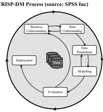
To create and test our models we used in major the software Clementine version 12.0. The choice of the software determined also our methodology or we can say also the key drivers to support our research. As with the most business endeavors and in the research field also, the data mining process is much more effective if done in a planned systematic way. Even with data-mining tools such as Clementine, the majority of work requires the careful eye of a knowledgeable business analyst to keep the process on track. And, to stay on track it helps if we have an explicitly defined process model. The data mining process model recommend for the use with Clementine is the Cross-Industry Standard Process for Data Mining (CRISP – DM) this model is designed as a general model that can be applied to a wide variety of industries and business problems.

The general CRISP-DM process model includes six phases (see Figure 8) that address the main issues in data mining. The six phases fit together in a cyclical process. These six phases

(29)

19 cover the full data mining process, including how to incorporate data mining into your larger business practices. The six phases include:

• Business understanding. This is perhaps the most important phase of data mining. Business understanding includes determining business objectives, assessing the situation, determining data mining goals, and producing a project plan. In our case, the business understanding corresponds to the gathering of the theoretical framework (literature review)

• Data understanding. Data provides the "raw materials" of data mining. This phase addresses the need to understand what your data resources are and the characteristics of those resources. It includes collecting initial data, describing data, exploring data, and verifying data quality.

• Data preparation. After cataloguing your data resources, you will need to prepare your data for mining. Preparations include selecting, cleaning, constructing, integrating, and formatting data.

• Modeling. This is, of course, the flashy part of data mining, where sophisticated analysis methods are used to extract information from the data. This phase involves selecting modelling techniques, generating test designs, and building and assessing models.

• Evaluation. Once you have chosen your models, you are ready to evaluate how the data mining results can help you to achieve your business objectives. Elements of this phase include evaluating results, reviewing the data mining process, and determining the next steps.

• Deployment. Now that you've invested all of this effort, it's time to reap the benefits. This phase focuses on integrating your new knowledge into your everyday business processes to solve your original business problem. This phase includes plan deployment, monitoring and maintenance, producing a final report, and reviewing the project.

There are some key points to this process model. First, while there is a general tendency for the process to flow through the steps in the order outlined above, there are also a number of places where the phases influence each other in a nonlinear way. For example, data preparation usually precedes modelling. However, decisions made and information gathered

(30)

20 during the modelling phase can often lead you to rethink parts of the data preparation phase, which can then present new modelling issues, and so on.

The second key point is the iterative nature of data mining. We will rarely, if ever, simply plan a data mining project. The knowledge gained from one cycle of data mining will almost invariably lead to new questions, new issues, and new opportunities to identify and meet your customers' needs. Those new questions, issues, and opportunities can usually be addressed by mining our data once again.

Figure 8. Stages in CRISP-DM Process (source: SPSS Inc)

Data Understanding Data Preparation Modelling Data Data Data Business Understanding Deployment Evaluation

2.2 Data Understanding and Data Preparation

To accomplish our goals the inputs to the models developed was obtained from the DataStream (http://www.datastream.com) that consists in diary records from nine stock markets from different countries: Portugal (TOTMKPT(PI)), Spain (TOTMKES(PI)), France (TOTMKFR(PI)),Germany(TOTMKBD(PI)),Italy(TOTMKIT(PI)),Greece (TOTMKGR(PI)), United Kingdom (TOTMKUK(PI)), Japan(TOTMKJP(PI)) and United States of America (TOTMKUS(PI)). Notice that we didn’t try to adjust our series to the same time frame. For instance our longest series is the UK series with 11161 records starting from 01-01-1965; and, the shortest is from Portugal series with 4639 records starting from 02-01-1990.

(31)

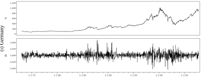
21 The first step has to perform a preliminary analysis on all the nine stock markets. For our analysis we used the log returns from these markets. The use of this variable has several advantages. For instance, it is additive, the return of the entire series is the sum of the returns comprising the series; when used in the correlation analysis, the log returns eliminate one trivial source of non-stationarity of the correlation functions. The next figures shows the original records series Pt and the corresponding logarithmic returns measured in percentage terms, denoted yt and computed as

(

1

)

100.

t t t

y = p −p₋ (2.1)

wherep_t =ln( )P_t .

Figure 9. Daily observations on the upper panel and returns on the lower panel of: (a) USA (b) Italy (c) Greece (d) Spain (e) Portugal (f) France (g) Japan (h) UK (i) Germany.

(a

)

U

S

(32)

22 (b ) It al y (c ) G re ec e (d ) S p ai n

(33)

23 (e ) P o rt u g al

(34)

24 (f ) F ra n ce (g ) Ja p an (h ) U K

(35)

25 The summary statistics for the stock returns are given in Table 1 for daily sampling frequencies. Theses statistics are used in the discussion of the characteristics features of these series.

One of the assumptions in the finance literature is that the logarithmic returns yt are normally distributed variables, with mean µ and variance δ2, that is,

_(2.2)

Table 1. Summary statistics for stock returns

Stock Market Records Mean Med S.D. Min Max Var Skew Kurt Jarque-Bera Sig.

Daily returns USA 9073 0.0003 0.0002 0.0097 -0.2071 0.0835 0.0001 -1.1532 26.9002 275254.3 0.000 Italy 9074 0.0004 0.0001 0.0130 -0.0984 0.0918 0.0002 -0.2902 4.9407 9343.829 0.000 Greece 5159 0.0006 0.0000 0.0166 -0.1463 0.1531 0.0003 0.0201 8.3338 14896.75 0.000 Spain 5379 0.0003 0.0003 0.0112 -0.0947 0.0741 0.0001 -0.3997 5.3366 6511.575 0.000 Portugal 4638 0.0002 0.0000 0.0085 -0.0801 0.0627 0.0001 -0.4558 8.5523 14260.27 0.000 France 9074 0.0365 0.0161 1.1218 -9.8948 7.9666 1.2584 -0.3575 4.9019 9265.549 0.000 Japan 9074 0.0002 0.0000 0.0102 -0.1574 0.0939 0.0001 -0.3697 11.7629 52457.25 0.000 UK 11160 0.0003 0.0000 0.1717 -1.1165 1.1059 0.0295 0.0666 6.9477 22430.54 0.000 Germany 9074 0.0002 0.0002 0.0098 -0.1214 0.0591 0.0001 -0.6626 8.0390 25066.76 0.000

The kurtosis of yt is defined as

(i ) G er m an y

(36)

26

(

)

4 4 t y y K = E − µ _ σ   (2.3)

The kurtosis for normal distributions is equal to three. One of the characteristics that we can observe from the Table 1 is that the kurtosis of all the series is much larger than this normal value. This reflects that the tails of these series are fatter than the tails of the normal distribution. This is also called the fat tail phenomenon (excess kurtosis), time series that exhibit a fat tail are often called leptokurtic. USA presents the highest excess of kurtosis followed by Japan, where the presence of excess of kurtosis is more notorious.

Except in UK and Greece it is possible to observe presence of negative asymmetry, all symmetric distributions have skewness equal to zero.

The skewness of yt is defined as

(

)

3 3 t y y SK = E − µ _ σ   (2.4)

As we can see most of the stock return series have negative skewness, implying that the left tail of the distribution is fatter that the right. Finally, and given the skewness and kurtosis results, the Jarque-Bera test rejects the null hypothesis that the data are from a normal distribution for all the series.

The Jarque-Bera test of yt is defined as

( )2 2 6 ₄ n _k JB= __s ₊ − 3 _   (2.5)

where n is the number of observations (or degrees of freedom in general); S is the sample skewness, K is the sample kurtosis.

As we can see, these results are consistent with the series distributions in financial time series analysis.

A frequent problem with economic and financial data is that it is manifestly nonstationary. The econometric consequences of nonstationary time series are very severe, in that estimators and t-statistics are unreliable. Nonstationary time series do not exhibit constant means and variances. As we can see from the Figure 9 above representing the nine stock markets, these series varies over time, and it is and indication that the mean and variance are not constant. One reason macroeconomists got interested in unit roots is the question of how to represent trends in time series. The unit root test has recently become popular in econometrics as a test for stationarity; the presence of a unit root causes the autocorrelations to be varying over time and invalidates their use for specification of the appropriate AR order.

(37)

27 In this context, we applied the unit root test, with the goal to determine the integration order of a given series (and their stationarity). Dickey and Fuller (1979) and Fuller (1976) developed a basic test for unit root and order of integration, testing the statistical relevance of yt-1 in the auxiliary regression. The null hypothesis is ρ = 0 and the alternative is ρ < 0, resulting in a one-sided test. The distribution is nonstandard because under the null hypothesis of a unit root, the yt series is nonstationary.

The Augmented DF statistics (see the appendix B) are larger in absolute values than the critical values; so we rejected the hypothesis of nonstationarity. We therefore conclude that the daily log return of the nine series is stationary.

(38)

28 2.3 Modeling

2.3.1 ARIMA - Modeling Results

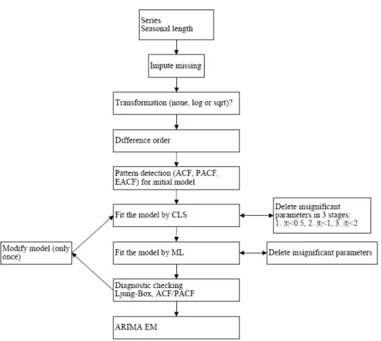
After doing some exploratory analysis to the data series, we worked with Clementine Expert Modelling – Time Series Analysis in order to determine the best ARIMA model for all the nine series. The ARIMA Expert Model has the following structure:

Figure 10. ARIMA Model Detection

Through this procedure we applied the Box-Jenking methodology and in the step related to the pattern detection for initial model (Autocorrelation Function (ACF) and Partial Auto Correlation Coefficient (PACF), we determined the adequate ARIMA model (p,d,q)(P,D,Q) incorporating both seasonal and nonseasonal levels.

The Box Jenkins modelling procedure consists of three stages; identification, estimation and diagnostic checking. (1) At the identification stage a set of tools are provided to help identify a possible ARIMA model, which may be an adequate description of the data. (2) Estimation is simply the process of estimating this model. (3) Diagnostic checking is the process of

(39)

29 checking the adequacy of this model against a range of criteria and possibly returning to the identification stage to respecify the model. The distinguishing stage of this methodology is identification.

This approach tries to identify an appropriate ARIMA specification. It is not generally possible to specify a high order ARIMA model and then proceed to simplify it as such a model will not be identified and so can not be estimated. The first stage of the identification process is to determine the order of differencing which is needed to produce a stationary data series. The next stage of the identification process is to assess the appropriate ARMA specification of the stationary series.

For a pure autoregressive process of lag p, the partial autocorrelation function up to lag p will be the autoregressive coefficients while beyond that lag we expect them all to be zero. So in general there will be a ‘cut of’ at lag p in the partial autocorrelation function. The correlogram on the other hand will decline asymptotically towards zero and not exhibit any discreet ‘cut of’ point. An MA process of order q, on the other hand, will exhibit the reverse property.

Table 2. Model ARIMA Summary (nine stock markets)

Model StationaryR2 R2 RMSE MAPE MAE MaxAPE MaxAENorm. BIC Q df Sig.

USA ARIMA(2,0,1)(1,0,1) 0.007 0.007 0.010 126.639 0.007 17770.006 0.205 -9.263 18.825 13 0.129 Italy ARIMA(0,0,4)(0,0,0) 0.020 0.020 0.013 196.235 0.009 88233.626 0.094 -8.707 43.794 16 0.000 Greece ARIMA(0,0,1)(0,0,0) 0.021 0.021 0.016 175.047 0.011 52805.306 0.152 -8.212 29.217 17 0.033 Spain ARIMA(0,0,1)(0,0,0) 0.008 0.008 0.011 119.294 0.008 19573.918 0.093 -8.988 31.500 17 0.017 Portugal ARIMA(1,0,4)(0,0,0) 0.022 0.022 0.008 122.881 0.006 6447.939 0.073 -9.569 39.351 16 0.001 France ARIMA(0,0,1)(0,0,0) 0.010 0.010 1.117 154.641 0.791 58094.263 10.185 0.223 36.766 17 0.004 Japan ARIMA(0,0,2)(1,0,1) 0.009 0.009 0.010 129.946 0.007 9332.552 0.156 -9.167 37.867 14 0.001 UK ARIMA(1,1,2)(0,0,0) 0.423 0.376 0.136 7450.358 0.086 6689035.455 1.067 -3.991 28.148 16 0.030 Germany ARIMA(0,0,4)(1,0,1) 0.006 0.006 0.010 118.894 0.007 10607.999 0.121 -9.250 36.525 14 0.001

Note: Q is the Ljung-Box Q statistic

To compare the linear predictability of the markets for daily observations, we use the following procedure. For each one of the markets and at any moment of time we consider the last 30 observations, and then we estimate autoregressive linear models.

Box and Jenkins (1970) showed that given a model adequacy, the population were uncorrelated and the variances were approximately equal to n-1. The Ljung-Box statistics can be used for this purpose. Under the null hypothesis of no residual autocorrelation at lag 1 to m in the residuals from an ARMA (p,q) model. As observed in Table 2, the USA series is the only that do not reject the null hypothesis about residual autocorrelation. As we can see from these results, these models have two drawbacks, in first the errors in the model may be

(40)

30 autocorrelated and second is that the variance of the error terms may not be constant over time. However, some authors refers the importance to investigate the robustness of the Q test in situations were the performance of the same may be influenced by the fatness of distributional tails (see Jansen and de Vries, 1991; Loretan, 1994). Simulations results showed that distributional heavy-tails may distort the asymptotic null distributions of the Q and reduce the power of these tests (see also, Franses and Van Dijk, 2000). Further, these tests can reject their null hypotheses due to nonlinearity or conditionally heteroskedastic skewness. By consequence, this topic brings us to the discussion about the assumption of linearity. And when this assumption is false many the basic results still hold. To test the hypothesis of non-linearity we used the Brock, Dechert, Scheinkman and LeBaron (1996) test, also called, BDS test. This test is unique in its ability to detect nonlinearities independently of linear dependencies in data. It rests on the correlation integral, developed to distinguish between chaotic deterministic systems and stochastic systems. The procedure consists of taking a series of m-dimensional vectors from a time series, at time t = 1, 2,…, T – m, where T is the length of the time series. The BDS statistics tests the difference between the correlation integral of embedding dimension m, and the integral for embedding dimension 1, raised to the power m (Mcnelis, 2005).

Table 3. BDS statistics

BDS Statistic Std. Error z-Statistic

2 3 4 5 6 2 3 4 5 6 2 3 4 5 6 USA 0.013 0.028 0.039 0.046 0.05 9E-04 0.001 0.002 0.002 0.002 13.8744 18.862 22.090225.1149 28.334 Italy 0.02 0.041 0.057 0.066 0.07 1E-03 0.002 0.002 0.002 0.002 21.413527.4396 31.71635.1357 38.747 Greece 0.033 0.067 0.09 0.105 0.113 0.001 0.002 0.003 0.003 0.003 23.554629.4441 33.542337.492141.7758 Spain 0.02 0.044 0.064 0.076 0.082 0.001 0.002 0.002 0.002 0.002 16.2971 22.426 27.180530.920134.6973 Portugal 0.028 0.054 0.074 0.086 0.092 0.001 0.002 0.003 0.003 0.003 18.8483 23.265 26.623929.912833.2719 France 0.018 0.036 0.05 0.057 0.06 9E-04 0.001 0.002 0.002 0.002 18.97624.5023 28.561631.569934.4414 Japan 0.021 0.045 0.065 0.078 0.084 0.001 0.002 0.002 0.002 0.002 20.505727.6293 33.239838.133542.8872 UK 0.061 0.117 0.159 0.186 0.203 0.001 0.002 0.002 0.002 0.002 48.896658.8725 66.678574.676284.1214 Germany 0.022 0.047 0.067 0.079 0.085 1E-03 0.002 0.002 0.002 0.002 22.939330.7445 36.588341.514746.3666 *The probability values are all significant for all the nine stock markets at the 0.00 (< 0.05).

The results of the BDS test shows that in all the nine stock markets returns exists a non-linear dependence. As a conclusion of this preliminary analysis, we can say that there exists statistical evidence in favour of a nonlinear structure in each of the daily series.

(41)

31 2.3.2 Artificial Neural Networks - Modeling Results

In this case, we employ ANNs to forecast next day returns. One of the main reasons that neural networks were in the past decades increased popularity is due to the fact that these models have been shown to be able to approximate almost any nonlinear function. Thus, when applied to series which is characterized by nonlinear relationships, neural networks can detect these and provide a superior fit compared to linear or even non-linear traditional models.

The neural networks used in this analysis are feed-forward multi layer perceptrons which employ a sigmoid transfer function. We analyzed the results of four feed-forward (known as multilayer perceptrons) neural networks:

(1) Quick method: when the quick method is selected; a single neural network is trained. By default, the network has one hidden layer containing max(3(n_i+n_o) / 20 neurons, where ni is the number of input neurons and no is the number of output neurons;

(2) Dynamic method: the topology of the network changes during training, with neurons added to improve performance until the network achieves the desired accuracy. There are two stages to dynamic training: finding the topology and training the final network; (3) Multiple method: multiple networks are trained in pseudo parallel fashion. Each specified network is initialized, and all networks are trained. When the stopping criterion is met for all networks, the network with the highest accuracy is returned as the final model. That is, at the end of training, the model with the lowest RMS error is presented as the final model;

(4) Prune method: that is, conceptually, the opposite of the dynamic method. Rather than starting with a small network and building it up, the prune method starts with a large network and gradually prunes it by removing unhelpful neurons from the input and hidden layers. Pruning proceeds in two stages: pruning the hidden neurons and pruning the input neurons. Pruning is carried out after a while if there is no improvement. Before initially pruning, or after any pruning, the network will run for a number of cycles, specified by the Persistence.

As we know, to training a neural network it is important to incorporate input neurons. Several studies showed that in econometric application it is common to use the p lagged variables directly as linear regressors.

(42)

32 0 1 0 1 1 2 2 0 1 2 1 ' ( ' ) ... ( , 1, 2, ... , ) q t t j t j j t t p t p q j j t j t j t p j y x G x i y y y G j y y p y i φ φ φ φ φ φ = − − − − − − = = + + β γ + ε = + + + + + β γ + γ + γ + + γ + ε

∑

(2.6)

The performance alternative models were evaluated with about 30% of all the data records in each series, evaluating how well competing models generalize outside of the data set used for estimation. This option was also taken due to the over training. To prevent the over training it’s useful to train the network with two sets: training and validation, and accuracy is estimated based on the validation set.

The performance simulations showed that in the major cases the quick and multiple neural

networks outperform better than the others as we can see from Table 4.

Table 4. Accuracy results from the four neural networks in the nine stock markets.

Accuracy HL (1) HL (2) Accuracy HL (1) HL (2) USA Quick 97.69 3 France Quick 97.16 3 Dynamic 97.66 2 Dynamic 97.19 2 2 Multiple 97.68 19 Multiple 97.2 19 10 Prune 97.67 3 Prune 97.19 2 Italy Quick 95.33 3 Japan Quick 97.27 3 Dynamic 95.22 2 2 Dynamic 97.25 2 2 Multiple 95.31 12 2 Multiple 97.31 19 Prune 95.29 4 Prune 97.31 9 Greece Quick 96.45 3 UK Quick 96.14 3 Dynamic 96.41 2 Dynamic 96.07 2 2 Multiple 96.43 . 10 Multiple 96,17 2 Prune 97.67 3 Prune 96.07 4 2 Spain Quick 95.39 3 Germany Quick 96.27 2 2 Dynamic 95.36 2 2 Dynamic 96.28 3 Multiple 95.39 12 Multiple 96.3 4 Prune 95.31 2 Prune 96.26 5 Portugal Quick 95.95 3 Dynamic 96.03 2 2 Multiple 95.95 19 Prune 96.23 2

(43)

33 Hornik et all. (1989) have demonstrated that, with a sufficient number of hidden layers, a neural network can approximate any given functional form to a desired accuracy level. In future studies it will be important to determine if the number of hidden layers may influence the accuracy results in data series and in what level. The hidden layer(s) provide the network with its ability to generalize. In practice, neural networks with one and occasionally two hidden layers are widely used and have performed very well. Increasing the number of hidden layers also increases computation time and the danger of overfitting which leads to poor out-of-sample forecasting performance.

Below we present for each of the nine series the two neural network architectures that achieved the best accuracy results.

Figure 11. The two “best accuracy” neural networks. Test data visualization. Where rt is the log return of the series and n-rt is the forecasted data.

USA (Quick Method) – Testing Data

(44)

34 Italy (Quick Method) – Testing Data

Italy (Multiple Method) – Testing Data

(45)

35 Greece (Prune Method) – Testing Data

Spain (Quick Method) – Testing Data

(46)

36 Portugal (Quick Method) – Testing Data

Portugal (Multiple Method) – Testing Data

(47)

37 France (Multiple Method) – Testing Data

Japan (Multiple Method) – Testing Data

(48)

38 UK (Quick Method) – Testing Data

UK (Multiple Method) – Testing Data

Linear and Non-linear time series analysis: forecasting financial markets