FUNDAÇÃO GETULIO VARGAS
ESCOLA DE ECONOMIA DE EMPRESAS DE SÃO PAULO
JOÃO MIGUEL SANCHES DE ANDRADE PISSARRA
TREND FOLLOWING PERFORMANCE WITH SIZE AND LIQUIDITY:
EVIDENCE FROM US, BRAZIL AND PORTUGAL
SÃO PAULO
2
JOÃO MIGUEL SANCHES DE ANDRADE PISSARRA
TREND FOLLOWING PERFORMANCE WITH SIZE AND LIQUIDITY: EVIDENCE FROM US, BRAZIL AND PORTUGAL
Thesis presented to Escola de Economia de Empresas de São Paulo of Fundação Getulio Vargas, as a requirement to obtain the title of Master in Finance.
Knowledge Field: International Master in Finance.
Adviser: Prof. Dr. João Mergulhão Prof. Dr. André Silva
SÃO PAULO
3
Pissarra, João.
Trend Following Performance with Size and Liquidity: Evidence from the US, Brazil and Portugal / João Pissarra. - 2014.
60 f.
Orientador: João Mergulhão, André Silva
Dissertação (MPFE) - Escola de Economia de São Paulo.
1. Ações (Finanças). 2. Investimentos. 3. Bolsa de Valores. 4. Mercado de capitais. I. João Mergulhão, André Silva. II. Dissertação (MPFE) - Escola de Economia de São Paulo. III. Título.
4
JOÃO MIGUEL SANCHES DE ANDRADE PISSARRA
TREND FOLLOWING PERFORMANCE WITH SIZE AND LIQUIDITY:
EVIDENCE FROM US, BRAZIL AND PORTUGAL
Thesis presented to Escola de Economia de Empresas de São Paulo of Fundação Getulio Vargas, as a requirement to obtain the title of Master in Finance.
Knowledge Field: International Master in Finance.
Approval Date ____/____/_____
Committee members:
___________________________ _____
Prof. Dr. João Mergulhão
___________________________ _____
Prof. Dr. André Silva
___________________________ _____
5
ABSTRACT
In this work project, I analyze the effectiveness of applying trend following like
strategies to three different country’s equity markets, using a set of macro
variables. Within each country, the strategy is tested against the large, small and main stock exchange indexes. I find that by combining the different strategy’s signs is possible to achieve better risk-adjusted returns and reduce portfolio drawdowns levels. Overall, I emphasize the benefits of trend following investment style to a risk-averse type investor, achieving equity like returns with bond like volatility.
6
RESUMO
Neste trabalho, eu analiso a eficiência de se aplicar estratégias que identificam tendências em mercados de capitais, em três países diferentes, usando um conjunto de variáveis macroeconómicas. Em cada país, a estratégia é testada contra os índices de grande capitalização, pequena capitalização e o índice principal. Eu concluo que, ao combinar os sinais diários obtidos pela estratégia, é possível alcançar retornos ajustados ao risco superiores e reduzir as perdas possíveis do portfólio. No geral, enfatizo os benefícios de usar estratégias que exploram tendências para investidores avessos ao risco, obtendo retornos característicos de capitais próprios com a volatilidade característica de obrigações.
7
TABLE OF CONTENTS
Index of Figures
Figure 1 - Standardized Prices for the main equity index of each country ... 10
Figure 2 - Long Only strategy across the three markets ... 18
Figure 3 - Pure Trend Following strategies across the three markets ... 22
Figure 4 - Pure Mean Reverting strategies across the three markets ... 24
Figure 5 - Calendar Anomalies (all together) strategies across the three markets ... 27
Figure 6 - CPI strategies across the three markets ... 31
Figure 7 - Interest rate strategies across the three markets ... 33
Figure 8 - S&P 500 spillover effect and VIX/VXO strategies across the three markets ... 37
Figure 9 - Final (Combining) strategy across the three markets ... 39
Index of Tables Table 1: Pure Trend Following within each country indexes (2002-2013) ... 47
Table 2: Pure Mean Reverting within each country indexes (2002-2013) ... 48
Table 3: Calendar Anomalies strategy within each country indexes (2002-2013)... 49
Table 4: Consumer Price index strategy within each country indexes (2002-2013) ... 50
Table 5: Short-term interest rate strategy within each country indexes (2002-2013) .... 51
Table 6: Volatility index and S&P 500 spillover effect strategy within each country indexes (2002-2013) ... 52
Table 7: Combining strategy within each country indexes (2002-2013) ... 53
Table 8: Final (Combining) strategy across the three markets for the Sub Sample period ... 40
8 Index
1. Introduction ... 9
2. Literature Review ... 11
3. Data and Methodology ... 15
4. Results ... 17
4.1 Long Only ... 17
4.2 Trend Following ... 19
4.3 Mean Reversion ... 23
4.4 Calendar Market Anomalies ... 25
4.5 Consumer Price Index (CPI) ... 28
4.6 Interest Rates ... 31
4.7. S&P 500 spillover effect and Volatility index ... 35
5. Combining Strategies ... 38
6. Sub-Sample test for the Combining Strategies ... 40
7. Conclusion ... 41
Bibliography ... 45
9
1.Introduction
Nowadays, investors have at their disposal a wide variety of asset classes where they can
invest their money. The technological revolution and the globalization of financial
markets turned the investment process, domestically or abroad, simpler and more
accessible to the daily day investor. Current investors focus on global diversification to
achieve better risk-adjusted performance, being the traditional asset allocation of 40% in
domestic bonds and 60% in domestic equities increasingly out of context.
There is a vast literature that highlights the benefits of investing across different markets
and different asset classes, as well the advantages of applying trend following and
momentum strategies in order to enhance risk-adjusted returns. The use of trend following
and momentum strategies has one single objective: time the market. The use of entry and
exit strategies based on past returns has the goal of predicting future financial market
returns, leading investors to ride bullish markets and being out of the bearish ones.
Furthermore, this signaling theory can be used with other important macroeconomic
variables, whose behavior tends to influence the performance of a variety of asset classes
like, e.g. equity. Notwithstanding the immense literature on the subject, usually it
categorizes and aggregates different countries within a market type, leading to a more
superficial analysis instead of a country based one. Consequently, the aim of this work
project is to extend the previous studies in this area by applying trend following strategies
and shaping equity returns at a country level.
The three equity markets chosen were US, Brazil and Portugal. Besides being widely
studied along this master, their differences in terms of size and liquidity makes them the
10 indexes, I will similarly test the behavior of large and small cap indexes and acknowledge
how the different strategies behavior change according to market size. By focusing in
three markets that differ in terms of liquidity, I expect to find more opportunities to
explore market anomalies in less liquid indexes, since they tend to be less highlighted by
actual literature, and where trading volume is considerably lower compared to the one of
the US.
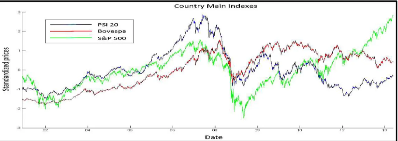
Figure 1 - Standardized Prices for the main equity index of each country
I find that portfolios that combine the different signs given by the trend following
strategies outperform the respective indexes in Sharpe ratio terms, significantly reducing
at the same time the drawdown levels. Furthermore, while for the Portuguese and
Brazilian market the small cap was the one that displayed better risk-adjusted returns, for
the US it was the large cap counterpart that performed better. Perhaps, the most important
result was the massive reduction of volatility and the maximum drawdown levels. From
a risk-averse investor perspective, the strategy succeed to present equity like returns with
bond like volatility and drawdowns (Faber, 2013), being a good alternative for investors
that look for long-term stable returns that do not compromise a large part of the
11 It is important to refer that these results should not be viewed as a finalized portfolio1, but
as an attempt to identify equity market properties across each country, to signal investors
of the best way to approach each specific market.
The remaining of the report is organized as follow: in section 2, I present the literature
review related with the topic studied; in section 3, I present the data and methodology
used along the work project; In section 4, I display the main results for each strategy
across the three markets; in Section 5, I present the Combining (Final) strategy for each
index; in section 6, it’s possible to find the strategy applied to a sub-sample period that
confirms the good performance exhibited before; for last, section 7 concludes the report
with the main results found.
2. Literature Review
Trend following and mean reverting strategies represent an important segment of
financial literature. There is a growing evidence that using this type of strategies for a
variety of asset classes exhibits better results from a risk-return perspective. As an
investment style, trend following has been used for a relative long time. Back in the
twenty century, Jesse Livermore, one of the icons of Wall Street, introduced this new
investing approach. He explicitly stated, “big money was not in the individual fluctuations
but in the main movements, that is, not in reading the tape but in sizing up the entire market and its trend” (Lefèvre, Edwin, 1923, p.54). Trend following relates to market
momentum: when prices move in one certain direction in one period, it is likely to
1 Along this work project, I focus completely in the equity market side, making no attempt to diversify at
12 continue on that direction in the next. Mean reverting will be the opposite: when the prices
move far away from a certain historical mean, a correction is expected to happen in the
next period, pushing those prices to more “reasonable” values.
Along the recent history, these type of strategies are getting more and more attention as
investors try to contradict the market efficiency theory and obtain alpha returns above the
market. In theory, abnormal returns or market anomalies are a chance result, an
overreaction/underreaction of stock prices to information that tends to disappear in the
long-term (Fama, 1997). According to the Efficient Markets Hypothesis (EMH), market
mirrors all the information available to market participants at any given time (Fama,
1970). In other words, it is believed that stocks always trade at their fair value and is
impossible to outperform the market through stock selection or market timing.
Nevertheless, there is extensive evidence that contradicts and reject the EHM, and clarify
how it is possible to predict future returns based on past returns (Jegadeesh and Titman,
1993). For instance, in the Portuguese market, the hypothesis of daily returns linearity is
rejected, leading to the possibility of excess profit opportunities in the market (Afonso
and Teixeira, 1998). Nevertheless, the introduction of the Euro as well the development
and increased integration of financial markets, helped to increase efficiency in the
Portuguese market. Similarly, institutional inefficiency seems to be present in Brazil. As
Medeiros refers, “the Brazilian market would be prone to be manipulated by informed
13
Market Hypothesis. Besides, smaller markets should be more susceptible to this sort of irrational behavior” (Medeiros, 2005, p. 10).
Liquidity, when put in a context of market inefficiency, plays an important role in returns
predictability. Indeed, prices are closer to a random walk benchmark during periods of
higher liquidity. Return predictability diminishes during liquid periods as increased
arbitrage activity during these periods enhances market efficiency (Chordia et al., 2007).
Trend following strategies succeed to improve adjusted returns and achieve non
risk-factor explainable returns independently of market’s characteristics. Furthermore, the use
of trend following strategies is not exclusive to a certain asset class. When compared to
equally weighted portfolios, trend following presents better risk-adjusted returns for
commodities, equities or even bonds (Clare et al., 2012). Additionally, the benefits are
not exclusively related with enhanced returns as shown by Clare et al.:
“[…] a pure trend following strategy, or one overlayed on a momentum strategy with volatility-adjusted weightings, reduces drawdown compared to buy and hold benchmark. We believe that such strategies would be ideal for risk averse investors [...]” (Clare et al., 2012, p.16).
Trend Following strategies act as signal filters, amplifying high frequency noise and
inducing short-term positive autocorrelations (Farmer et al., 2001). The features of this
type of strategies makes them suitable for any country stock market, being the results
dependent on a set of characteristics like size, value or liquidity. For instance, it has been
proved the existence of size effect across the stock market: small caps stocks tend to
14 likely to be present across trend following or momentum strategies as Jegadeesh and
Titman documented:
“In fact, if the profits are not factor related, the strategies are likely to generate higher returns when they are implemented within the small-firm subsample that consists of less actively traded stocks and to generate lower returns when they are implemented within the large- firm subsample”(Jegadeesh and Titman, 1993, p.76).
Therefore, the small cap universe tends to generate higher momentum, though one
possible explanation for these abnormal returns can be the impact of higher trading costs
on price behavior, giving the illusion of trading opportunities when they do not exist
(Lesmond et al., 2002). Despite the high transaction costs associated with illiquid assets,
liquidity trading can be profitable and contradict the market efficiency theory. In the
existent literature there is not a clearly and unanimous definition for liquidity or
illiquidity. Liquidity can be seen as the order flow impact in price that results from
adverse selections and inventory costs (Amihud, 2002). Strictly speaking, for the same
set of expected cash flows, more liquid assets are expected to have higher prices
(premium) while less liquid assets are expected to have lower prices (discount). Often
investors also use stock turnover as proxy for liquidity (Datar et al., 1998),
volume-to-earnings ratios (Chen et. Al., 2010) or even size, as small caps are believed to be more
volatile and less liquid than the large cap ones. Furthermore, liquidity also varies at
country level. Once we move from larger financial markets (e.g. US) to smaller ones, the
liquidity effect tends to be stronger and more significant as mentioned before.
Consequently, liquidity can also be an obstacle to investment. Institutional investors are
often concerned with the relative riskiness of emerging markets. More particularly, their
15 foreign investment (Chuhan, 1994). Nevertheless, as less liquid stocks tend to outperform
their more liquid counterparts across time, liquidity can be used as an investment style
(Amihud and Mendelson, 1986). Taking advantage of liquidity market premium, by
favoring less liquid stocks at the expense of more liquid ones turns out to be profitable,
obtaining alpha/beta excess returns (Chen et. Al., 2010).
At the end, trend following strategies are a better alternative to the traditional 60% stocks
and 40% bonds asset allocation. As Mohamed El-Erian, former manager of the Harvard
endowment, stated, “Diversification alone is no longer sufficient to temper risk. In the
past year, we saw virtually every asset class hammered. You need something more to manage risk well”2. As different markets and non-correlated asset classes experience large declines simultaneously, and the normal benefits of diversification disappear, trend
following can be a good solution. The strategy signals when an investor should exit a
risky asset class in favor of risk-free investments, leading to equity like returns with bond
like volatility and drawdowns (Faber, 2013).´
3. Data and Methodology
To explore the possible value in trend following approaches to equities, I considered three
broad markets: USA, Brazil and Portugal. The purpose of this work project is to study
strategy performance across different types of equity markets within each country,
namely the small cap market, the large cap market and the main stock index. Therefore,
the nine equity indexes used are: Brazil large cap index (Russell), Brazil small cap index
16 (Russell), Bovespa index, Portugal large cap index (MSCI), Portugal small cap index
(MSCI), PSI 20 index, Largest 100 stocks in market cap (S&P 100 index, USA), smallest
600 stocks in market cap (S&P 600 index, USA) and S&P 500 index. In addition to using
these financial indexes, other macroeconomic variables were also considered: Consumer
Price Index (USA, Portugal and Brazil), 3 month interest rate (USA), 6 month interest
rate (Portugal), Selic rate (Brazil) and volatility indexes (VIX and VOX, USA).
Regarding the interest rates, I used the ones with the shortest periodicity available, while
for Brazil I used the Selic rate that is often considered a proxy to the Brazilian short-term
interest rate. All the data used in this work project was collected and analyzed on a daily
basis. The data sample covers the period between January 2002 and December 2013 for
Brazil and US, while for Portugal it starts in January 20043 and it goes as well until
December 2013. I decided to use the method introduced by Faber (2006). Along the third
section, the methodology used repeats itself with small changes dependent on the variable
studied. The system is as follow (30-day moving average with volatility filter example):
If, P (t) > Mean (P (t : t-29)) + Standard Deviation (P (t : t-29));
Strategy Signal = 1
If, P (t) < Mean (P (t : t-29)) - Standard Deviation (P (t : t-29));
Strategy Signal = -1 Otherwise,
Strategy Signal = 0
Some important observations regarding the system:
1) P = daily price and t = day;
2) t ∈ [30 : end] , we lose the first 30 observations;
17 3) As referred along this report, some strategies will use the volatility filter while
others don’t (only use the mean moving average);
4) Given that, some variables have a contrarian effect in the indexes, the strategy
signals in that case will be the opposite.
In the fourth section, the signals given by the different strategies are combined in order
to reach the final output for each index.
The trend following filter will be a binary outcome in terms of equity allocation with
either 100% investment in the respective index (Long, 1) or selling 100% the index
(Short, -1). This variation4 to the method used by Faber (2006) and posteriorly by Clare
et al. (2012), has the objective of approximating the strategy to the actual market
conditions faced by investors. Additionally, transaction costs are also not considered.
4. Results
4.1 Long Only
I start by examining the main indexes behavior across the three countries and its
respective small and large cap counterparts from a buy and hold strategy perspective. The
Long only strategy descriptive statistics for the US (Panel A, B and C), Portuguese (Panel
D, E and F) and Brazilian (Panel G, H and I) related indexes, can be found in every table
presented along this report, identifiable by the ticker index.
18 Compound annual returns range from approximately -3% to 20% with the MSCI LC PT
and Russell SC BRL representing these extremes, respectively. The risk adjusted return
winner was precisely the index that represents Brazilian small cap stocks with a Sharpe
ratio5 of 0.92. Furthermore, in the overall picture, the Brazilian indexes exhibited the best
results from a risk adjusted return perspective. Across the three countries, we observe that
market behavior is coherent with actual literature that suggests the higher performance of
small caps over large caps in the long term, although usually at the expense of higher
volatility. The theory holds for the US and Portuguese market. However, in the Brazilian
one, the small cap index presented both higher returns and less volatility (19.82% and
21.61%, respectively) when compared with the country main index Ibovespa (10.89%
and 29.02%). Figure 2 demonstrates Bovespa’s dependence on the country’s biggest
stocks.
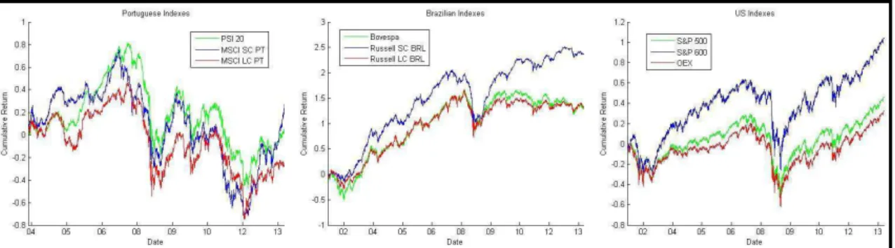
Figure 2 - Long Only strategy across the three markets
As one should expect, the three indexes revealed a homogeneous behavior. Nevertheless,
while Russell LC BRL index returns were very similar with the Bovespa ones, the Russell
SC BRL index clearly outperformed the latest in the sample period. In addition to the
improved return and volatility, the latter also grants a lower maximum drawdown
(approximately 34%) compared with the Bovespa one (approximately 54%).
5 The Sharpe ratio, introduced by William Sharpe in 1966, is a way to examine the performance of an
19
4.2 Trend Following
In this section, I analyze the impact of implementing pure trend following strategies to
the indexes mentioned before. I decided to use different moving averages (5, 30, 60, 90
and 250 days) in order to test strategy performance at a short, medium and long-term
level. Looking at the main indexes for each country (Table 1), the Portuguese one stands
out with enhanced annualized returns of approximately 1155% (using a moving average
of 60 days) while maintaining volatility levels constant. The index presented a Sharpe
ratio of 1.0851 while reducing the maximum drawdown by 50%. Furthermore, also
Portuguese large and small cap indexes presented trend following characteristics being
these ones stronger in the latter, where Sharpe ratios around 1 for 4 of the 5 signal lengths
were obtained. Indeed, one should expect these results for more volatile markets like the
Portuguese and Brazilian ones. Figure 1 (Section 1) illustrates the standardized prices for
the main index in each country. First, is easily observed that the PSI 20 index presented
a wilder behavior than the S&P 500 and Bovespa indexes, as it tended to “jump” more,
therefore being a better candidate to bet on directional moves. Second, the auto regression
levels can be used as proxy for the probability of having trend following or mean reverting
properties. The daily autocorrelation for the PSI 20 (0.0643) supports the strategy’s
performance success. The positive autocorrelation can be interpreted as the probability
that a positive return is followed by a positive return in the next day and vice-versa.
Additionally, the strategy maintained the Kurtosis value more or less constant, while for
the skewness, is possible to observe a shift from a negative skewned distribution to a
positive skewned one. A positive skewness implies that the mean of the sample is greater
than the median. In other words, it is more volatile than average when making money and
20 the maximum drawdown: the strategy was able to reduce extreme results in negative
terms while improving the positive ones. Despite presenting higher levels of volatility,
the MSCI LC PT did not perform so well when compared with its small cap counterpart.
The best Sharpe ratio (0.4249) was obtained using a moving average of 90 days, leading
me to conclude that, from a risk-adjusted return perspective, pure trend following
strategies are not the most suitable for the large cap market in Portugal. In the case of the
MSCI SC PT, the strategy obtained the best results across all indexes studied in this
section, as stated before. The mentioned index presented strong short and medium term
trend following properties being these ones maximized when using a moving average of
5 days (Sharpe ratio equal to 1.24). The index daily and monthly autocorrelations (0.0636
and 0.2 respectively) were similar to the PSI 20 index one, foreseeing good results from
a trend following perspective. The strategy managed to improve returns in approximately
1274% while reducing the maximum drawdown from 85% to 20%. I can conclude that
the success of trend following strategies in the Portuguese main index is mostly driven
by the small cap performance than its counterpart. These results are in accordance to the
findings of Soares and Serra (2005), which proved how the Portuguese stock market
shows momentum in the short/medium term, reverting to a certain mean after the 18th
month.
Thus far, I focused in the Portuguese case. The next step is to assess the behavior of the
strategy in the Brazilian market. The baseline strategy (Long only) clearly highlights
Bovespa’s greater returns (10.89%) when compared with PSI 20 and S&P 500. One
would expect that these high returns would come at the expense of higher volatility
values. In spite of that being true, the relation return/volatility is noticeably higher in the
21 trend following strategy, comparing once again with the baseline long only strategy. From
a Sharpe ratio perspective, the strategy showed higher performance when using a 30 and
60 days moving average, nevertheless the signaling strategy ended up adding low
incremental value to the index performance. The annualized return varied between
11.38% and -1.70% while the annualized volatility stayed constant around 29%.
Although, along the different signal lengths, the maximum drawdown increased to values
that one may already find prohibitive. The negative autocorrelation (-0.01) may suggest
mean reverting strategies as a better candidate to Bovespa index, nevertheless the value
seems to be considerably close to zero to take significant conclusions. The Russell LC
BRL presented more or less the same behavior as the Bovespa index, when tested for
trend following properties. Once again, the strategy failed to present enhanced
risk-adjusted returns, presenting on average lower Sharpe ratios than the long only strategy.
The opposite happens in the Russell SC BRL case. Similar to the Portuguese example,
the strategy seemed to perform extremely well, presenting Sharpe ratios between 1.09
and 1.42. If the returns of the small cap index were already impressive by themselves, the
strategy was able to improve them, attaining incremental returns of approximately 10%
(30 day moving average). The similarity between the two markets was once more
emphasized by its Kurtosis and skewness levels. The Kurtosis value of 8 proves that the
returns are far away from presenting normality properties since they present fat tails
(relative high number of extreme results). It is also possible to see again a shift from
negative skewed returns to positive skewed returns. Nevertheless, in this set of
performance statistics, the maximum drawdown did not perform so well as in the
Portuguese case. While in the long-term, the strategy presented lower maximum
22 the day moving average example. At the end, the trend following strategy (using a
30-day moving average) for the Russell Small Cap Brazil presented the best risk-adjusted
returns but at the same time, the highest peak in portfolio’s value lost.
Finally, the S&P 500 was the main index that presented the worst results. The returns
always dropped despite the signal length, leading to very low and even negative Sharpe
ratios. The poor performance of the strategy is highlighted by the maximum drawdown
values. The maximum drawdown was always above the total value of the portfolio,
making this strategy impossible to follow by any investor. Likewise, trend following
applied to the OEX index and the S&P 600 showed a similar behavior. Both indexes
failed to present enhanced returns in relation to the baselines portfolios, leading to,
non-investable Sharpe ratios. Being the most efficient market among the three, this type of
inefficiencies tend to disappear and be corrected faster. Furthermore, the negative daily
autocorrelations lead me to believe in the success of contrarian strategies in this market
instead of pure trend following strategies.
Figure 3 - Pure Trend Following strategies across the three markets
So far, I can take some conclusions regarding the pure trend following strategies.The
three examples studied in this section, have shown that pure trend following is a
risk-lover like strategy. All the benefits come from the returns side, whereas volatility stayed
constant across the different signal lengths used. Furthermore, the Portuguese and
23 following context, however only the PSI 20 was able to similarly replicate the results
performed by its small cap constituent. There is a particular literature that documents the
influence of large caps in the Bovespa index and how they tend to shape the index
behavior, however I will have the opportunity to study this hypothesis further ahead in
this work project.
4.3 Mean Reversion
Having shown the performance of trend following strategies across the three different
markets, the next logical step is to study mean reverting properties across the referred
markets. Given the strong results obtained in the last section, it is expectable a poor
performance of the PSI 20 index when given a mean reversion signal. Table 2 presents
the Mean Reversion strategy descriptive statistics for the three main indexes and its
respective small and large cap indexes.
For the Portuguese case, the strategy failed to present positive returns independently of
the signal length given. This scenario complements the results obtained in the last section:
the Portuguese market presents strong trend following characteristics in the short/medium
term.
Regarding the Brazilian market, Chaudhuri and Wu (2004) documented the evidence of
mean reversion in stock prices using emerging markets. Their results suggested the
existence of mean reversion for several emerging countries as Brazil (1% significance),
nevertheless, the speed of reversion supported (30 months) goes beyond the time lengths
studied in this project. My results for the Brazilian market end up being similar to the
ones found in the Portuguese market. Again, the strategy failed to present better
24 repeated itself. I can conclude that Bovespa and the Brazilian Large cap market exhibited
the most unpredictable returns across the three markets as both initial strategies failed to
improve significantly the long only strategy Sharpe ratios. Given the characteristic high
returns of this market, strategies that explore the volatility side instead of the returns one,
may offer better value-added performance.
Contrarily, the US market displayed some interesting results, mainly in the short-term
horizon. For the S&P 500 example, it was possible to increase returns by 198%, using a
5-day moving average, reducing at the same time the volatility values. At a 30/60-day
basis was also possible to observe some mean reversion, nevertheless it was using the
5-day signal length that the best Sharpe ratio was obtained (0.8361). As mentioned before,
the daily returns negative autocorrelation (-0.10) already forecasted this scenario. Besides
offering better risk-adjusted returns, the strategy also reduced the maximum drawdown
from 64% to 14%. This is one of the most important indicators for investors as, frequently,
the liability of undertaking this type of strategies is the capacity to hold it in times of
market distress. Once again, the strategy’s extreme results, represented by the high
kurtosis value (32.2), confirm the expected returns’ non-normality6.
Figure 4 - Pure Mean Reverting strategies across the three markets
When applied to the OEX index (Large cap) the strategy performed even better, attaining
a Sharpe ratio above one (using 5-day moving average). In this case, the high kurtosis
25 was followed by a relatively high positive skewnsess, leading me to conclude that the
strategy was more constant when losing money than making it. For the S&P 600 (Small
cap), the results were identical but at a lower degree: poor performance in the
medium/long-term while in the short-term the salient result was the volatility reduction.
4.4 Calendar Market Anomalies
There is a vast literature that tests and documents different types of market anomalies that
tend to contradict the efficient market hypothesis. In this section, I will analyze three
specific ones: the Monday effect, the January effect and the turn-of-the-month effect. The
goal is to verify how the strategy that explores each calendar anomaly performs when we
move from the most liquid market (US) to less liquid markets (Portugal). The weekend/
Monday effect refers to the phenomenon in financial markets in which Monday returns
tend to be lower compared with the previous Friday ones. There are multiple explanations
for this market singularity as French (1980) and Richard Thaler (1987) acknowledged.
This effect has been linked to high volatility in the weekends as well simply faded
optimism by traders during this period. Across the three strategies, this was the one that
presented less optimistic results. Nevertheless, it managed to exhibit positive sharpe ratios
in 8 of the 9 indexes studied. The strategy descriptive statistics can be found in Table 3.
The sharpe ratios obtained for the US market when tested against the weekend effect
ranged between 0.13 and 0.19. I will highlight the S&P 500 since is the index that
exhibited the best results. The Kurtosis value clearly stands out when compared with the
long only strategy value for the S&P 500. It is important to remember that, the
26 leading to a distribution with larger fat tails. Despite showing extreme results across the
sample period, the maximum drawdown was only 20%, what represents a clearly
improvement to the baseline portfolio. When applied to the Portuguese market, strategy’s
behavior was quite similar, though it should be noted the negative result displayed by the
small cap index. Once again, the maximum drawdown values were reduced across the
three indexes being in accordance with the high Kurtosis value: by considerably reducing
the investment /trading days, we reduce our exposure to the market and the value at risk
that comes with it. For last, the Brazilian market also displayed this type of anomaly,
nevertheless at higher significance, having its peak in the small cap index (Sharpe ratio
of 0.39). The next market anomaly studied was the January effect. The January effect
refers to the buying rally during the first week of January, following the drop in price
revealed in December. As Thaler (1987) and Gu (2002) documented, this pattern can be
explained by year-end tax losses selling of stocks to offset capital gains and how investors
tend to buy them back in January with the help of year-end bonuses. Notwithstanding,
this phenomenon has been less noticeable in recent years, even for the small caps, as
markets have adjusted to it across time. My results end up being contradictory, as both
smallest and biggest Sharpe ratios were achieved by two different small cap indexes.
Regarding the US market, it showed better performance when applied to S&P 500 and
the large cap market, exhibiting enhanced Sharpe ratios of 0.57 and 0.48, respectively. I
will focus on a return/volatility analysis, since it is useless to examine Kurtosis and
Skewness when I am only trading January’s first week each year. Similarly, PSI 20 and
MSCI LC PT indexes were the winners for the Portuguese market, as the small cap index
failed to present positive returns opposing common literature but in accordance with the
27 displayed a constant behavior exhibiting enhanced risk adjusted returns for the three
indexes. Contrarily to the examples shown before, the small cap index was the one with
the best sharpe ratio (0.63) nevertheless still below the baseline index one. I decided to
leave the turn-of-the month strategy to the end since it was the one with the best and most
constant results across the three markets. The turn-of-the-month phenomenon refers to
the positive pattern found in returns at the end of each month: stock prices rise during the
last days and the first days of each month. Kunkel et al. (2003) document the persistence
of this effect in several markets, while Nikkinen et al. (2006) acknowledged how the
effect of macroeconomic news announcements at the end of each month help to explain
this market anomaly. In this sample period, the effect was not only presented in the three
markets, as also, surprisingly, exhibited better Sharpe ratios in relation to the baseline
benchmark in each single index studied. Nonetheless, the best were evidenced by the
Brazilian market with astonishing Sharpe ratios ranging between 1.14 and 1.59. It is
important to mention how, contrarily to the US and Brazilian market, the Portuguese
Large cap index performed relatively better than the small cap one (Sharpe ratios of 0.69
and 0.41 respectively). Furthermore, the maximum drawdowns were comparably lower
than the baseline index ones, being in accordance with the success of the strategy.
Figure 5 - Calendar Anomalies (all together) strategies across the three markets
Across the three strategies studied in this section, is possible to distinguish some relatively
high/low skewness values. Nevertheless there is not an evidently correlation between
28 clear picture over investor Skewness preference. Exclusively in this section, I agree with
the theory presented by Scott and Horvath (1980). Positively skewed returns will be
preferred as they offer a limit downside while boosting at the same time the potential
upside. By other words, the lottery effect will kick in the event of the appearance of
market anomalies, leading investors to overweight the fat tail until the crowding out effect
eliminates the inefficiency from the market. Despite the vast literature, it is possible to
conclude that these market anomalies persist independently of the market characteristics.
4.5 Consumer Price Index (CPI)
Up to this point, I have considered pure strategy performance within each index and which
are the advantages that one may take from it. Hereafter, I will concentrate on
macroeconomic variable correlation with stock returns, and how its behavior can or not
assist to predict the direction of the stock market. In this section, I will study how the CPI
can help to shape equity returns. The CPI influence on US stock returns has been well
established in the economic literature by, amongst others, Sharpe (2002) and Sirucek
(2012). Sharpe (2002) documented how changes in expected inflation affected long-run
return on stocks, while Sirucek (2012) examined the negative impact of inflation on share
prices. Here I examine the indexes response to CPI from a trend following perspective
with a volatility filter. The volatility filter will guarantee that I only go long or short if the
macroeconomic variable exceeds a certain acceptable range. As CPI is a contradictory
indicator, I go long when its values are below the moving average mean minus one
29 In the S&P 500 example, the strategy performed quite well, exhibiting improved Sharpe
ratios in three of the four signal lengths studied. As one can notice in Table 4, there are
no values for the 5-day moving average since it does not seem logical to test a monthly
indicator against such short period7. The best scenario (S&P 500) was obtained when
using the largest signal length possible, improving returns by 188% while maintaining
volatility more or less constant. In addition to reveal better risk adjusted returns, the
strategy also improved maximum drawdown and returns symmetry. The Kurtosis value,
despite being high, was in accordance with the one exhibited by S&P 500. Therefore,
these results were in agreement with actual literature, and given that the CPI is a lagging
indicator it is reasonable to have the best results using the highest signal length. For the
US large and small cap market the strategy behavior was similar, nevertheless the OEX
index presented the best improvement in returns when compared with the long only
strategy. Using a signal length of 250 days was possible to obtain a Sharpe ratio of
approximately 0.52, 3.7 times higher than the long only one.
For the Portuguese scenario, the Consumer Price Index also helps improving index
results. The benefit came once again at a long-term horizon (90 and 250 days length),
where the PSI 20 displayed Sharpe ratios of 0.443 and 0.8341. Similarly to what was
concluded in the previous section, the strategy does not improve volatility levels,
nevertheless the enhanced returns are reasonably significant. Contrarily to the US
scenario, the maximum drawdown increased from 64.3% to 75.7% (superior returns came
at the expense of a higher value at risk). Furthermore, the strategy turn out being effective
also for the Portuguese large and small cap market, although, in contrast to the US
7 CPI values are only revealed at the end of each month and a 5-day moving average would lead to
30 example, the best results were evidenced by MSCI SC PT index. Regardless of the
upgraded Sharpe ratio for the MSCI LC PT index (0.3669), it was the small cap index,
that using a 250-day signal length, presented the best Sharpe ratio (0.9086). In accordance
with PSI 20 index, the strategy achieved better returns. Even so, it failed to reduce the
maximum drawdown. Notwithstanding the high maximum drawdown value (83%), it is
important to refer that, by allowing short selling, I assume the possibility of taking
advantage of severe declines in the market leading to results that are more volatile than if
I wouldn’t. Actual literature related with the subject failed to find statistical significance
on the influence of Portuguese inflation in the national stock market.
For last, inflation in Brazil is one phenomenon that has been widely study given its
irregular behavior. Inflation has been an “old enemy” of Brazilian economy for quite long,
presenting several periods of hyperinflation across its history. Despite showing signs of
improvement in the last years, inflation is still considerably high when compared with,
per example, the US CPI values8. Therefore, as high inflation tends to create uncertainty
and distrust in the market, I will observe how that traduces in strategy performance. When
applied to Bovespa, the strategy exhibited improved performance using the three largest
signal lengths, nevertheless the best risk-adjusted returns were obtained using a moving
average of 90 days (Sharpe ratio of 0.5707). The strategy enhanced returns by 51% in
relation to the baseline index, although those returns come at the expense of a higher
maximum drawdown (60.35%). Despite the relatively high kurtosis and maximum
drawdown values, they were in accordance with the ones presented by the index. The
large and small cap markets response to the strategy was similar to the main index one,
31 yet the Russell SC BRL exhibited once again the best Sharpe ratio across all the indexes
studied (1.267 , 250 day moving average).
Figure 6 - CPI strategies across the three markets
Alike the pure trend following example, using the Consumer price index, the strategy was
able to improve the already high returns of the Brazilian small cap index from 19.820%
to 27% maintaining volatility constant at approximately 21%. Nevertheless, it is
important to refer the move from negatively skewed returns to positively skewed returns
and the considerably high increase in the maximum drawdown. Eid (2005) documented
how the Bovespa index turned out being less efficient after the Plano Real9 and the
stabilization of inflation, leading to a shift of excess returns in the stock from a normal
distribution to a less well-behaved one.
4.6 Interest Rates
The second macroeconomic variable to test is the short-term interest rates. As mentioned
in the data section, I will use the Brazil target rate SELIC as proxy for the Brazilian
short-term interest rate, the 6-month government bond yield for Portugal and the 3-month
government bond yield for US. Similarly, to CPI, interest rates are a contrarian and
9 The Plano Real (1994) was a set of measures taken to stabilize the Brazilian economy and mitigate
32 lagging indicator: as external funding becomes more expensive, stock prices are expected
to go down and vice-versa.
Sirucek (2012) documented this phenomenon proving the negative impact of US interest
rates on Dow Jones index. However, when tested to S&P 500, the impact was positive,
contradicting economic theory. In this case, the strategy exhibited a higher performance
for the S&P 500 and the OEX than to the S&P 600, succeeding to achieve positive returns
across four of the five signal lengths. Contrarily to the Selic rate, the 3-month bond is
quoted in a daily basis, leading to better results in the medium-term than in the long term
(250 moving average) as shown in table 5. The best result for the S&P 500 was obtained
using a 30-day signal length leading to a Sharpe ratio of 0.6678, 3.56 times higher than
the baseline index one. Once again, is important to refer the use of a volatility filter in
order to obtain stronger results, anticipating a lower exposure to the stock market. The
percentage of positive days and the maximum drawdown results confirm this idea. Given
that the daily interest rate values were often between the out-of-the-market10 stipulated
ranges, the strategy end up presenting a relatively low percentage of positive days
(25.92%), although it also reduced the maximum drawdown from 64% to approximately
29%. Additionally, the volatility filter also affects the distribution of returns. The frequent
neutrality against the market leads to several observations where the strategy’s daily
return is zero. Therefore, every time that I decide to go long or short, the returns (positive
10 Out-of-the market range refers to the values between the moving average mean plus one standard
33 or negative) will always be interpreted as extreme results, as the mean of the distribution
will be close to zero.
Figure 7 - Interest rate strategies across the three markets
For the OEX example, the strategy also exhibited better results when using a 5 and
30-day signal length, while for the small cap index, conditioned by the baseline index high
Sharpe ratio, the strategy failed to present enhanced risk adjusted returns despite the
signal length used.
The Portuguese and Brazilian markets were the ones where the strategy of using interest
rates to predict market’s direction performed better. I will now focus on the large and
small cap indexes, as they were the ones with the most significant results. Looking at
panel E (table 5) it is easy to identify two opposite results: while in the MSCI LC PT
index the best Sharpe ratio was obtained using the lowest signal length, in its counterpart
the best Sharpe ratio was obtained using the highest one. Despite the overall enhanced
Sharpe ratios, the one for the large cap market is quite suspicious (0.7968). From a return
perspective, it is possible to observe how the return of 14.94% is completely misaligned
with the ones obtained using other signal lengths, leading consequently to relatively lower
Sharpe ratios. One possible explanation could be the ineffectiveness of the 5-day moving
average to avoid market noise11. As these results are smoother for the PSI 20 and MSCI
34 small cap Portugal index and interest rates tend to lag, I will focus this analysis in the
higher signal length examples. Hereupon, the clear winner was the small cap index, where
the strategy succeeded to increase annualized return from 2.340% to approximately 15%
reducing at the same time the index volatility. Furthermore, using the highest signal
length, was possible to approximate the Kurtosis value to the one presented by the
baseline index, while exhibiting a clearly improved maximum drawdown. It is important
to refer that, despite the relative inferior strategy performance for the PSI 20 and MSCI
Large Cap Portugal index, the results showed better risk-adjusted returns than the
baselines index ones.
For last, the Brazilian market exhibited Sharpe ratios that clearly outperformed the other
two markets. As mentioned in the data section, the Selic rate is a monthly indicator,
therefore it does not seem logical to test it for a moving average of 5 days. Panel G, H
and I show how the strategy presented superior risk adjusted returns for the three indexes,
often at the expense of a higher maximum drawdown. Once again, I will focus my
attention in the small cap market, where were obtained Sharpe ratios above one for three
of the four signal lengths tested. Despite the surprisingly high Sharpe ratios, these results
are in accordance with actual literature on the subject. For instance, Hersen et al. (2013)
documented this negative relationship, proving how a 1% increase in Selic rate leads to a
1,000 points drop in the Bovespa index. The strategy ended up being more “active” for
the small cap index as the positive days percentage demonstrates, while return’s
distribution fat tails got smoother with increases in the signal length. It is important to
mention, how the extremely good performance of the Brazilian indexes across the sample
period influenced the results, nevertheless the strategy managed to turn them even more
35
4.7. S&P 500 spillover effect and Volatility index
Thus far, I studied the benefits of using macroeconomic variables to predict market
direction. In this section, I will study the possible spillover effect of the US market in the
Brazilian and Portuguese market, while for the US market I will study the behavior of the
trend strategy when tested against volatility indexes. If in the first example is obvious
why I only test two markets, in the second, the reason is the lack of available data
(volatility indexes) for the Portuguese and Brazilian markets. Therefore, in order to avoid
misleading results by using benchmark indexes, I decided to exclude both countries from
the volatility index analysis.
It is logical to believe in the spillover effect of S&P 500 over different stock markets
across the world: being one of the most followed indexes, its performance can shape
investor sentiment, leading to a wave of optimism or pessimism across the other countries
stock markets.
In the Portuguese and Brazilian markets, this idea ended up being true, nevertheless with
more incidence in the Portuguese one. Table 6 confirms how the strategy exhibited
improved Sharpe ratios despite the signal length used for the PSI 20 index. Indeed, when
the S&P 500 is trading above its 90 days mean, it seems a good scenario to go long on
the Portuguese main index and vice-versa. Furthermore, this strategy presented the best
risk adjusted returns for the PSI 20 (Sharpe ratio of 0.8873), while exhibiting at the same
time a relatively good performance for the large and small cap indexes. Despite the
enhanced Sharpe ratios for the large cap index, the MSCI SC PT index showed once again
the best performance, since was able to increase strategy returns by approximately 462%
36 values were also more in accordance to the baseline index ones and there was a clearly
negative skewness pattern over the three indexes.
The scenario repeated itself in the Brazilian market. Aside the benefits from a volatility
perspective for the Bovespa and the Russell LC BRL indexes, the strategy exhibited also
significantly enhanced returns in the medium/long term for the small cap index. The
maximum drawdown was more or less constant across all signal lengths, but conditioned
by the relative low value exhibited by the baseline index (34%). The Kurtosis value
increase was quite significant leading to more extreme results than usual, being the
negative returns the mainly foundation of this fatter tails (negative skewness). Actual
literature on the subject confirms this tendency. Passos et al. (2014) documented the
influence of several US stock indexes over the Brazilian stock market, findings that help
to back up the theory of increasingly and interdependent financial markets.
The last variables to be analyzed are the volatility indexes, more precisely VIX (S&P 500
and S&P 600) and VXO (S&P 100). Regardless of VIX being the index directly related
to the S&P 500, I will use it as a proxy for the S&P 600 since the only small cap volatility
index for the US market is not available for the entire period covered in this work project.
Chung et al. (2011) makes the case for the predictive informational content presented in
VIX and S&P 500 index options, being its effectiveness higher when the market is over
an extreme/volatile period. The strategy exhibited strong results for the S&P 500 and
OEX indexes, while for the S&P 600, clearly conditioned by the assumption mentioned
before, the strategy only exhibited enhanced Sharpe ratios in the very short-term.
Similarly to the strategies before, the volatility filter used led to a low percentage of
positive days, as the number of days out-of-the market were quite substantial (Table 6).
37 transaction costs borne by the investor. Often referred as the fear index, is important to
clarify that VIX represents the market volatility expectations for the next 30 days.
Figure 8 - S&P 500 spillover effect and VIX/VXO strategies across the three markets
Therefore, it is logical to assume that the strategy will perform better in the short term, as
the index tends to get out of context as signal length increases. For both S&P 500 and
S&P 100 indexes, the strategy presented the best Sharpe ratios using a signal length of 5
days (0.6514 and 0.8377, respectively). It is possible to observe how the index predictive
effect tends to disappear as it moves to higher signal lengths, influenced mainly by
decreasing annualized returns. Another identifiable pattern across the two indexes is the
maximum drawdown and skeweness values. The strategy aligned the best risk adjusted
returns with the lowest maximum drawdown values, while the skewness tends to shift
from high positive values (lower signal length) to negative values (higher signal length).
From the interpretation of the relatively high skewness values, I can conclude that the
strategy was reasonably stable when “making money” presenting occasionally some
extreme negative returns. The reductions in the maximum drawdown were substantial,
having its peak in the OEX example, where using a 5-day moving average was possible
to cut the maximum drawdown value in approximately 80%.
To conclude, VIX and VXO successively reflected investor sentiment, determining
consequently market direction on a short/medium term basis. Historically, the
38 many market cycles, nevertheless this relation seems to be more noteworthy during bull
and bear cycles (exhibits its higher peak and lower trough during these periods).
5. Combining Strategies
Having shown that applying trend following rules to equities can improve the risk return
characteristics of a certain portfolio, the next logical step is to create a final strategy that
combines the signals given by the different sub strategies studied. The objective is to find
better predictive signals and consequently improved risk adjusted returns. If for one
certain day, two different strategies present the same signal, I interpret it as strong
indicator to overweight/underweight the final strategy that specific day. Oppositely, if the
two signals are contradictory (e.g. long and short), I stay out of the market. In order, to
smooth over-fitting12 biased returns, instead of using all the strategies signs for each
index, I consider only the top 4/5 winners. Furthermore, the following section presents
the sub-sample13 analysis that re-confirms the good performance of the combining
strategy for a shorter period.
Table 714 displays the descriptive statistics for the combining strategy performance across
the nine indexes studied. Firstly, I recognize how the strategy managed to present Sharpe
ratios above one for all the indexes except the MSCI LC PT. Notwithstanding, should be
recalled that the Portuguese large cap index performance, from a long only perspective,
12 Over-fitting occurs when a strategy or a function is too closely fit to a limited set of data. Attempting
to make the model conform too closely to slightly inaccurate data can reduce its predictive power.
13 The sub-sample analysis refers to the same combining strategy but tested over the period between
Jan 2010 and Dec 2013.
39 was not only the worst among all indexes, as also exhibited a negative Sharpe ratio.
Therefore, despite the non-convincing absolute output, in relative terms the benefits are
substantial. From the return/volatility analysis, is possible to take some important
conclusions. First, the volatility behavior is clearly more consistent across the three
markets, with values varying between 6.3% and 10.78%, while the returns ranged
between 8% and 18.76%. Taking into account that for the long only strategy the volatility
values were all above 20%, the combining strategy succeed to present smoother returns.
Second, the source of better Sharpe ratios was not exclusively the volatility or the returns,
but a combination of both. Comparing with the long only strategy performance, is
possible to find a pattern where the benefits for the indexes that had relatively high
annualized returns (e.g. Russell LC BRL) came from the volatility side, while for the ones
that had relatively low returns (e.g. MSCI LC PT), came from both sides. Indeed, the
strategy for the Russell SC BRL index, that exhibited by far the best Sharpe ratio (2.10),
failed to improve the returns of its long only counterpart. Nevertheless, it reduced the
volatility levels in approximately 50%.
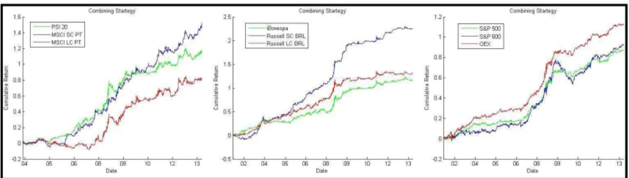
Figure 9 - Final (Combining) strategy across the three markets
The maximum drawdown, an indicator that gains further importance in long-term
strategies15, was also significantly lower with values ranging between 5.57% and 13.94%.
From a risk-averse perspective, the strategy brings huge benefits to investors when
15 Most of the times, investors have difficulties to stick to a certain strategy if drawdown values are
40 compared with relatively high drawdown values presented by the long only strategy.
These results are a consequence of the good strategy performance across distress periods
like the 2008 sub-prime crisis. For last, despite the high kurtosis exhibited by the final
strategy, the values are in accordance with the long only strategy ones, since they are
clearly conditioned by the January and end-of-the month strategies.
6. Sub-Sample test for the Combining Strategies
In this report, I choose to focus in investment strategies that, using long and short signs,
indicate where an investor should move in the market. I will now examine the
performance of the Combining (final) strategy for the period between January 2010 and
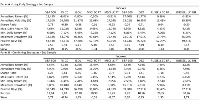
December 2013. Table 8 displays the performance and respective descriptive statistics for
the Combining strategy as well the long only strategy applied to the period mentioned
before. The universe of indexes and macro variables is the same, as well the methodology
used. The goal is to test how the strategy performed within a shorter period and
S&P 500 PSI 20 iBOV MSCI SC PT MSCI LC PT S&P 600 OEX RUSSELL SC BRL RUSSELL LC BRL
Annualized Return (%) 12,42% -8,01% -7,80% -0,30% -5,91% 17,40% 11,77% 9,86% -3,82%
Annualized Volatility (%) 17,10% 26,70% 21,87% 29,08% 27,04% 23,02% 16,55% 15,41% 18,89%
Sharpe Ratio 0,73 -0,30 -0,36 -0,01 -0,22 0,76 0,71 0,64 -0,20
Max. Daily Return (%) 4,63% 11,02% 4,98% 9,65% 11,75% 6,50% 4,32% 4,23% 4,42%
Min. Daily Return (%) -6,90% -7,12% -8,43% -9,25% -7,12% -8,86% -6,44% -7,06% -8,21%
Maximum Drawdown (%) 18,18% 84,07% 46,36% 99,61% 75,42% 23,91% 17,01% 19,73% 35,09%
Positive Days (%) 54,54% 51,61% 47,80% 52,16% 50,19% 53,73% 55,72% 52,23% 49,81%
Kurtosis 7,52 5,91 5,11 5,48 6,53 6,65 7,19 8,40 6,12
Skew -0,49 -0,15 -0,27 -0,34 0,02 -0,26 -0,46 -0,61 -0,41
Panel A - Long Only Strategy - Sub Sample
Indexes
S&P 500 PSI 20 iBOV MSCI SC PT MSCI LC PT S&P 600 OEX RUSSELL SC BRL RUSSELL LC BRL
Annualized Return (%) 5,54% 8,14% 3,96% 16,44% 8,88% 6,52% 7,14% 7,49% 3,62%
Annualized Volatility (%) 4,90% 9,99% 7,20% 11,27% 11,64% 6,90% 5,07% 6,36% 7,89%
Sharpe Ratio 1,23 0,81 0,55 1,46 0,76 0,94 1,41 1,18 0,46
Max. Daily Return (%) 1,87% 3,02% 5,06% 3,45% 4,11% 2,78% 2,13% 4,23% 6,15%
Min. Daily Return (%) -1,66% -4,41% -2,41% -4,83% -7,05% -2,59% -1,82% -2,54% -2,61%
Maximum Drawdown (%) 5,06% 10,48% 8,14% 7,24% 9,34% 15,51% 5,61% 5,96% 8,11%
Positive Days (%) 38,54% 44,59% 36,29% 36,87% 44,37% 39,80% 37,91% 39,43% 37,21%
Kurtosis 11,84 8,82 22,10 10,99 15,28 9,70 10,56 26,27 30,26
Skew 0,77 -0,34 1,45 -0,51 -0,57 0,60 0,85 1,35 1,79
Panel B - Combining Strategies - Sub Sample
Indexes
41 acknowledge the results without the influence of the 2008 sub-prime crisis, that due to its
particular effect in the stock market tends to influence positively the results of the
strategy.
Despite the Sharpe ratios of the combining strategy being relatively lower than the ones
exhibited previously, it is important to refer that the behavior of the indexes for this period
was also poorer, as the several negative annualized returns illustrate. The Portuguese
market performance was clearly influenced by the country crisis which started in 2010,
while for the Brazilian market the small caps continued its rally in opposition to the main
and large indexes that displayed negative Sharpe ratios. The MSCI SC PT was the clear
winner during this period moving from negative results to the highest one recorded among
all indexes, plus a significant 92,73% reduction in the maximum drawdown level.
More important is to observe that the properties of the combining strategy mentioned in
the previous section hold: enhanced risk adjusted returns for all strategies as well
significantly drops in the drawdown levels. Once again, is possible to observe how this
easy to implement strategy appeals for risk averse investors given the relatively low
volatility levels.
7. Conclusion
I have studied the performance of signaling strategies across different equity indexes. I
observed how trend following and mean reversion based in past prices improved
significantly risk adjusted returns when compared with the index by itself. Furthermore,
macroeconomic fluctuations also showed equity predictive properties along the three
42 interest rates similarly managed to present better Sharpe ratios in relation to the long only
strategy, nevertheless these results were constrained by the fact that some data
periodicity16was not matched. I would suggest testing the latter strategy using equity
indexes on a monthly basis for even more improved and significant results.
Calendar market anomalies seem to persist despite the vast literature around them, having
its peak in the end-of-the month/turn-of-the-month strategy. Despite the existence of valid
explanations, this type of pattern in the market confirms the difficulty in achieving and
maintaining the market efficiency hypothesis documented by Fama (1970).
The volatility indexes confirmed the strong predictive property of index options over
index future behavior, while the spillover effect of S&P 500 over other countries markets
was confirmed for Portugal and Brazil, with clear emphasis in the small cap market.
Besides the improvement in Sharpe ratio terms was possible to identify other type of
patterns. The Bovespa index (Brazilian reference index) seems to be driven by its large
cap components, confirming “it’s perverse” stock weighting as Oliver Leyland (Mirae
Asset Global Investments, 2013) quoted. Bovespa heavily weights stocks according to
liquidity and market capitalization17 leading to an increasingly two-tiered approach to the
Brazilian market by investors. At the end, the combining strategy behavior for the Russell
LC BRL and Bovespa index was very similar, while for other strategies like the CPI or
the S&P 500 the returns were incredibly high-correlated (See figure 6 and 8). This leads
me to conclude that the small cap market is clearly more attractive to investors than its
larger counterpart is.
16 CPI and interest rates (Brazil) have a monthly periodicity while the rest of the data is on a daily basis. 17 As of 2013, OGX (market cap of R$4.9B) had a weighting of 5.06%, while Ambev (market cap of