Ocean Sci., 11, 695–698, 2015 www.ocean-sci.net/11/695/2015/ doi:10.5194/os-11-695-2015
© Author(s) 2015. CC Attribution 3.0 License.
Technical Note: Remote sensing of sea surface salinity using the
propagation of low-frequency navigation signals
I. Astin and Y. Feng
Department of Electronic and Electrical Engineering, University of Bath, Bath, UK
Correspondence to:Y. Feng ([email protected])
Received: 11 September 2014 – Published in Ocean Sci. Discuss.: 19 December 2014 Revised: 4 August 2015 – Accepted: 17 August 2015 – Published: 7 September 2015
Abstract. This paper introduces a potential method for the remote sensing of sea surface salinity (SSS) using the mea-sured propagation delay of low-frequency Loran-C signals transmitted over an all-seawater path between the Sylt station in Germany and an integrated Loran-C/GPS receiver located in Harwich, UK. The overall delay variations in Loran-C sur-face waves along the path may be explained by changes in sea surface properties (especially the temperature and salinity), as well as atmospheric properties that determine the refrac-tive index of the atmosphere. After removing the atmospheric and sea surface temperature (SST) effects from the measured delay, the residual delay revealed a temporal variation similar to that of SSS data obtained by the European Space Agency’s Soil Moisture and Ocean Salinity (SMOS) satellite.
1 Introduction
Sea surface salinity (SSS) plays a fundamental role in the density-driven global ocean circulation and the water cycle. The latest remote-sensing SSS sources include the European Space Agency’s Soil Moisture and Ocean Salinity (SMOS) satellite (Reul et al., 2013) and the NASA Aquarius satellite (Lagerloef et al., 2013). This study attempts to explore a dif-ferent approach, by measuring the propagation delay of low-frequency ground waves transmitted over a path that consists entirely of seawater. For an all-seawater path, we expect sea surface salinity (SSS) to have a predominant effect on the delay variations.
The 100 kHz Loran-C transmitters in western Europe, pri-marily used for marine navigation in European and Arctic waters, have a long history of development. At the frequency used by these transmitters, the propagation of radio signals
occurs in two ways. The surface-wave component follows the curvature of the Earth, while the sky-wave component propagates through multiple reflections between the ground and the ionosphere. As Loran is a pulsed system, the dif-ference in path lengths between the ground and sky waves generally ensures that only the ground wave is tracked by the receiver, provided it is less than 2000 km from a transmit-ter (Pelgrum, 2006). However, under certain conditions a re-ceiver may track a combined signal (ground- and sky-wave) as close as 800 km, and this can contribute to errors.
The propagation velocity of the Loran-C surface wave is influenced by the refractive index of the atmosphere,η, and the electrical conductivity of the Earth’s surface. The atmo-spheric contribution to the time-of-flight (TOF) of the Loran signal, known as the primary factor (PF), is determined from this refractive index. The amount of time by which the TOF is increased by traversing over seawater instead of the atmo-sphere is called the secondary factor (SF).
However, the PF and SF values are usually computed within a Loran receiver under the assumption that η and the conductivity of seawater are both constant (e.g. Lo et al., 2009; Johler, 1957) and so depend only on distance. Their sum will be different to the actual TOF by an amount usually termed the additional secondary factor (ASF), i.e. ASF =TOF−PF−SF, which is generally assumed due to changes in conductivity (Lo et al., 2009). To help reduce this difference, fixed nominal ASF correction values, based on surveys, are also included within receivers. This receiver processing, however, assumes that there is no time variation in PF, SF or ASF, which is not the case, but is usually suf-ficient for many navigation purposes. In reality, the time-of-flight TOF is made up of both standard (or static) and time-varying PF, SF and ASF values (i.e. TOF=PF
696 I. Astin and Y. Feng: Remote sensing of sea surface salinity
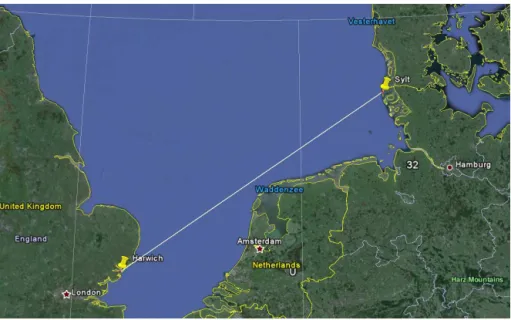
Figure 1.Loran-C propagation path between Sylt and Harwich (image from Google™Earth).
dard η)+PF (time-varying)+SF (standard)+SF (time-varying)+ASF (nominal, static)+ASF (time-varying)). By using the Global Positioning System (GPS) time and a (ru-bidium) atomic clock as a reference, it is possible to mea-sure the actual TOF to provide the time-varying (Loran) com-ponent (PF (time-varying)+SF (time-varying)+ASF (time-varying)) over an all-seawater path, which then may be at-tributed to atmospheric and sea surface properties. In real-ity, the receiver records the time-of-arrival (TOA) of Lo-ran ground-wave pulses, which is the sum of the time-of-transmission (TOT) for each transmitter (as measured by the station) plus the TOF, and receiver and station clock bias (i.e. TOF=TOA−TOT+bias).
2 Analysis and results
The time variations in ASF for the path (as displayed in Fig. 1) between the Sylt Loran-C station in Germany and Harwich, UK, were recorded by a fixed Reelektronika LO-RADD Differential eLoran reference station, operated by the General Lighthouse Authorities of the UK and Ireland (GLAs). This receiver calculates the variation in ASF by tak-ing the difference between the measured TOA and expected TOA (using expected TOF and using distance to calculate PF, SF, nominal ASF and TOE). The temporal resolution of these data is 30 s, and they were measured from February 2010 to July 2011.
For this reference station, Safar et al. (2010) suggest that the varianceσ2in measured time-of-arrival (TOA), ex-pressed as a pseudo-range (i.e. by multiplying by the speed of light,c), is given in m2by
σ2= 335.5 2
n×SNR+ 36
n +12, (1)
wheren is the number of Loran pulses averaged in the re-ceiver and SNR is the linear signal to atmospheric noise ra-tio. The first term on the right-hand side comes from Lo et al. (2009) and was found by Safar et al. (2010) to give “an ac-curate estimate of pseudo-range measurement variance under the assumption of white noise, at least in the range of SNR from−10 to+40 dB”. The second term is the transmitter er-ror (36/nm2) and the 12 m2includes the receiver error and errors due to interference from other Loran transmissions. In time terms, this gives a receiver error (1 standard deviation) of order 11.5 ns (for SNR 30 dB and 30 s integration). This compares with the results of Hargreaves (2010), who for this receiver gives a TOA (1 standard deviation) error of 10 ns for a SNR of 30 dB and a 30 s integration.
To determine the contribution of SSS, we must remove all factors from the reference station measurements of the time-varying TOF delay that are not related to salinity content. Thus we need to subtract the time-varying PF and sea sur-face temperature (SST) dependent component. This is done using data, including 2 m nominal altitude temperature (T), surface pressure (p) and water vapour (es), retrieved from
the European Centre for Medium-Range Weather Forecasts (ECMWF) Interim Reanalysis at 1◦×
1◦
spatial resolution (Gaussian grid) and 24 h temporal resolution. These were used to give the atmospheric refractive index,η, at the centre of the path between Sylt and Harwich, which was then used to calculate the time-varying PF contribution to the observed time-of-flight (TOF) of the Loran signal. The equations used are as follows (Skolnik, 2008; Lo et al., 2009):
N=77.6p
T +
es×3.73×10⁵
T2 , (2)
N=(η−1)×106, (3)
I. Astin and Y. Feng: Remote sensing of sea surface salinity 697
Figure 2.Measured Loran-C delay variations (blue) and modelled SST (red) and atmospheric delays (green). Removing the atmo-spheric and SST delays from the measured delay will leave the de-lay due only to sea surface salinity (SSS).
PF= d (cη)=η
d
c, (4)
whereNis the refractivity,T is the atmospheric temperature (in K),pis the pressure (in mbar),es is the partial pressure
of water vapour (in mbar),d is the length of the propagation path andcis the speed of light in free space.
A 24 h filter was applied to the measured ASF data to re-move variations which are unlikely to be due to SSS and to be consistent with the resolution of the atmospheric data used. Following this, the static PF found under the assumption, as used in the receiver, that the atmosphere refractive index was constant (η=1.000338), was also calculated. The difference between the time-varying and static PF was removed from the measured variation in ASF to account for the atmospheric contribution.
Sea surface temperature (SST) was retrieved from the ECMWF Interim Reanalysis at the same spatial and tempo-ral resolution. The SST delay shown in Fig. 2 is based on the assumption that across the 560 km path, a 1 K increase in SST represents a 5.6 ns decrease in Loran-C delay (i.e. 1 ns (100 km)−1K−1). This was inferred from Johler et al. (1956), who give extensive graphs and tables of the SF based on dis-tance, frequency and conductivity.
This SST delay was removed from the measured Loran-C delay variations. This leaves a residual delay, which shows a variation pattern similar to that in SSS observed by SMOS (1◦
×1◦
Cartesian grid, monthly) during the same period (taken from the Integrated Climate Data Center in Hamburg). In Fig. 3, the residual Loran-C delay was inverted to re-flect variations in the conductivity of seawater. SSS could be found by inverting formulae, such as that given by the Inter-national Telecommunications Union report 229 (ITU, 1990) for radio signals below 1 GHz, which relates the
conductiv-Figure 3.Comparison of the residual Loran-C delay (blue) with monthly SMOS SSS (red) on the practical salinity scale PSS (a di-mensionless quantity corresponding roughly to parts per thousand).
ity,σ (in S m−1), to SSS (on the practical salinity scale) and temperature,T, in Celsius, as
σ=0.18×SSS0.9×(1+0.02(T−20)) . (5)
3 Conclusions
This paper describes a novel method which has the poten-tial to provide SSS estimates. The idea is that, across an all-seawater path, the variations in the propagation delay of low-frequency signals can reflect changes in atmospheric and sea surface properties. When the effects of the atmosphere and SST were removed from the measured Loran-C delay varia-tions, the residual delay shows good agreement with satellite SSS observations.
Acknowledgements. The authors would like to express thanks to Paul Williams and Chris Hargreaves of the General Lighthouse Au-thorities of the United Kingdom and Ireland (GLAs) for providing access to their measured Loran-C data. We would also like to thank the reviewers (Sherman Lo, Gregory Johnson and the anonymous reviewer) for their suggestions which have improved this technical note.
SMOS Ocean surface salinity was distributed in netCDF format by the Integrated Climate Data Center (ICDC, http://icdc.zmaw.de), University of Hamburg, Hamburg, Germany. We would also like to thank the ECMWF for the Interim Reanalysis data.
Edited by: T. Suga
698 I. Astin and Y. Feng: Remote sensing of sea surface salinity References
Hargreaves, C.: ASF Measurement and Processing Techniques, to allow Harbour Navigation at High Accuracy with eLoran, MSc Dissertation, University of Nottingham, Nottingham, UK, 2010. ITU (International Telecommunication Union): Electrical
charac-teristics of the surface of the Earth, ITU-Report 229-6, 1990. Johler, J. R.: Propagation of the Radiofrequency Ground Wave
Transient over a Finitely Conducting Plane Earth, Geofis. Pura e Applicata, 37, 116–126, 1957.
Johler, J. R., Kellar, W. J., and Walters, L. C.: Phase of the low radiofrequency ground wave, Natl. Bureau Stand. Circ., 573, 1– 38, 1956.
Lagerloef, G., deCharon, A., and Lindstrom, E.: Ocean salinity and the Aquarius/SAC-D mission: a new frontier in ocean remote sensing, Mar. Technol. Soc. J., 47, 26–30, 2013.
Lo, S., Leathem, M., Offermans, G., Gunther, G. T., Peterson, B., Johnson, G., and Enge, P.: Primary, Secondary, Additional Sec-ondary Factors for RTCM Minimum Performance Specifications (MPS), 38th Annual Convention and Technical Symposium of the International Loran Association, Portland, Maine, USA, 13– 15 October 2009, 693–715, 2009.
Pelgrum, W. J.: New potential of Low-Frequency Radionavigation in the 21st Century, PhD Thesis, Technical University of Delft, Delft, the Netherlands, 2006.
Reul, N., Fournier, S., Boutin, J., Hernandez, O., Maes, C., Chapron, B., Alory, G., Quilfen, Y., Tenerelli, J., Morisset, S., Kerr, Y., Mecklenburg, S., and Steven, D.: Sea surface salinity observations from space with the SMOS Satellite: a new means to monitor the marine branch of the water cycle, Surv. Geophys., 35, 681–722, doi:10.1007/s10712-013-9244-0, 2013.
Safar, J., Lebekwe, C. K., and Williams, P.: Accuracy performance of eLoran for maritime applications, Annu. Navigation, 16, 109– 122, 2010.
Skolnik, M. I.: Radar Handbook, 3rd Edn., McGraw-Hill, New York, NY, USA, 2008.