www.ann-geophys.net/26/2019/2008/ © European Geosciences Union 2008
Annales
Geophysicae
Satellite remote sensing of a low-salinity water plume in the
East China Sea
Y. H. Ahn, P. Shanmugam, J. E. Moon, and J. H. Ryu
Ocean Satellite Research Group, Korea Ocean Research and Development Institute, Ansan, P.O. Box 29, Seoul 425-600, Korea
Received: 21 April 2008 – Revised: 8 July 2008 – Accepted: 17 July 2008 – Published: 28 July 2008
Abstract. With the aim to map and monitor a low-salinity water (LSW) plume in the East China Sea (ECS), we devel-oped more robust and proper regional algorithms from large in-situ measurements of apparent and inherent optical prop-erties (i.e. remote sensing reflectance, Rrs, and absorption coefficient of coloured dissolved organic matter,aCDOM)
de-termined in ECS and neighboring waters. Using the above data sets, we derived the following relationships between vis-ibleRrsand absorption by CDOM, i.e.Rrs(412)/Rrs (555) vs.aCDOM(400) (m−1) andaCDOM(412) (m−1) with a
cor-relation coefficientR20.67 greater than those noted forRrs (443)/Rrs (555) andRrs (490)/Rrs (555) vs. aCDOM (400)
(m−1) and a
CDOM (412) (m−1). Determination of aCDOM
(m−1) at 400 nm and 412 nm is particularly necessary to de-scribe its absorption as a function of wavelengthλusing a single exponential model in which the spectral slopeSas a proxy for CDOM composition is estimated by the ratio of aCDOMat 412 nm and 400 nm and the reference is explained
simply byaCDOMat 412 nm. In order to derive salinity from
the absorption coefficient of CDOM, in-situ measurements of salinity made in a wide range of water types from dense oceanic to light estuarine/coastal systems were used along with in-situ measurements of aCDOM at 400 nm, 412 nm,
443 nm and 490 nm. The CDOM absorption at 400 nm was better inversely correlated (R2=0.86) with salinity than at 412 nm, 443 nm and 490 nm (R2=0.85–0.66), and this cor-relation corresponded best with an exponential (R2=0.98) rather than a linear function of salinity measured in a vari-ety of water types from this and other regions. Validation against a discrete in-situ data set showed that empirical algo-rithms derived from the above relationships could be success-fully applied to satellite data over the range of water types for which they have been developed. Thus, we applied these al-gorithms to a series of SeaWiFS images for the derivation Correspondence to:P. Shanmugam
of CDOM and salinity in the context of operational mapping and monitoring of the springtime evolution of LSW plume in the ECS. The results were very encouraging and showed interesting features in surface CDOM and salinity fields in the vicinity of the Yangtze River estuary and its offshore do-mains, when a regional atmospheric correction (SSMM) was employed instead of the standard (global) SeaWiFS algo-rithm (SAC) which revealed large errors around the edges of clouds/aerosols while masking out the nearshore areas. Nev-ertheless, there was good consistency between these two at-mospheric correction algorithms over the relatively clear re-gions with a mean difference of 0.009 inaCDOM(400) (m−1)
and 0.096 in salinity (psu). This study suggests the possible utilization of satellite remote sensing to assess CDOM and salinity and thus provides great potential in advancing our knowledge of the shelf-slope evolution and migration of the LSW plume properties in the ECS.
Keywords. History of geophysics (Ocean sciences) – Oceanography: general (Continental shelf processes) – Oceanography: physical (Currents)
1 Introduction
Siegel et al., 2002; Johannessen et al., 2003; Bowers et al., 2004; Morel et al., 2007; Nelson et al., 2007).
Coloured or chromophoric dissolved organic matter (CDOM), historically described as gelbstoff or yellow sub-stance, is the main pool of absorbing substances in water and also plays a major role in various physical, chemical and bi-ological processes (Johannessen et al., 2003; Twardowski et al., 2004). Coastal and estuary areas typically have higher and more variable abundances of these materials which orig-inate primarily from humic substances of terrestrial origin transported to coastal seas through rivers and runoff from the land (Chester, 1990; Nelson et al., 2007). In these areas with a large input of fresh water, CDOM thus becomes one of the major determinants of the optical properties characterized by strong absorption in the ultraviolet (UV) and blue portion of the visible spectrum (e.g. Bricaud et al., 1981; D’Sa et al., 1999). In contrast, open ocean regions are characterized by a much lesser but significant amount of CDOM, resulting mainly from heterotrophic processes near the surface (Nel-son et al., 2007).
Since CDOM is generally present in much higher concen-trations in coastal and estuary areas and absorbs more UV and blue light than other visible light, it is easily retrieved from satellite ocean colour observations. Interpretation of remotely sensed ocean colour has thus largely depended on the ability to establish relationships between the apparent op-tical properties (remote sensing reflectanceRr)and inherent optical properties (CDOM) (e.g. Kahru and Mitchell, 2001; Siegel et al., 2002; Johannessen et al., 2003; Bowers et al., 2004; Kowalczuk et al., 2005; Kutser et al., 2005; Doxaran et al., 2005; Moon et al., 2007). Several of these studies have confirmed by theory and measurements the existence of a tight relationship between the ratio of reflection coef-ficients, particularly in the blue-green part of the spectrum, and CDOM absorption (aCDOM), and this relationship has
been found to be robust and applicable to a range of water bodies in which the CDOM is present in concentrations suf-ficient to effect the water colour in the blue spectrum.
In this case similar to the East China Sea (ECS), where the major source for CDOM absorption is riverine runoff, one would expectaCDOMto increase with decreasing salinity as
oceanic waters dilute the riverine input. Guo et al. (2007) have observed a strong linear and inverse relationship of salinity andaCDOM in surface waters of the Yangtze River
(YR) estuary in the ECS. This relationship appears to be con-sistent with various previous studies in other regions (Jerlov, 1968; Monahan and Pybus, 1978; Boss et al., 2001; Bow-ers et al., 2000, 2004; Binding and BowBow-ers, 2003; Moon et al., 2006). A similar relationship together with theaCDOM
– reflectance ratio relationship can therefore provide reliable estimates of salinity and CDOM in the focused YR estuary areas of the ECS using satellite ocean colour observations.
However, the ECS is much more complicated in terms of the ocean and atmospheric optical properties, and the prac-tical implementation of the global and other regional
algo-rithms to satellite measurements in this region (particularly during the spring-summer) is challenging because the wa-ter column reaches high turbidity and strongly absorbing aerosols prevail by wind from adjacent Gobi desert (Cheng et al., 2005; Shanmugam and Ahn, 2007). Limiting issues are therefore still present with the standard atmospheric cor-rection (SAC) scheme routinely used to process full resolu-tion (∼1 km/pixel at nadir) ocean colour radiances from the Sea-viewing Wide Field-of-view Sensor (SeaWiFS) acquired at the KORDI-HRPT (Korea Ocean Research and Develop-ment Institute – High Resolution Picture Transmission) sta-tion (Shanmugam and Ahn, 2007). To overcome these lim-itations and problems, more appropriate regional algorithms are highly desired to make the satellite ocean colour data of-fering unrivaled utility in mapping and monitoring CDOM and salinity fields in the ECS.
Our main objectives in this paper are threefold: (1) to in-vestigate the relationships between CDOM and remote sens-ing reflectance (Rrs)ratios, and between salinity and CDOM, using a large in-situ bio-optical and salinity data set collected in surface waters of the ECS and its neighboring Yellow Sea (YS) and Korean South Sea (KSS), (2) to explore whether these relationships allow accurate mapping of CDOM and salinity fields in the LSW plume region of the ECS using SeaWiFS images, and (3) to assess the performance of re-gional and global atmospheric correction algorithms for de-livering these products for this region. This study is the first to report these analyzes in the LSW plume region of the ECS.
2 Study area and hydrographic characteristics
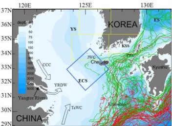
water with deep ocean properties (and perhaps coastal prop-erties) originating from the Kuroshio branching and Taiwan Strait. The peak YR discharge during the late spring-summer results in the low density diluted water that floats over the high salinity oceanic water and thus a plume front develops (Beardsley et al., 1985). In these seasons, the plume spreads eastward over the broad ECS, reaching as far as Jeju Island and the shelf-break, where the Kuroshio flowing northward transports the LSW plume to the northeastern and further eastern region of this Island. This leads to extensive water exchange between the ECS and Kuroshio across the shelf-break through frontal and other oceanic processes. Such a complex situation with a high load of YR discharge strongly influences the optical properties of estuarine surface waters in the spring-summer season.
3 Approach
In this approach,aCDOM (m−1)at 400 nm and 412 nm are
determined in order to describe its absorption as a function of wavelengthλusing a single exponential model in which the spectral slopeS as a proxy for CDOM composition is estimated by the ratio ofaCDOMat 412 nm and 400 nm and
the reference is explained simply byaCDOM at 412 nm. For
derivingaCDOM(400) andaCDOM(412), a simple power-law
formula is chosen because of its good performance over the other formulas, taking advantage of decreased radiance (or reflectance) in the blue (412–490 nm) and increased radiance (or reflectance) in the green (555 nm) by working in terms of the ratios in these two wavelengths. As the absorption by CDOM is strong atλ<500 nm, we seek to evaluate three spectral ratios in the calculation which takes the form,
C=α R
rs(λ1)
Rrs(λ2) −β
, (1)
whereCrepresents the absorption coefficient of CDOM, i.e. aCDOMat 400 nm or 412 nm,αandβare the regression
coef-ficients,λ1=412 nm, 443 nm or 490 nm, andλ2=555 nm, and
Rrsis the remote sensing reflectance. This formula is effec-tive and applies to a wide range of water types considered in various previous studies. Kahru and Mitchell (2001) derived a similar empirical formula of aCDOM (300) from their
in-situ data set, wherein the normalized water-leaving radiance (nLw)ratios nLw(443)/nLw(520) for OCTS (Ocean Colour and Temperature Sensor) and nLw(443)/nLw(510) for SeaW-iFS are used to avoid known problems with atmospheric cor-rection at short wavelengths. However, to produce accurate estimates ofaCDOM(λ)from remotely sensed data, Cullen et
al. (1997) and Johannessen et al. (2003) suggested the use of the blue-green band ratio of remote sensing reflectances (Rrs(412)/Rrs(555)) as a predictor ofaCDOM(λ)throughKd (λ)for the surface layer of the ocean, while others (e.g. Bow-ers et al., 2004; Kutser et al., 2005) proposed the linear or power-law relationships but using the red-green band ratio of
718
Fig. 1. A map showing the study area and sampling grids from where in-situ bio-optical data were collected during the R/V EARDO, Olympic and Tamgu cruises (1998–2005) in the Korean South Sea (KSS, R/V Olympic), Yellow Sea (YS, R/V EARDO and Tamgu) and East China Sea (ECS, R/V EARDO). The yellow and blue colour boxes represent the in-situ measurements of CDOM and salinity along with other optical measurements, respectively. YRDW – Yangtze River Diluted Water, CCC – China Coastal Cur-rent, TaWC – Taiwan Warm CurCur-rent, JWC – Jeju Warm CurCur-rent, TWC – Tsushima Warm Current, Kuroshio Current, ES – East Sea. The current patterns and bathymetry information came from Lie et al. (1998) and Shanmugam et al. (2008).
reflectances (Rrs(λ3)/Rrs(λ2), whereλ3=665 nm or 670 nm
andλ2=490 or 565 nm). It seems that the power-law
relation-ship using the ratio of reflectance or radiance at two visible wavelengths (blue-green) is reasonable to provide reliable es-timates ofaCDOM(λ)from remotely sensed data.
The spectral behavior of the absorption of light by CDOM can be modeled as a function ofλusing a single exponential model which takes the form as below,
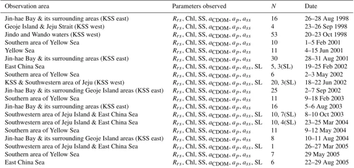
Table 1.Information regarding the in-situ data.N– number of observations, and SL – salinity.
Observation area Parameters observed N Date
Jin-hae Bay & its surrounding areas (KSS east) Rrs, Chl, SS,aCDOM,ap,ass 16 26–28 Aug 1998 Geoje Island & Jeju Strait (KSS west) Rrs, Chl, SS,aCDOM,ap,ass 4 23–26 Sep 1998 Jindo and Wando waters (KSS west) Rrs, Chl, SS,aCDOM,ap,ass 53 20–23 Oct 1998 Southern area of Yellow Sea Rrs, Chl, SS,aCDOM,ap,ass 10 1–5 Feb 2001
Yellow Sea Rrs, Chl, SS,aCDOM,ap,ass 11 4–15 Jun 2001
Jin-hae Bay & its surrounding areas (KSS east) Rrs, Chl, SS,aCDOM,ap,ass 30 28–31 Aug 2001 East China Sea Rrs, Chl, SS,aCDOM,ap,ass, SL 5, 3(SL) 19–25 Feb 2002 Southern area of Yellow Sea Rrs, Chl, SS,aCDOM,ap,ass 6 2–3 May 2002 KSS & Southwestern area of Jeju (KSS west) Rrs, Chl, SS,aCDOM,ap,ass, SL 20, 3(SL) 18–22 Jun 2002 Jin-hae Bay & its surrounding Geoje Island areas (KSS east) Rrs, Chl, SS,aCDOM,ap,ass 25 2–7 Sep 2002 Southern area of Yellow Sea Rrs, Chl, SS,aCDOM,ap,ass 11 9–18 Feb 2003 Jin-hae Bay & its surrounding areas (KSS east) Rrs, Chl, SS,aCDOM,ap,ass 16 5–6 Aug 2003 Southwestern area of Jeju Island & East China Sea Rrs, Chl, SS,aCDOM,ap,ass, SL 10, 7(SL) 8–10 Oct 2003 Southwestern area of Jeju Island & East China Sea Rrs, Chl, SS,aCDOM,ap,ass, SL 10, 4(SL) 23–25 Mar 2004 Southern area of Yellow Sea Rrs, Chl, SS,aCDOM,ap,ass 11 9–12 May 2004 Jin-hae Bay & its surrounding Geoje Island areas (KSS east) Rrs, Chl, SS,aCDOM,ap,ass 8 10–11 Aug 2004 Southwestern area of Jeju Island & East China Sea Rrs, Chl, SS,aCDOM,ap,ass, SL 1 26–27 Mar 2005 Southern area of Yellow Sea Rrs, Chl, SS,aCDOM,ap,ass 7 29 May 2005 East China Sea Rrs, Chl, SS,aCDOM,ap,ass, SL 6 22–29 Aug 2005
water types is considered of interest. Thus, we introduce a method that permits the use of the fixed wavelength ratio of aCDOM (400) andaCDOM(412) for estimating S and
there-fore simplifies the comparison ofS values from CDOM in different environments. The method takes the form
S=
1 λi−λj
×ln
a
CDOM(λi) aCDOM(λj)
, (3)
whereλi andλj are 412 nm and 400 nm and now the above equation becomes
S=
1 12
×ln
a
CDOM(412)
aCDOM(400)
=
1 12
×ln α (Rrs(λ1)/Rrs(λ2))
−β
α (Rrs(λ1)/Rrs(λ2))−β !
, (4)
whereαandβ are the regression coefficients for estimating aCDOM(400) andaCDOM(412) using the reflectance band
ra-tio algorithms. This calculara-tion allows a better estimara-tion of S to distinguish between marine and terrestrial organic matter from measurements of the absorption at two of these wave-lengths.
4 Materials and methods
4.1 Data sets and measurements
Data used in this study were collected from a wide range of water types in the ECS, YS and KSS. Table 1 provides the information on the time and location, and type and number
of measurements, all made within sampling grids illustrated on the regional map in Fig. 1. For each station, remote sens-ing reflectance (Rrs), chlorophyll (Chl), suspended sediment (SS), and absorption coefficients of CDOM (aCDOM),
phy-toplankton (ap)and non-algal particles (ass)of water sam-ples were measured. There were fewer salinity (SL) mea-surements but taken mostly from the YR estuarine, mixing and oceanic regions of the ECS. In what follows the meth-ods of these measurements relevant to this study are briefly described.
4.2 Remote sensing reflectance (Rrs)
For each cruise and at each station, in-situ radiometric mea-surements (above the seawater) were performed in the 350– 1050 nm spectral range (with a 1.4 nm spectral interval) from a calibrated ASD FieldSpec Pro Dual VNIR Spectroradiome-ter. These measurements included the total water leaving ra-diancet Lw(λ), sky radianceLsky(λ)and downwelling
irra-dianceEd(λ). Thet Lw(λ)andLsky(λ)were measured with
a pointing angleθ∼25–30◦from nadir and an azimuthal
an-gleφ∼90◦ from the solar plane, whereas sky radiance was
measured in the same plane ast Lw(λ)but from a direction of θ∼30 from zenith. Ed (λ) was measured by pointing the sensor upward from the deck. Most of these measure-ments were made in excellent conditions, near solar noon and under almost cloudless conditions. Sincet Lw(λ) con-sisted of the desired water-leaving radianceLw(λ)and a con-tamination term1L(=Fr(λ)×Lsky(λ)), it was necessary to
contributions of skylight reflection (Lsky(λ))and Fresnel
re-flectance (Fr(λ))of air-sea interface using,
Lw(λ)=t Lw(λ)−1L. (5)
In the above calculation, the values ofLsky(λ)were obtained
from the sky radiometer, and theFrvalue was assumed to be 0.025 (Austin, 1974). In fact,Frvaries with viewing geome-try, sky conditions and sea surface roughness due to wind and is wavelength-dependent under a cloudy sky (Mobley, 1999). Applying these values in Eq. (5) yielded the water-leaving radiance (Lw(λ)), which was then divided by downwelling irradiance to obtain the remote sensing reflectanceRrs (λ) using,
Rrs(0+λ)=
Lw(λ) Ed(0+λ)
, (6)
where the Rrs(λ), referred in units of sr−1, is an apparent optical property (AOP) that contains the spectral informa-tion of the water-leaving radiance, but which is largely free of its magnitude variability. Thus, algorithms and models have been developed to relateRrs measurements to in-water constituents, such as Chl, SS and CDOM (e.g. O.Reilly et al., 1998; He et al., 2000; Montes-Hugo et al., 2005; Johan-nessen et al., 2003).
4.3 Absorption coefficient of CDOM
Immediately after collection with Niskin bottles, the sam-ples were filtered on board through 0.45µm membrane sy-ringe filters (25 mm), previously rinsed with ultra pure Milli-Q water and 50 ml of the sample were stored in glass flasks in the dark at 4◦C for analysis in laboratory. After return-ing to the laboratory, the absorbance of CDOM was mea-sured between 350–900 nm (with 1 nm increments) using a dual-beam Perkin-Elmer Lambda 19 spectrophotometer. The measurements were performed by placing a 10 cm quartz cu-vette containing Milli-Q water in the optical path of the ref-erence beam, and a 10 cm quartz cuvette containing the fil-tered seawater sample in the optical path of the sample beam. The spectral absorption coefficientaCDOM(λ)was computed
from the measured absorbance resulting from the difference between the sample absorbance and the reference absorbance (Ferrari et al., 1996), from
aCDOM(λ)=
2.3025×ACDOM(λ)
Lc , (7)
whereLcis the path length of the cuvette (i.e. 0.1 in units of meters). TheaCDOM(λ)values measured for a variety of
wa-ter types were generally found to decrease almost exponen-tially throughout the near UV and visible spectral domains (Bricaud et al., 1981; D’Sa et al., 1999).
4.4 Salinity
Salinity measurements data were collected from the conductivity-temperature-depth (CTD) sensors (Sea-Bird
Electronics) during the six R/V EARDO cruises (2002– 2005) in the ECS, southern YS and western Jeju Island. An-other set of salinity data along with theaCDOM(400) (m−1)
measured with a Lambda-18 spectrophotometer from Miller et al. (2002), were also included in our analysis to find an ap-propriate relationship with higher accuracy and apply it to a variety of waters. They collected these data for a wide range of waters in the Bay St. Louis, MS, Lake Pontchartrain, LA, Mississippi Sound, MS, and Mississippi River Delta, MS. The above data sets are a good representative of the rivers, coastal, estuarine, mixing and oceanic regions, and are there-fore used to derive an algorithm for retrieving salinity, which is a primary tracer of the LSW plume around coast and estu-ary.
4.5 Satellite data and processing
Siegel et al. (2002), D’Sa et al. (2002) and Johannessen et al. (2003) have demonstrated that ocean colour data from NASA’s (National Aeronautics and Space Administration) SeaWiFS sensor can be used to derive the products ofaCDOM
400
400 450 500500 550 600600 650 700700 0.0
0.2 0.4 0.6 0.8
400
400 450 500500 550 600600 650 700700 0.0
0.5 1.0 1.5 2.0
aCD
O
M
(
λ
) (m
-1)
Wavelength (nm)
aCD
O
M
(
λ
) (
m
-1 )
Wavelength (nm)
λ Fig. 2.Spectral variations in the absorption coefficient of coloured dissolved organic matter (aCDOM(λ), m−1))in ECS, YS and KSS
waters (N=470). Top panel is from the ECS, YS and also KSS and bottom panel is from the KSS.
For comparison, we also processed some of SeaWiFS im-ages using the SAC algorithm (with SeaDAS version 4.4) and estimatedaCDOM and salinity using the empirical
rela-tionships developed in this study.
5 Results
5.1 Spectral variations of CDOM
Spectral variations of the absorption coefficient of CDOM (aCDOM(λ))are shown in Fig. 2. The general spectral curves
show very low absorption values (<0.163 m−1)at the red portion of the visible spectrum (650 nm), which increase to maximum values according to exponential laws in the near UV/lower blue domains (400–412 nm), as previously reported by Bricaud et al. (1981).aCDOM(412) values were
generally observed to range from 0.05–0.6 m−1in the ECS and YS characterized by Chl 0.4–7.9 mg m−3 and SS 0.5– 68 g m−3, and from 0.9–1.76 m−1 in the KSS characterized by Chl 0.08–119 mg m−3and SS 1.4–260 g m−3. The val-ues higher than 0.9 m−1in the KSS coastal areas may be
re-lated to increased contamination/pollution of waters (bottom panel), and the values lower than 0.3 m−1 in offshore wa-ters of the ECS and YS may be the result of the freshwater influence and local biological activity near the surface layer (top panel). The CDOM measured in the ECS (southwest off Jeju Island) are generally at moderate levels (0.3–0.6 m−1), largely influenced by high fluvial discharges at the mouth of the YR and advection processes at the offshore areas of the YR mouth. Higher magnitudes are often evident toward the ECS coast, particularly during the peak-runoff periods from late spring-summer (Guo et al., 2007; Tang, 2008).
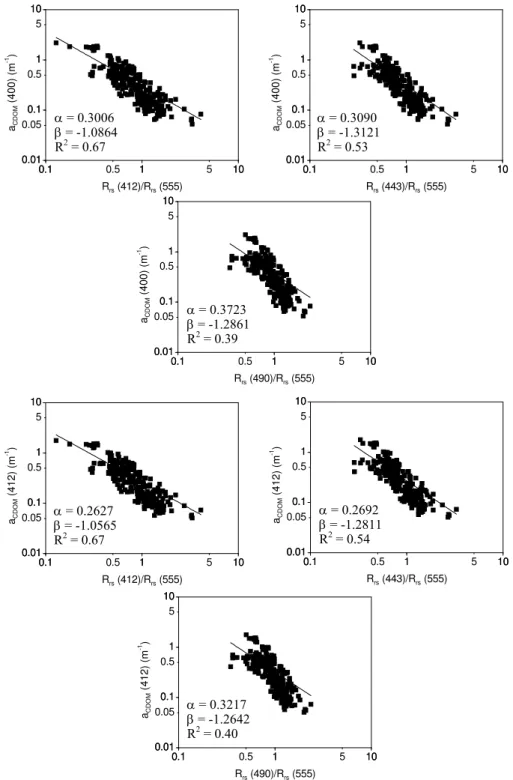
5.2 EstimatingaCDOM(400, 412) from remote sensing
re-flectance (Rrs)
To estimate CDOM absorptions at these two wavelengths, we tried to find the strongest relationship between log-transformed aCDOM (400, 412) and log-transformed three
spectral ratios of the remote sensing reflectance Rrs (412)/Rrs (555), Rrs (443)/Rrs (555) and Rrs (490)/Rrs (555) from our large in-situ bio-optical data set collected in the study regions (Fig. 3 with inclusion of regression coef-ficients). The basic thought behind selecting and examin-ing these band combinations and ratios is that variations in Rrs at the blue wavelengths are strongly affected by CDOM absorption, compared with other light absorbing water con-stituents, and variations inRrsat the green wavelengths are the most affected by light scattering by particles (Johan-nessen et al., 2003; Belanger et al., 2008). Of the three ratios examined, the ratio of reflectance at 412 nm to reflectance at 555 nm allowed one to predictaCDOM (400) andaCDOM
(412) more robustly with the correlation coefficientR2=0.67. As CDOM absorption had a characteristic exponential de-cay with wavelength, it was not well correlated with theRrs (443)/Rrs (555) and Rrs (490)/Rrs (555) ratios, and thus the relationships between these ratios and aCDOM at 400
and 412 nm were weakly consistent (R2=0.53–0.54 forRrs (443)/Rrs (555) vs. aCDOM (400, 412), and R2=0.39–0.40
forRrs (490)/Rrs (555) vs.aCDOM (400, 412), forN=254).
Statistical regression analysis of the former relationships pro-vided the best-fit power function equations with constant co-efficients (Fig. 3) that capture a large fraction of the varia-tion in the reflectance band ratios (Rrs(412)/Rrs(555)) and variation in the aCDOM values (at 400 and 412 nm).
How-ever, this was not the case for the later power models (ofRrs (443)/Rrs (555) and Rrs (490)/Rrs (555) vs. aCDOM (400,
412)) that did not linearly fit the most frequent central and extreme data. This suggests that a wide range of variability in aCDOMis difficult to retrieve from these relationships. Thus,
this study fixes theRrs(412)/Rrs(555) ratio as a predictor of theaCDOMat 400 nm and 412 nm. If the atmospheric
correc-tion of blue band is accurate, then the estimacorrec-tion ofaCDOM
0.1
0.1 0.5 11 5 1010 0.01 0.01 0.05 0.1 0.1 0.5 1 1 5 10 10 0.1
0.1 0.5 11 5 10 0.01 0.01 0.05 0.1 0.1 0.5 1 1 5 10 10 10 0.1
0.1 0.5 11 5 1010 0.01 0.01 0.05 0.1 0.1 0.5 1 1 5 10 10 0.1
0.1 0.5 11 5 1010 0.01 0.01 0.05 0.1 0.1 0.5 1 1 5 10 10 0.1
0.1 0.5 11 5 10 0.01 0.01 0.05 0.1 0.1 0.5 1 1 5 10 10 10 0.1
0.1 0.5 11 5 1010 0.01 0.01 0.05 0.1 0.1 0.5 1 1 5 10 10 aCDO M (40 0 ) (m -1 )
Rrs (412)/Rrs (555)
aCDO M (40 0 ) (m -1 )
Rrs (443)/Rrs (555)
aCDO M (40 0 ) (m -1 )
Rrs (490)/Rrs (555)
aCDO M ( 4 12 ) (m -1 )
Rrs (412)/Rrs (555)
aCDO M (41 2 ) (m -1 )
Rrs (443)/Rrs (555)
aCDO M ( 4 12 ) (m -1 )
Rrs (490)/Rrs (555)
α = 0.3006 β = -1.0864 R2 = 0.67
α= 0.3090 β = -1.3121 R2 = 0.53
α= 0.3723 β = -1.2861 R2 = 0.39
α= 0.2692 β = -1.2811 R2 = 0.54
α= 0.3217 β = -1.2642 R2 = 0.40 α = 0.2627
β = -1.0565 R2 = 0.67
Fig. 3.Relationships between the threeRrsratios andaCDOM(400, 412) (m−1)measured (in-situ) in a wide range of waters from the ECS,
YS and KSS during 1998–2005 (N=254).
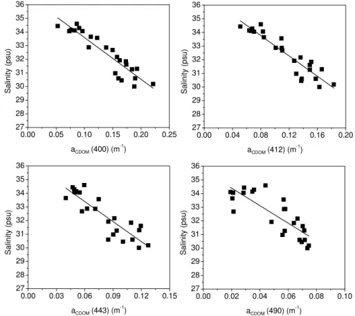
5.3 Relationship between salinity andaCDOM(λ)
As the salinity has no direct colour signal, it could be rather estimated through the colour signal dominated by major wa-ter constituents, such as the CDOM (Moon et al., 2006; Del Castillo and Miller, 2008). Thus, this study was to
exam-ine the relationships between salinity and absorption coeffi-cient of CDOM measured in estuarine and offshore waters of the ECS. Figure 4 displays the scatter plots of salinity ver-sus aCDOM at 400 nm, 412 nm 443 nm and 490 nm (m−1),
wherein tight, inverse relationships of salinity andaCDOM(λ)
0.00 0.05 0.10 0.15 0.20 0.25 27
28 29 30 31 32 33 34 35 36
0.00 0.04 0.08 0.12 0.16 0.20 27
28 29 30 31 32 33 34 35 36
0.00 0.03 0.06 0.09 0.12 0.15 27
28 29 30 31 32 33 34 35 36
0.00 0.02 0.04 0.06 0.08 0.10 27
28 29 30 31 32 33 34 35 36
Sa
lin
ity (
p
su
)
aCDOM (400) (m -1
)
Sa
lin
ity (
p
su
)
aCDOM (412) (m -1
)
Sa
lin
ity (
p
su
)
aCDOM (443) (m -1
)
Salin
it
y
(
p
s
u
)
aCDOM (490) (m -1
)
λ
Fig. 4.Relationships between the salinity andaCDOM(λ)(m−1)observed in estuarine and offshore waters of the ECS during 2002–2005 (N=24).
Table 2. Parameters for the estimation of salinity (psu) from the
aCDOM(λ).
Algorithms aCDOM(λ) A B R2 N
Salinity aCDOM(400) −30.6416 36.6551 0.86 24 Salinity aCDOM(412) −37.3089 36.7550 0.85 24 Salinity aCDOM(443) −48.9630 36.3301 0.77 24 Salinity aCDOM(490) −64.4025 35.6943 0.66 24 Salinity aCDOM(400) 35.064 −0.3357 0.98 37
that decreased from 0.86–0.66 with CDOM absorption at the increased wavelengths. Linear regression of the salinity per-formed againstaCDOM(λ)data was found quite appropriate
for this data, yielding approximately the following expres-sion,
Salinity (psu)=A×aCDOM(λ)+B, (8)
whereAandB are the regression coefficients given in Ta-ble 2. As a consequence of its fresh water origin and conser-vative behavior, CDOM absorption in coastal seas has been previously observed to be inversely correlated with salinity in
the same way, and therefore has been considered a good indi-cator of salinity in various regions (e.g. Jerlov, 1968; Nelson and Guarda, 1995; Boss et al., 2001; Binding and Bowers, 2003; Kwalczuk et al., 2005; Moon et al., 2006; Guo et al., 2007; Sasaki et al., 2008). Findings from the above relation-ships of salinity andaCDOM(λ)revealed that salinity seemed
to be better correlated with aCDOM at 400 nm thanaCDOM
at other longer wavelengths, and thereforeaCDOMat 400 nm
could be used as a proxy for salinity in this region.
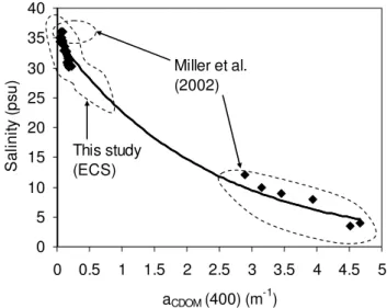
Since our data were determined by the ranges of 30–34.4 (psu) salinity and 0.05–0.22 (m−1) aCDOM (400), it was
quite difficult to find a more appropriate relationship between salinity andaCDOM(400) and apply it to satellite data to infer
salinity in a variety of water types commonly observed in the riverine-estuarine systems. By adding the data of Miller et al. (2002), we found that the salinity was highly inversely correlated (R2=0.98) with aCDOM (400), with a
substan-tial positive intercept, and this correlation corresponded best with an exponential rather than a linear function ofaCDOM
(400) measured in waters of the ECS (Fig. 5). The best-fit exponential curve (with the smallest error of slope, 0.03) for a variety of samples can be approximated by
with the more reliable regression coefficients described in Ta-ble 2. It was noted that the variability in CDOM concentra-tion within waters of low salinity 2.5–12 psu (when consider-ing all data from Miller et al., 2002) was slightly larger than that found in waters of high salinity 30–34.4 psu (ECS). This may be due to the higher CDOM concentration/variability in riverine inputs and accumulation of CDOM from in-water productivity and/or sediment-released CDOM into the re-gions studied by Miller et al. (2002). This trend of variabil-ity in waters of high CDOM concentration and low salinvariabil-ity has been reported in several earlier investigations of similar environments (Vodacek et al., 1997; Boss et al., 2001; Twar-dowski and Donaghay, 2001; Guo et al., 2007). Binding and Bowers (2003) pointed out that a part of such variability may also occur both geographically and temporally with factors such as variations in the availability and type of organic mat-ter, volume and persistence of rainfall, and size of catchment area. However, the existence of the tight, inverse relation-ship between salinity andaCDOM(400) for a variety of
sam-ples from different seasons and from a variety of water types, implies that the salinity variation around the mouth and estu-ary of the YR can be accurately estimated if products of the CDOM absorption are assured by the atmospheric correction scheme applied to satellite data.
5.4 Validation ofaCDOM(400) and salinity retrievals
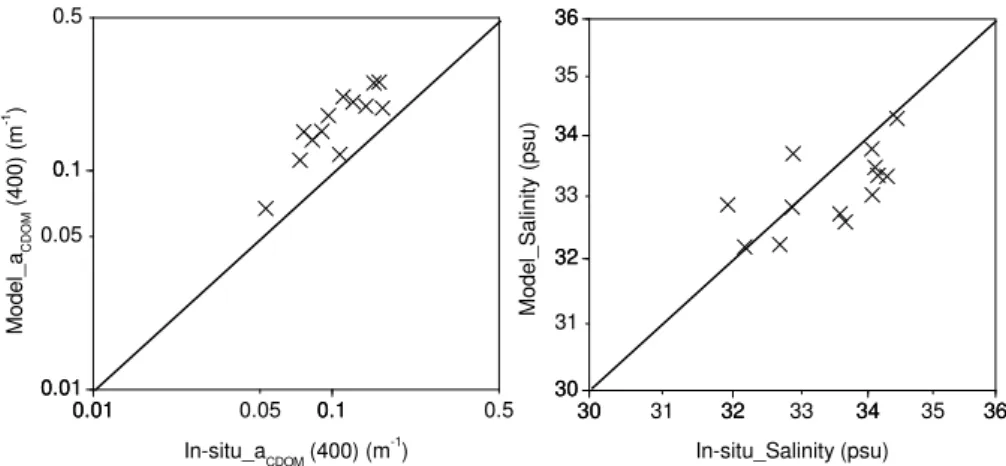
We applied the respective relationships (in Figs. 3 and 5, Ta-ble 2) to our in-situRrs data (from spring–summer 2002– 2005) and compared the model estimates of aCDOM (400)
(m−1)and salinity (psu) with those from shipboard measure-ments obtained in estuarine mixing and oceanic waters of the ECS (Fig. 6). Although the data set used for this validation contains only 13 in-situ measurements, it provides a better idea about the overall performance of these models for esti-matingaCDOM(400) and salinity in the LSW plume region of
the ECS. It appears that theaCDOM(400) values are closely
linearly aligned around the 1:1 line, although slightly higher than the in-situaCDOM(400) values. The overestimation is
particularly more pronounced for highly turbid waters with aCDOM (400) >0.5 m−1 and less pronounced for relatively
clear waters withaCDOM (400) <0.1 m−1. However, LSW
plume containsaCDOM (400) values typically ranging from
0.08–0.4 m−1toward the ECS coast and 0.05–0.25 m−1 to-ward the estuarine mixing waters offshore of the mouth of the YR (Moon et al., 2007; Tang, 2008). As a result, the model performance is found to be quite satisfactory with the mean relative error MRE 0.58 (= modelaCDOM(400) –
in-situaCDOM (400)/in-situ aCDOM (400)) and correlation
co-efficientR2 0.71. On the other hand, the comparison be-tween modeled and measured salinity shows good agree-ment (MRE=−0.009, R2=0.41), but with increased scatter of matches underlying the regression line in Fig. 6 (plot on the right side). This suggests slight uncertainty in salinity retrievals which may be associated with errors in model
es-0 5 10 15 20 25 30 35 40
0 0.5 1 1.5 2 2.5 3 3.5 4 4.5 5
aCDOM (400) (m -1
)
Sa
lin
it
y
(
p
s
u
)
This study (ECS)
Miller et al. (2002)
Fig. 5.Relationship between the salinity andaCDOM(400) (m−1)
measured in a diverse range of waters from the ECS and other re-gions (N=37).
timates of theaCDOM(400) from in-situRrsdata. Neverthe-less, the nonlinear exponential relationship would achieve a relatively higher accuracy (±1 psu) for estimating salinity in comparison with other linear models previously developed for this region (Sasaki et al., 2008).
5.5 Implementation to SeaWiFS ocean colour imagery The relationships obtained in this study were implemented together with the regional atmospheric correction algorithm (SSMM) to a series of SeaWiFS images of the springtime (1998–2005, no reliable cloud free images available for April–May in 2000 and 2002) for mapping and monitoring the LSW plume in the YR estuary and coastal areas of the ECS, where conservative behavior of CDOM during estuar-ine mixing and CCC waters has been reported in the previous shipboard or satellite-based observations (Ahn et al., 2004; Guo et al., 2007). Figures 7 and 8 show persistent patches of aCDOM (400) associated with the LSW plume,
coincid-ing with the broad continental shelf of the 50 m isobath east of the YR mouth and south/west of the YS. It is interest-ing to note that aCDOM (400) is seen to be typically below
0.15 m−1 in Kuroshio waters and varies from 0.15 m−1 in YS/offshore waters to 0.4 m−1in YRDW waters formed by mixing between the YR runoff and saline waters south/west of the YS. A pronounced CDOM maximum is found within regions of the concentrated fresh water runoff and around the mouth of the YR, whereaCDOM(400) reaches 0.5 m−1.
878 879 880 881 882 883 884 885 886 887 888 889
30
30 31 3232 33 3434 35 3636 30
30 31 32 32 33 34 34 35 36 36
0.01
0.01 0.05 0.10.1 0.5 0.01
0.01 0.05 0.1 0.1 0.5
M
o
del_S
a
lini
ty
(ps
u
)
In-situ_Salinity (psu)
Mo
del
_a
CDO
M
(400)
(m
-1 )
In-situ_aCDOM (400) (m-1)
Fig. 6. Comparison of modeledaCDOM(400) (m−1)and salinity (psu) with those from shipboard measurements (in-situ) obtained in the
ECS during spring–summer 2002–2005 (N=13).
aCDOM (400) aCDOM(400)
7 April 1999 27 April 1998
aCDOM (400)
10 May 2001
aCDOM(400)
2 May 2003
aCDOM (400)
28 April 2004
aCDOM(400)
5 April 2005
Fig. 7.Maps derived from the SeaWiFS images showing the springtime distribution of coloured dissolved organic matter (aCDOMat 400 nm,
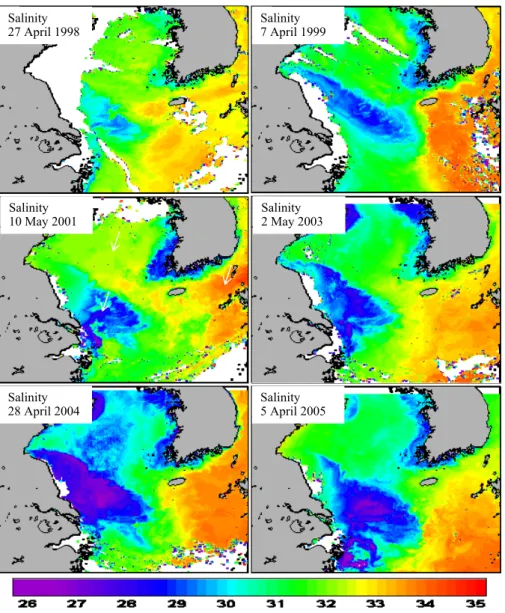
Salinity 2 May 2003 Salinity
27 April 1998
Salinity 7 April 1999
Salinity 10 May 2001
Salinity 28 April 2004
Salinity 5 April 2005
Fig. 8.Maps derived from the SeaWiFS images showing the springtime evolution of salinity fields (psu) in the ECS, YS and KSS. SSMM atmospheric correction was applied to process these images.
ECS through the Tsushima Strait in the northwest and Tokara Strait in the south of Kyushu (Feng et al., 2000); moder-ate salinities (30–32 psu) are often observed in the YS where these values go up to 34 psu when the Yellow Sea Warm Cur-rent (YSWC) as a breach of Kuroshio intrudes into the south-ern YS northwest off the Jeju Island (Lie and Cho, 2002); minimum salinities are noticed around YRDW (28.5–30 psu) and mouth of the YR (26.5–28.5 psu). SeaWiFS-derived salinity images also reveal the source and extent of these low salinity waters that appear to be displaced north of the YR mouth and adopt a nearly linear pattern corresponding with the broad ECS shelf (7 April 1999 as a good example). These results are closely consistent with previous shipboard observations of the surface salinity in the ECS and model-ing studies (Chen at al., 2006, 2008). The contributions of high CDOM concentrations and hence lower salinities are
also noted on occasions in the central part of the YS because of the seaward spreading of the LSW plume during the late April–summer (e.g. 28 April 2004).
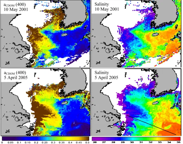
aCDOM (400) 5 April 2005
Salinity 10 May 2001 aCDOM (400)
10 May 2001
Salinity 5 April 2005
Fig. 9. SeaWiFS images of coloured dissolved organic matter (aCDOMat 400 nm (m−1))and salinity (psu) for 10 May 2001 and 5 April
2005. Standard atmospheric correction (SAC) was applied to process these images.
spring–summer season. The 10 May 2001 image is a good example to show how the YR greatly influences the colour of the ECS where highaCDOM(400) (0.5 m−1)abundances
emerging from the southern channel of the YR appear to move northward, then eastward and finally spread out to the shelf area with varying salinities 27–30 psu. This pattern may be influenced by the TaWC which flows northward steadily in this period, carrying water with deep ocean and coastal properties originating from the Kuroshio branching and Tai-wan Strait (elevated CDOM concentrations, 0.25–0.3 m−1, in the 10 May 2001 image).
To assess how reliable these products are when using the standard atmospheric correction (SAC) algorithm for oper-ational mapping and monitoring of the LSW plume in the ECS, two of the above SeaWiFS images acquired on 10 May 2001 and 5 April 2005 were processed using the SAC algo-rithm and estimates ofaCDOM(400) (m−1)and salinity (psu)
were obtained using the same relationships applied before (Fig. 9). Although the SAC algorithm tended to produce re-alistic estimates ofaCDOM(400) and salinity in the Kuroshio
Current region (offshore), it showed large errors (aCDOM
at 400>10 m−1, and salinity<10 psu) around the edges of clouds/aerosols and masked out the entire nearshore areas.
This resulted in the reduced areal coverage withaCDOM(400)
and salinity fields within estuary and coastal areas. The cause of such errors associated with the SAC algorithm could be at-tributed to the nearly zero and improbable negativeRrs val-ues that occurred as a result of excessive aerosol path radi-ance removal in the visible bands due to the overestimated ε=ρas(765)/ρas(865)in highly turbid and productive waters (McClain et al., 2000; Shanmugam and Ahn, 2007). Such problems were actually manifested in negative nLw values obtained from MODIS images using the SAC algorithm, ul-timately causing an inaccuracy in the satellite estimates of aCDOM(400) and salinity, and thus preventing their potential
applications for mapping and monitoring the LSW plume in the ECS (Sasaki et al., 2008). Avoiding these problems by using a cutoff value of nLwwould, on the other hand, elim-inate a large number of the useful pixels toward the estuary and coast from where the LSW plume starts to dominate the colour of the ECS (Sasaki et al., 2008).
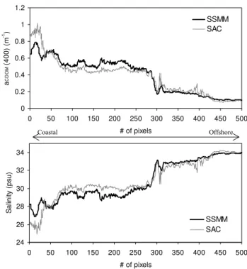
Figure 10 allows one to closely examine the spatial vari-ability ofaCDOM(400) and salinity along a transect running
comparison of these properties showed that the agreement of SeaWiFS-SAC retrievals ofaCDOM(400) and salinity was
stronger in the Kuroshio Current region where these values approached 0.1 m−1 (and even below) and 34 psu, respec-tively. However, extending comparisons from offshore to-ward the estuary area revealed thataCDOM(400) and salinity
distributions inferred from these two atmospheric correction schemes significantly differed when delivery by the YR and CCC during 5 April 2005 affected theaCDOM (400) values
greater than 0.6 m−1 and salinity lower than 28 psu. This results in large errors whenaCDOM (400) is>0.8 m−1 and
salinity is<26 psu, delivered by the SAC algorithm. Never-theless, there was good consistency between these two atmo-spheric correction algorithms over relatively clear regions, with a mean difference of 0.009 inaCDOM(400) (m−1)and
0.096 in salinity (psu).
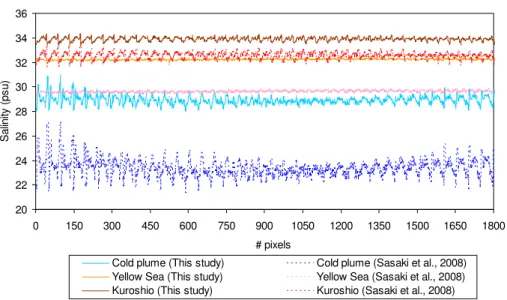
In addition, we also assessed the performance of our non-linear salinity model (NLSM) in comparison with the results of the linear salinity model (LSM) developed by Sasaki et al. (2008) and in-situ observations of Chen et al. (2006) and NFRDI (http://www.nfrdi.re.kr/page?id=kr index). We ap-plied these two models to the SeaWiFS image of 10 May 2001 and compared the predicted salinities around the LSW plume, YS and Kuroshio (arrow marks on the salinity im-age of 10 May 2001 in Fig. 8). It is important to note that salinity estimations from the NLSM substantially differed with those from the LSM in these three water types, being closely consistent with in-situ observations made by Chen et al. (2006) and NFRDI during the spring (Fig. 11; Table 3). In contrast, salinities predicted by the LSM were always lower than those predicted by the NLSM and observed by Chen et al. (2006) and NFRDI, and this underestimation was the largest from warmer Kuroshio toward colder YR estuary waters: i.e. 1.4 psu in the Kuroshio, 2.8 psu in the YS and 5.6 psu in the LSW plume regions. This discrepancy was likely caused by the LSM because it was derived from the limited number of salinity and CDOM data collected from the restricted range of waters offshore of the ECS. The un-derestimation was also manifested in their satellite-derived salinity from the LSM at several locations (including the ar-eas affected by aerosols and clouds) and was partly attributed to by the problems of atmospheric correction in these waters. 5.6 Nature of the CDOM pool
To identify the nature of the CDOM pool, we applied Eqs. (3) and (4) to the SeaWiFS image of 10 May 2001 for produc-ing an image of the areal distribution of CDOM absorption slope coefficient (a proxy for changes in the CDOM compo-sition) in the ECS. The slope coefficients calculated using the aCDOM at 400 nm and 412 nm were generally in good
agreement with measured values at various stations in the ECS and in waters of other similar environments (Bricaud et al., 1981; Davies-Colley, 1992; Green and Blough, 1994; Kowalczuk et al., 2005). This coefficient, largely
indepen-24 26 28 30 32 34
0 50 100 150 200 250 300 350 400 450 # of pixels
S
a
lin
ity
(
p
s
u
)
500 SSMM SAC 0
0.2 0.4 0.6 0.8 1 1.2
0 50 100 150 200 250 300 350 400 450 # of pixels
a
CD
O
M
(
400)
(
m
-1)
500 SSMM SAC
Offshore Coastal
Fig. 10. Horizontal profiles from the SeaWiFS image of 5 April 2005 illustrating the spatial variability ofaCDOM(400) (m−1)and
salinity (psu) fields along a transect running across the LSW plume from bright coastal waters in the YR estuary to dark ocean waters in the vicinity of the Kuroshio (black line on the salinity image in Fig. 9). SAC – standard atmospheric correction scheme, and SSMM – spectral shape matching method scheme.
dent of wavelength, varied from about−0.007 nm−1in clear oceanic waters offshore to −0.016 nm−1 in highly turbid (CDOM-dominated) waters around the mouth and estuary of the YR. This trend of the increased slope coefficient in offshore waters (due to photobleacing) and decreased slope coefficient (due to the terrestrial CDOM pool) in coastal wa-ters is consistent with that inferred from the SeaWiFS ob-servations in the Georgia Bight (Johannessen et al., 2003), suggesting that the methods presented in Eqs. (3) and (4) predict changes in the CDOM composition in ECS waters. By examining the areal distribution of the slope coefficient in Fig. 12, it is clear that the patterns of riverine and ma-rine CDOM pools are well distinguished by high aCDOM
(400) (>0.4 m−1) with low slope values (<−0.15 nm−1) and lowaCDOM (400) (<0.15 m−1)with high slope values
(>−0.015 nm−1), respectively.
6 Discussion and conclusion
+ ×
−
= −
20 22 24 26 28 30 32 34 36
0 150 300 450 600 750 900 1050 1200 1350 1500 1650 1800 # pixels
Sa
lin
ity
(p
s
u
)
Cold plume (This study) Cold plume (Sasaki et al., 2008) Yellow Sea (This study) Yellow Sea (Sasaki et al., 2008) Kuroshio (This study) Kuroshio (Sasaki et al., 2008)
Fig. 11.Comparison of salinity estimations from the nonlinear model (this study) and linear model (proposed by Sasaki et al., 2008) applied to SeaWiFS image of 10 May 2001 at three water types (YR estuary, YS and Kuroshio waters). Mean salinity from the NLSM is 28.9 psu in the LSW plume, 32.2 psu in the YS, and 33.9 psu in the Kuroshio region, whereas mean salinity from the LSM is 23.3 psu in the LSW plume, 29.4 psu in the YS, and 32.5 psu in the Kuroshio region. The linear model is expressed as: Salinity (psu)=−19.5×aCDOM(400) (m−1)+34.5
(withR2=0.66 andN=43).
Table 3.Seasonal average of the YR discharge (m3s−1)and salinity (psu) derived from in-situ observations during 1991–2000 (Chen et al., 2006; NFRDI observations).
Periods YR Salinity Salinity Salinity at
discharge at LSW plume at YS Kuroshio
Spring (March–May) 25 417 31 32 34
Summer (June–August) 50 557 28 31 34
Fall (September–November) 31 520 32 32 34
Winter (December–February) 14 006 31.5 32 34
reactions in the low transparency YR estuary caused by high suspended particulate matter associated with the vertical mixing and riverine/estuarine processes (Guo et al., 2007). Previous studies noted that the magnitude of CDOM absorp-tion is related to variaabsorp-tions in the salinity of the LSW plume generated by coupled YR and CCC systems, where the slope coefficient increases with salinity at high salinity region (29– 31 psu) of the YR estuary (Moon et al., 2006, 2007; Guo et al., 2007). Such behavior and properties within this region could be synoptically mapped and used with other oceano-graphic parameters to understand the dynamics of the out-flowing plume of freshwater which carries loads of particu-late and dissolved substances onto the continental shelf and slope downstream side of Korea, where they strongly influ-ence the colour of the ocean signal recorded by satellite sen-sors.
Satellite remote sensing offers the environmental commu-nity a tool that can synoptically monitor coastal waters at
the accuracy of salinity retrievals from the satellite data. For example, this was particularly apparent in the recent study of the CDOM and salinity variability around the LSW plume re-gion of the ECS using MODIS imagery (Sasaki et al., 2008), whereas their estimates of aCDOM (400) and salinity were
partly or fully disputed at many locations around the edges of clouds and aerosols as being caused by errors due to the atmospheric correction algorithm. Moreover, salinity pre-dicted by their linear model was also significantly underesti-mated within the LSW plume region.
Using our regional in-situ data set of the inherent and ap-parent optical properties (i.e. Rrs and aCDOM), we
estab-lished the empirical relationships in this study for remotely estimating CDOM absorption and salinity within the LSW plume region of the ECS. These relationships were validated with in-situ data and the errors were relatively small and ac-ceptable for remote sensing of the LSW plume in the ECS. When applied together with the SSMM, they particularly provide better estimates of aCDOM (400) and salinity than
the standard algorithms. It should be noted that while these empirical algorithms appear to work satisfactorily in this re-gion, one should be cautious when applying them to other regions where the results would be biased by the influence of high concentrations of chlorophyll/suspended sediments or other properties. This is because the empirical coefficients were derived using a relatively small data set obtained in coastal and estuarine waters with significant terrestrial in-put and should be changed based on measurements from a wide range of waters with different environments. Neverthe-less, we believe that the accuracy of salinity retrievals may be better with the nonlinear model using CDOM absorption at a shorter wavelength (400 nm) where in-water constituents other than CDOM would have a minimal effect. Thus, it may be likely that the salinity retrievals by this model may show success in other regions under the condition that the atmo-spheric correction is fully valid.
Because there appears to be reasonable consistency in the shape of the CDOM absorption spectrum in the near UV and visible regions in a wide range of natural waters (Twardowski et al., 2004), a single spectral shape of the CDOM absorp-tion (in the blue) derived from the remotely sensed signals at two wavelengths allows the proposed exponential model to predict the spectral behavior of CDOM absorption that is needed for a variety of remote sensing applications and bio-optical models. The spectral behavior is indeed largely determined by the slope coefficient as a proxy for CDOM composition. In this paper, we have shown that the slope co-efficients calculated from the ratio ofaCDOM at 400 nm and
412 nm provide the potential for detecting and characterizing the CDOM composition in both coastal and offshore waters of the ECS, where lower slope values corresponded to the ter-restrial pool of CDOM resulting from the rivers and runoff, and higher slope values corresponded to the marine pool of CDOM resulting from the heterotrophic processes near the surface. The estimated coefficients were found to be in good
SeaWiFS Image (10 May 2001)
Fig. 12.Slope coefficient (“S” in nm−1)of the CDOM absorption spectra estimated from SeaWiFS remote sensing reflectance data (10 May 2001) in the ECS.
agreement with the measured values at various stations in the ECS and in waters of other similar environments (Bricaud et al., 1981; Davies-Colley, 1992; Green and Blough, 1994; Kowalczuk et al., 2005).
In conclusion, this paper examined the feasibility of satel-lite remote sensing to assess CDOM and salinity, and thus provides great potential in advancing our knowledge of the shelf-slope evolution and migration of LSW plume in the ECS. As CDOM had the strongest influence on the wa-ter colour signal and perhaps exhibited significantly smaller time and spatial variability compared with the other in-water constituents, we considered it as a potential for mapping and monitoring the LSW plume in the ECS. The salinity was the bi-product ofaCDOM (400) used for better analysis and
in-terpretation of the LSW plume in both coastal and offshore waters. These analyses showed that the variation and extent of the LSW plume were clearly distinguishable within the re-gions of YR river discharge and CCC water using SeaWiFS image data. After the development, the LSW plume was seen to be advected eastward by the influence of the YRDW and TaWC, affecting the shelf-slope waters downstream side of Korea. Thus, this study has led to a better understanding of the spatial and temporal variability with the LSW plume dur-ing the sprdur-ingtime and would be helpful to address several of the environmental and oceanographic issues associated with its evolution and migration in the shelf-slope waters of the ECS.
Topical Editor S. Gulev thanks one anonymous referee for her/his help in evaluating this paper.
References
Ahn, Y. H., Shanmugam., and Gallegos, S.: Evolution of suspended sediment patterns in the East and Yellow Seas, J. Korean Soc. Oceanogr., 39, 26–34, 2004.
Ahn, Y. H. and Shanmugam, P.: New methods for correcting the atmospheric effects in Landsat imagery over turbid (Case-2) wa-ters, Korean J. Rem. Sens., 20, 289–305, 2004.
Austin, R. W.: Inherent spectral radiance signatures of the ocean surface, in: Ocean colour analysis Scripps Institute of Oceanog-raphy, La Jolla, CA, 1974.
Beardsely, R. C., Limeburner, R., Yu, H., and Cannon, G. A.: Dis-charge of the Changjiang (Yangtze River) into the East China Sea, Cont. Shelf Res., 4, 57–76, 1985.
Belanger, S., Babin, M., and Larouche, P.: An empirical algorithm for estimating the contribution of chromophoric dissolved or-ganic matter to total light absorption in optically complex waters, J. Geophys. Res., 113, C04027, doi:10.1029/2007JC004436, 2008.
Binding, C. E. and Bowers, D. G.: Measuring the salinity of the Clyde Sea from remotely sensed ocean colour, Estuarine, Coastal Shelf Sci., 57, 605–611, 2003.
Bowers, D. G., Harker, G. E. L., Smith, P. S. D., and Tett, P.: Optical properties of a region of freshwater influence (the Clyde Sea), Estuarine, Coastal Shelf Sci., 50, 717–726, 2000.
Bowers, D. G., Evans, D., Thomas, D. N., Ellis, K., and Williams, P. J. B.: Interpreting the colour of an estuary, Estuarine, Coastal Shelf Sci., 59, 13–20, 2004.
Boss, E., Pegau, W. S., Zaneveld, R. V., and Barnard, A. H.: Spatial and temporal variability of absorption by dissolved material at a continental shelf, J. Geophys. Res., 106, 9499–9507, 2001. Bricaud, A., Morel, A., and Prieur, L.: Absorption by dissolved
organic matter of the sea (yellow substance) in the UV and visible domains, Limnol. Oceanogr., 26, 43–53, 1981.
Carder, K. L., Chen, F. R., Lee, Z. P., and Hawes, S. K.: Semi-analytic Moderate-Resolution Imaging Spectrometer algorithms for chlorophyllaand absorption with bio-optical domains based on nitrate depletion temperatures, J. Geophys. Res., 104, 5403– 5421, 1999.
Chen, C., Zhu, J., Beardsley, R. C., and Franks, P. J. S.: Physical-biological sources for dense algal blooms near the Changjiang River, Geophys. Res. Lett., 30(10), 1515, doi:10.1029/2002GL016391, 2003.
Chen, X., Wang, X., and Guo, J.: Seasonal variability of the sea surface salinity in the East China Sea during 1990–2002, J. Geo-phys. Res., 111, C05008, doi:10.1029/2005JC003078, 2006. Chen, C., Xue, P., Ding, P., Beardsley, R. C., Xu, Q., Mao, X.,
Gao, G., Qi, J., Li, C., Lin, H., Cowles, G., and Shi, M.: Physi-cal mechanisms for the offshore detachment of the Changjiang Diluted Water in the East China Sea, J. Geophys. Res., 113, C02002, doi:10.1029/2006JC003994, 2008.
Cheng, M. T., Lin, Y. C., Chio, C. P., Wang, C. F., and Kuo, C. Y.: Characteristics of aerosols collected in central Taiwan during an Asian dust event in spring 2000, Chemosphere, 61, 1439–1450, 2005.
Chester, R.: Marine geochemistry, 698 pp., London, Unwin Hyman Ltd, 1990.
Cullen, J. J., Davis, R. F., Bartlett, J. S., and Miller, W. L.: Toward remote sensing of UV attenuation, photochemical fluxes and bi-ological effects in surface waters, Proc. 1997 Aquatic Sciences Meeting, Santa Fe, NM, USA, ASLO, 1997.
Davies-Colley, R. J.: Yellow substance in coastal and marine waters around the South Island, New Zealand, N.Z., J. Mar. Freshwater Res., 26, 311–322, 1992.
Del Castillo, C. E. and Miller, R. L.: On the use of ocean colour remote sensing to measure the transport of dissolved organic car-bon by the Mississippi River Plume, Rem. Sens. Environ., 112, 836–844, 2008.
Doxaran, D., Cherukuru, R. C. N., and Lavender, S. J.: Use of re-flectance band ratios to estimate suspended and dissolved matter concentrations in estuarine waters, Int. J. Rem. Sens., 26, 1763– 1769, 2005.
D’Sa, J. D., Steward, R. G., Vodacek, A., Blough, N. V., and Phin-ney, D.: Determining optical absorption of coloured dissolved or-ganic matter in seawater with a liquid capillary waveguide, Lim-nol. Oceanogr., 44, 1142–1148, 1999.
D’Sa, E. J. D., Hu, C., Muller-Karger, F. E., and Carder, K. L.: Es-timation of coloured dissolved organic matter and salinity fields in case 2 waters using SeaWiFS: Examples from Florida Bay and Florida Shelf, Proc. Indian Acad. Sci. (Earth Planet. Sci.), 111, 197–207, 2002.
Feng, M., Mitsudera, H., and Yoshikawa, Y.: Structure and variabil-ity of the Kuroshio Current in Tokara Strait, Phys. Oceanogr., 30, 2257–2276, 2000.
Ferrari, G. M., Dowell, M. D., Grossi, S., and Targa, C.: Relation-ship between the optical properties of chromophoric dissolved organic matter and total concentration of dissolved organic car-bon in the southern Baltic Sea region, Mar. Chem., 55, 299–316, 1996.
Green, S. A. and Blough, N. V.: Optical absorption and fluorescence properties of chromophoric dissolved organic matter in natural waters, Limnol. Oceanogr., 39, 1903–1916, 1994.
Guo, W., Stedmon, C. A., Han, Y., Wu, F., Yu, X., and Hu, M.: The conservative and non-conservative behavior of chro-mophoric dissolved organic mater in Chinese estuarine waters, Mar. Chem., 107, 357–366, 2007.
He, M. X., Liu, Z. S., Du, K. P., Li, L. P., Chen, R., Carder, K. L, and Lee, Z. P.: Retrieval of chlorophyll from remote-sensing re-flectance in the China Seas, Appl. Optics, 39, 2467–2474, 2000. Hooker, S. B., Firestone, E.., and Acker, J. C.: SeaWiFS Pre-launch Radiometric Calibration and Spectral Characterization, SeaWiFS technical report series, NASA Technical Memorandum 104566, vol. 23, NASA-GFSC, Greenbelt, Maryland, USA, 1994. Jerlov, N. G.: Optical oceanography, Amsterdam, Elsevier, 1968. Johannessen, S. C., Miller, W. L., and Cullen, J. J.: Calculation of
UV attenuation and coloured dissolved organic matter absorption spectra from measurements of ocean colour, J. Geophys. Res., 108, C9, doi:10.1029/2000JC000514, 2003.
Kahru, M. and Mitchell, B. G.: Seasonal and nonseasonal vari-ability of satellite-derived chlorophyll and coloured dissolved or-ganic matter concentration in the California Current, J. Geophys. Res., 106, 2517–2529, 2001.
(CDOM) absorption and apparent optical properties in Baltic Sea waters, Int. J. Rem. Sens., 26, 345–370, 2005.
Kutser, T., Pierson, D. C., Kallio, K. Y., Reinart, A., and Sobek, S.: Mapping lake CDOM by satellite remote sensing, Rem. Sens. Environ., 94, 535–540, 2005.
Lie, H. J., Cho, C. H., Lee, J. H., Niiler, P., and Hu, J. H.: Separation of the Kuroshio water and its penetration onto the continental shelf west of Kyushu, J. Geophys. Res., 103, 2963–2976, 1998. Lie, H. J. and Cho, C. H.: Recent advances in understanding the
circulation and hydrography of the East China Sea, Fisheries Oceanogr., 11, 318–328, 2002.
McClain, C. R., Ainsworth, E. J., Barnes, R. A., Eplee, R. E., Patt, F. S., Robinson, W. D., Wang, and Bailey, S. W.: SeaWiFS post-launch calibration and validation analyses, Part 1, vol. 9, edited by: Hooker, S. B. and Firestone, E. R., NASA Tech. Memo., 2000-206892(2), 82 pp, 2000.
Miller, R. L., Belz, M., Castillo, C. D., and Trzaska, R.: Determin-ing CDOM absorption spectra in diverse coastal environments using a multiple pathlength, liquid core waveguide system, Cont. Shelf Res., 22, 1301–1310, 2002.
Mobley, C. D.: Estimation of the remote sensing reflectance from above-sea surface, Appl. Optics, 38, 7442–7455, 1999.
Monahan, E. C. and Pybus, M. J.: Colour, UV absorbance and salin-ity of the surface waters of the west coast of Ireland, Nature, 274, 782–784, 1978.
Montes-Hugo, M. A., Carder, K. L., Foy, R. J., Cannizzaro, J., Brown, E., and Pegau, S.: Estimating phytoplankton biomass in coastal waters of Alaska using airborne remote sensing, Rem. Sens. Environ., 98, 481–493, 2005.
Moon, J. E., Yang, C. S., and Ahn, Y. H.: Salinity estimation based on inherent optical property (IOP) in the southern Yellow Sea and northern East China Sea, Proc. 4th JKWOC meeting, 18– 21 December 2006, Jeju National University, Jeju Island, Korea, 2006.
Moon, J. E., Ahn, Y. H., Ryu, J. H., and Choi, C. K.: Study on the development of adomestimation algorithm by empirical method for GOCI ocean colour sensor, ISRS 2007, 31 October– 2 November 2007, Jeju, Korea, 2007.
Morel, A., Claustre, H., Antoine, D., and Gentili, B.: Natural vari-ability of bio-optical properties in Case 1 waters: attenuation and reflectance within the visible and near-UV spectral domains, as observed in South Pacific and Mediterranean waters, Biogeo-sciences, 4, 913–925, 2007,
http://www.biogeosciences.net/4/913/2007/.
Nelson, R. and Guarda, S.: Particulate and dissolved spectral ab-sorption on the continental shelf of the southeastern United States, J. Geophys. Res., 100, 8715–8732, 1995.
Nelson, N. B., Siegel, D. A., Carlson, C. A., Swan, C., Smethie, W. M., and Khatiwala, S.: Hydrography of chromophoric dissolved organic matter in the North Sea, Deep-Sea Res., 54, 710–731, 2007.
O’Reilly, J. E., Moritorena, S., Mitchell, B. G., Seigel, D. S., Carder, K. L., Garver, S. A., Kahru, M., and McClain, C.: Ocean colour chlorophyll algorithms for SeaWiFS, J. Geophys. Res., 103, 24 937–24 953, 1998.
Sasaki, H., Siswanto, S., Nishiuchi, K., Tanaka, K., Hasegawa, T., and Ishizaka, J.: Mapping the low salinity Changjiang diluted water using satellite-retrieved coloured dissolved organic matter (CDOM) in the East China Sea during high river flow season, Geophys. Res. Lett., 35, L04604, doi:10.1029/2007GL032637, 2008.
Shanmugam, P. and Ahn, Y. H.: New atmospheric correction tech-nique to retrieve the ocean colour from SeaWiFS imagery in complex coastal waters, J. Optics A: Pure and Applied Optics, 9, 511–530, 2007.
Shanmugam, P., Ahn, Y. H., and Ram, P. S.: SeaWiFS sensing of hazardous algal blooms and their underlying mechanisms in shelf-slope waters of the North West Pacific during summer, Rem. Sens. Environ., 112, 3248–3270, 2008.
Siegel, D. A., Maritorena, S., Nelson, N. B., Hansell, D. A., and Lorenzi-Kayser, M.: Global distribution and dynamics of coloured dissolved and detrital organic materials, J. Geophys. Res., 107, C12, doi:10.1029/2001JC000965, 2002.
Stedmon, C. A. and Markager, S.: The optics of chromophoric dis-solved organic matter (CDOM) in the Greenland Sea: An algo-rithm for differentiation between marine and terrestrially derived organic matter, Limnol. Oceanogr., 46, 2087–2093, 2001. Tang, J.: The in-water algorithms of ocean colour for Yellow Sea,
YOC-III/YSLME meeting, 20 January 2008, Japan, 2008. Twardowski, M. S. and Donaghay, P. L.: Separating in-situ and
ter-rigenous sources of absorption by dissolved materials in coastal waters, J. Geophys. Res., 106, 2545–2560, 2001.
Twardowski, M. S., Boss, E., Sullivan, J. M., and Donaghay, P. L.: Modelling the spectral shape of absorption by chromophoric dissolved organic matter, Mar. Chem., 89, 69–88, 2004. Vodacek, A., Blough, N. V., Degrandpre, M. D., Peltzer, E. T.,