Future 400 kV Algerian network and radio electric disturbances in dry weather and under rain

(1)

Vol. 4, No. 2. November 2007, 207-221

Future 400 kV Algerian Network and Radioelectric

Disturbances in Dry Weather and Under Rain

M. Brahami

1

, A. Tilmatine

1

, A. Kanssab

2

, A. Bendaoud

2

Abstract: The development of the electrical power networks to very high voltage (V.H.V) reveals problems involved in the high electric fields; it is essential to consider it in the design of installations in order to avoid or to mitigate some problematic or dangerous effects. Among the most important harmful effects, we can note the “radio interference disturbances”. The principal aim of this paper is the use of a simulation programme using an analytical method based on the theory of propagation modes, made by one of the authors, for determination and calculation of the exact profile of disturbance field of actual high voltage lines (220 kV) and in project (400 kV) in dry weather and under rain. Specific software called “effect corona” was developed for this purpose.

Keywords: Corona effect, Lines, High voltage, Radio interferences, Modal Propagation.

1 Introduction

Among methods of predetermination of the disturbing level of high voltage lines, the “analytical method” gives the disturbing level in dry weather and under strong rain [1-2]. It allows reconstituting the formation mechanisms of the disturbance field, on the basis of the initial generating phenomenon and consi-dering all the constitutive parameters of the line; therefore it allows calculating the exact side profiles of any line.

The use of this method requires a thorough study for the determination of the excitation function and for the calculation of interference currents which propagate along the line [3-4]. The propagation of the disturbances along the line plays an essential part in the formation of the disturbance field in a given point; it is thus important to study the laws which govern this propagation, based on the theory of modes, whose various calculation steps of the disturbance field are the following:

1_{Intelligent Control and Electric Power System Laboratory, University Djillali Liabes. Algeria;}

E-mail: [email protected]

(2)

1- Determination of the excitation function. 2- Calculation of the interference currents.

3- Calculation of the disturbance field in the vicinity of the line.

2 Introduction to the Concept of the Excitation Function

It exist the following relation between movement of a space charge in the vicinity of a conductor i and a current appealed in the conductor j of a multi-phases system [5]:

[ ]

0 1 2

i ij i

I = C

πε ⎣ ⎤ Γ⎦ , (1)

with:

i

I : current induced in conductor (j) by corona discharge produced by a unit length of conductor (i).

i

Γ: is by definition the excitation function of conductor (i) ; it is associated only to the production and movement of charges.

ij

C _{: matrix of the capacities which depends on the characteristics of the}

line.

2.1. Calculation of the interference currents

We can consider the brush discharge produced on the conductor surface as a source of two impulses of symmetrical currents being propagated in opposite directions along the conductor. During the propagation, the system of currents and voltages undergoes at the same time a deformation and attenuation; this difficulty can be solved by using what is called “theory of propagation modes” which states that we can decompose any non-linear system into a system which propagates while attenuating uniformly [6-7].

The advantage of this theory is that it allows the study of the propagation by decomposing the system into modes which can be processed separately and reconstituting the system after recombination of the modes after propagation.

We can show that there are some particular systems of voltages and currents, which have the following properties:

1. They propagate without deformation;

2. The ratio between the voltage and the current in the conductor is the same one for all the conductors;

3. The attenuation in these systems is constant;

(3)

These systems are called symmetrical modes. Their determination results from diagonalisation of the matrix of wave impedances of the considered line.

2.2.1 Study of the propagation

Propagation laws of voltages and currents along a single-phase line are derived from the equations known as “telegraphic equations” [8]. When the line is multi-phases the equations can be used in matrix form and we can write:

[ ]

{ }

[ ]

{ }

d , d d , d V Z I y I Y V y  ⎫ = − ⎨ ⎬ ⎩ ⎭  ⎫ = − ⎨ ⎬ ⎩ ⎭ (2) where:

{ } are the colonna matrix of voltages, currents and of their derivative toy;

[ ]

Z

and

[ ]

_Y are respectively the matrix of impedances and admittances of the line.

By deriving equations (2) we obtain:

[ ][ ]

{ }

[ ][ ]

{ }

2 2 2 2 d d d . d V

Z Y V y

I

Y Z I y  ⎫ ⎨ ⎬ ⎩ ⎭  ⎫ ⎨ ⎬ ⎩ ⎭

=

(3)

As in general

_{[ ][ ] [ ][ ]}

_{Z Y} ≠ _{Y Z} , it results that voltages and currents

propagate according to different laws. In addition, by developing the matrix we note that there is a coupling between the equations of each conductor. The resolution of such a system can be made using the theory of “modes” (or clean vectors).

a) General Equations without losses along a multi-phases line

In the case of a sinusoidal form and propagation without losses, the system of telegraphic equations is reduced to:

[ ][ ]

d j , d d j , d V L I y I L V y

= − ω



⎤

⎢

⎥

⎣

⎦



⎤

⎢

⎥

⎣

⎦

(4)

where

[ ]

_L is the matrix of inductance coefficients and

[ ]

C _{is the matrix of}

(4)

Using the theory of images and taking the ground surface as a symmetry plane, we obtain:

[ ]

0 1 0 , 2 2 , L C − µ = λ π = πε λ

(5)

where

[ ]

λ _{represents the geometrical coefficients.}

By combining equations (2) with their derivative and considering equation (5) we have:

{ }

V =60

[ ]{ }

λ I _{, (6)}

where 60[ ]λ _{is the matrix of wave impedances.}

If the propagation is supposed to happen without energy losses, it is therefore carried out without deformation, i.e. that the apparent wave impedance is constant for each conductor. We can write:

1 2 1 2

K C K

V V V

Z

I = I == I = , (7)

where ZC is the characteristic impedance of the multi-phases line.

For a three-phase system we can write, considering that 60

_{[ ] [ ]}

λ = _Z _:

1 11 1 12 2 13 3

2 21 1 22 2 23 3

3 31 1 32 2 33 3.

V Z I Z I Z I

= + +

(8)

According to (7) and (8); we will obtain:

(

)

(

)

(

)

11 1 12 2 13 3

21 1 22 2 23 3

31 1 32 2 33 3

0 0 0 . C C C

Z Z I Z I Z I

Z I Z Z I Z I

Z I Z I Z Z I

− + + =

+ − + =

+ + − =

(9)

The solution of equations (9) gives three values of ZC corresponding to the

mode characteristic impedances; each mode is a clean vector of the wave impedances matrix.

(5)

[ ]

11 12 1

21 22 2

1 2

n n

k k kn

u u u

M

u u u

 ⎤ ⎢ ⎥ ⎢ ⎥ = ⎢ ⎥ ⎢ ⎥ ⎣ ⎦ ⋮ ⋮ ⋮ .

For a three-phase line the system of voltages (or currents) can be written according to the modal system:

{ }

V ₌

[ ]{ }

M m _{. (10)}

Amplitude of the waves varies according to the distance propagation as follows:

0e

y A A − α

= , (11)

where α is an attenuation coefficient which depends on the conductor, the

ground wire and the ground.

b) General Equations with losses along a multi-phases line

By deriving equations (2) we can write:

[ ][ ]{ }

2 2 2 2 d d d . d V

Z Y V y

I

Y Z I y  ⎫ ⎨ ⎬ ⎩ ⎭  ⎫ ⎨ ⎬ ⎩ ⎭

=

(12)

We introduce in the following developments the modes directly in the preceding differential equations; that make it possible to solve them in an easier way due to separation of variables used by the modal analysis.

Let consider a matrix

_{[ ]}

M which diagonalises

_{[ ][ ]}

Z Y _{and a matrix}

_{[ ]}

N

which diagonalises

_{[ ][ ]}

Y Z _.

We can write:

[ ] [ ] [ ][ ][ ]

[

] [ ] [ ][ ][ ]

1 1 . m m

P M Z Y M

Q N Y Z N

−

− =

=

By indicating the modal sizes by index “m_{” we obtain:}

{ }

[ ]

{ }

[ ]

{ }

1 1 . m m

V M V

I N I

−

− =

=

(6)

Since the line is considered with losses, and as the product

[ ][ ]

Z Y _{is not}

commutable, it results that modes of voltages and currents are not equal and therefore

_{[ ] [ ]}

M _≠ N _{. Thus, the calculation of propagation characteristics with} losses requires the determination of all terms of the impedance matrix

_{[ ]}

Z _and

the admittance matrix

_{[ ]}

Y _.

Concerning the matrix of admittances, we can generally admit without great error that the side losses are negligible. This matrix is reduced then to:

[ ]

Y =jωC. The propagation attenuation will be then due only to the

longitudinal losses, due to Joule effect in the conductors and in the ground, and could be expressed according to a matrix of equivalent resistances

_{[ ]}

r such as:

[ ] [ ]

Z = r + jω

[ ]

L . (14)

2.3 Calculation of the Fields on the Ground

2.3.1 Definitions

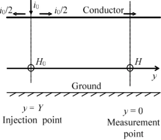
Let us initially consider an infinite single conductor with corona discharge characterized by a uniform excitation function _Γ, i.e. equivalent to the injection of a current i₀_{per unit of length. The current of each elementary section of the}

conductor is divided in two halves, i₀ ₂_{; one moving towards infinite and the}

other towards the point of measurement. This latter half will be calculated in this paper.

We admit that the propagation along the conductor of current i₀ 2_{obeys to}

the same laws as the propagation of a sinusoidal current of the same frequency

0

ω 2π_.

Instead of considering the current, we consider the associated magnetic field H_{. Along a straight line parallel to the conductor, and passing by the point}

of measurement, this field varies like the current itself. Let consider that _H₀ is the field at the injection point of the current i.e. corresponding to the brush discharge location (y=Y , Fig. 1) and H is the field at the point of measurement

(_y₌0_{). In the case of propagation with losses we will have:}

( j) 0e

y

H=H − α + β , (15)

(7)

Fig. 1 – Diagram of a single-phase line.

with:

α - attenuation coefficient in Neper/m. β - constant of wavelength

The real field at the measurement point is the superposition of partial fields due to each elementary section of the conductor; calculated according to next equation:

0 t

H

H =

α

. (16)

Let us consider now the case of a three-phase line and suppose that only conductor (1) produce a corona discharge. We can say that excitation function

1

Γ correspond to a system of currents injected into the three conductors. The propagation of these currents will be studied by decomposing them into three modes and we examine separately the propagation of each one of the obtained modes.

The three modal currents m_i generated by

1

Γ are calculated by the following matrix product:

[ ] [ ]

1 1

1 2

0 3

1 1

0 2 2

0 m

m N C

m

−

Γ

⎧ ⎫ ⎧ ⎫

⎪ ⎪ ₌ ⎪ ⎪

⎨ ⎬ ⎨ ⎬

π ε

⎪ ⎪ ⎪ ⎪

⎩  ⎩ 

, (17)

where

_{[ ]}

N −1

is inverse matrix of the standardized modes and

_{[ ]}

C _{is matrix of}

(8)

With each modal current is associated a modal magnetic field which propagates along the line passing by the point of measurement. By preserving the same notations as for a single-phase line, the field of each mode 'i' relating to injection point at y will be given to the point of measurement (_y₌0_{) by:}

( j )

0e y i

H =H − α + β . (18)

The real elementary field due to the injection of elementary currents in

Y

y= is equal to the sum of the three mode fields:

i

H =

∑

H . (19)

To obtain the total field due to the corona effect along all the conductor, we carry out as in the case of a single-phase line, the quadratic summation of values of all elementary fields by considering the attenuation of the modes; i.e.:

2

2 i

t

i i

H H =

α

∑

. (20)

2.3.2 Formulas for calculation of the fields

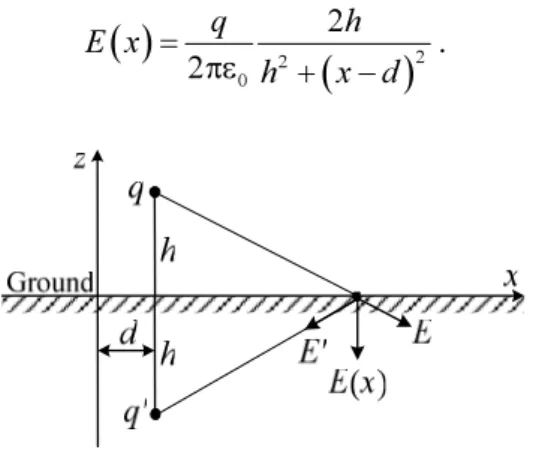
At the ground level, there is only the vertical component of the electric field due to the line charge. To calculate it, we use the method of images. For a charge Q carried by a unit length of the conductor, the field on the ground is given by equation 21 (Fig. 2).

( )

(

)

2

2 0

2 2

q h

E x

h x d

=

πε + −

. (21)

Fig. 2 – Notations for the calculation of the electric field of a conductor above ground-level.

(9)

( )

(

)

2

2 0

2 1

2

i j

j j

E x h q

h x d

= πε

+ −

∑

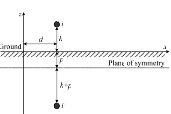
. (22)

We prefer to measure the magnetic component of the guided fields (Fig. 3), it can be given according to the electric component. At the ground level, the horizontal component of the magnetic field due to several conductors 'j'

traversed by current _I_j will be given by:

( )

(

)

2

(

) (

2

)

2

2 1

2 ₂

j j

j j j j

h h p

H x I

h x d h p x d

 ₊ ⎤

⎢ ⎥

= +

⎢ ⎥

π ₊ ₋ ₊ ₊ ₋

⎣ ⎦

∑

. (23)

In the case of propagation without losses, there is a relation of proportionality between the magnetic and the electric components of the guided field:

120

E H = π (24)

Fig. 3 – Notations for the calculation of the magnetic field above the ground.

Until now we considered only one phase with corona effect, but in reality there are excitations of three phases of the line. These excitations are shifted in time and in space; i.e. that each phase generates a disturbance field only throughout formation of the brushes (in the vicinity of the positive peak of the voltage sinusoid).

(10)

It remains now to examine how these fields of phase are considered by the measuring apparatus (CISPR) [9]. The working procedure of the detection system CISPR carries out a particular summation of these fields, according to the following laws established experimentally:

• If one of the three fields is higher than both others of more than 3 dB,

the measuring apparatus takes into account only this one.

• If the difference between two larger fields H1 and H2 is lower than

3 dB, the measuring apparatus indicates a value H calculated by:

(

_CISPR

)

1 2 _1.5dB

2

H =H +H + . (25)

Considering these particular laws, we build the profile of the complete transverse field, as it is measured by CISPR apparatus.

3 Presentation of the Analytical Method

In order to calculate and to plot the level of the disturbance field, we develop a corona effect software (working under MATLAB environment). Calculation is divided into four parts:

Part A_{: Calculation of potential coefficients, matrix of capacities, maximal}

gradients and excitation function for each phase.

Part B:_{Calculation of matrix of wave impedances in order to determine the}

matrix of modes which will be used for the calculation of the modal currents, as well as for the determination of attenuation coefficients.

Part C:_{Calculation of modal currents, modal fields and fields of the phases}

using attenuation coefficients, matrix of modes and useful data of the line.

Part D_{: The real single-phase field is calculated according to the value of}

excitation function for each phase. To obtain the field of the line, the program makes the CISPR summation. Finally the three-phase field is corrected according to the frequency of measurement and the resistivity of ground in the final analysis, to obtain the layout of transverse profile of the disturbance field level.

4 Example of Calculation

We considered a three-phase line with two terns which have next characteristics:

(11)

Apparent power: 600 MVA/tern

Average range: 450m, average Arrow: 3% Height of 1st and 4th phase = 41.8 m

Height of 2nd and 5th phase = 31.8 m Height of 3rd and 6th phase = 22.6 m X-coordinate of 1st and 4th phase = 7.7 m X-coordinate of 2nd and 5th phase = 9.3 m X-coordinate of 3rd and 6th phase = 8.5 m Spacing of under conductors: 40 cm Radius of the conductor = 15.525 mm Number of conductors by beam = 2 Ground wire:

Height: 50 m; X-coordinate: 0m Radius: 9.6 mm

Height of measurement: 2m

5 Presentation of the Results

5.1 220 kV line (under rain)

Fig. 4 represents the modal fields of phase 1 of the first tern.

(12)

Fig. 5 represents the variation of the disturbance field of phases according to the side distance from the line.

-150 -100 -50 0 50 100 150

-5 0 5 10 15 20 25

Transversal distance [m]

Fig. 5 – Variation of real field of phase 1.

Fig. 6 – Variation of Real field of the 220 kV line.

In Fig. 6 we represent the variation of the disturbance field of 220 kV line (the two terns) according to the side distance from the line.

We noted from obtained results that for a 220 kV line, the disturbance field does not reach 32 dB under the axe of the line (42 dB so that the complaint will be admissible.

5.2 400 kV line (under rain)

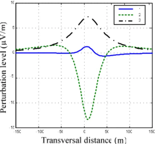
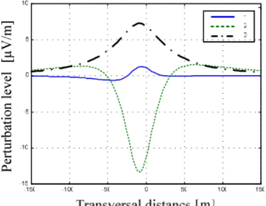
Fig. 7 represents the modal fields of phase 4 of the second tern.

(13)

P

er

tur

ba

ti

o

n l

ev

el

[µ

V

/m

]

Fig. 7 – Modal fields of phase 4 of the 2nd term.

P

er

tur

ba

ti

on l

eve

l [

dB

]

Fig. 8 – Real field of phase 4.

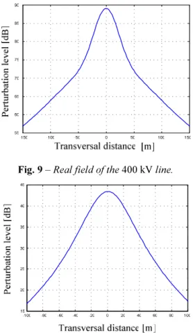
In Fig. 9 is represented the variation of disturbance field of the line (the two terns) for a of 400 kV line according to the side distance to the line.

When the line will be exploited at 400 kV the maximum level is then 89 dB in the middle of the line and is not below 42 dB (value to which the complaint is admissible) only when the distance is more than 200 m.

5.3 Results obtained in dry weather

(14)

Fig. 9 – Real field of the 400 kV line.

Fig. 10 – Disturbance field of the 220 kV line.

(15)

6 Conclusion

Disturbances due to the conductors of high and very high voltage lines depend primarily on the voltage, the section of the conductors and geometry of the pylon. The type of conductor or beam of the line is influent in the form of the profile only by the matrix of the capacities. While passing from a given geometry, from a type of conductor to another, the two matrixes are proportional between them; the profile will not be modified. By comparing the two studied lines, we notice that the disturbing level is more important for the second line than the first because of the maximal gradients which depend on the line voltage. It is necessary, as well from the view point of economic optimization as from the disturbance caused to reception of radio emissions to know the disturbing field generated by a line of transport.

7 References

[1] Claude Gary, Marcel Moreau: The Effect Corona in Alternating Voltage, EYROLLES 1976. [2] Marcel Moreau: Predetermination of the Disturbing Level of the Lines of Transport of

Energy, General Review of Electricity (R.G.E), Tome 80, No. 9 – 1971

[3] Disturbances and Losses of the Lines with 750 kV, According to Two Years of Experimental Installation Operation with VHV, EDF; réf : HM 070-672-CG/MJ (1968).

[4] Dorazio, J.R. Stewart, D.D. Wilson: Six-Phase Power Transmission: First Utility Application, CIGRE Paper 600-01, CIGRE Syposium S 33-91 Compacting Overhead Transmission Lines, Leningradf, 1991.

[5] High Phase Order Transmission Demonstration Research Report EP 88-L3 Phase 3, Empire State Electric Energy Research Corporation, 1997.

[6] Addendum to Interferences Produced by Corona Effect of Electric Systems (Description of Phenomena and Practical Guide of Calculation, CIGRE 1996)

[7] M. Brahami: Impact of the Lines Very High Voltage on the Environment (Limitation of the Level of Consequences) Thesis of Doctorate of State, University of Sidi Bel Abbès Algeria, October 2003.

[8] R.M. Radwan, M.A. Abd.Allah: Electric And Magnetic Fields And Radio Noise From The Extra Towers Crossing The Suez Canal, Reference 36.106 CIGRE 2000