Common Deterministic Shifts
Hans-Martin Krolzig
Department of Economics, and Nuffield College, Oxford.
Juan Toro
European University Institute, Florence
October 30, 2001
Abstract
This paper introduces the concept of common deterministic shifts (CDS). This concept is simple, in-tuitive and relates to the common structure of shifts or policy interventions. We propose a Reduced Rank technique to investigate the presence ofCDS. The proposed testing procedure has standard asymptotics and good small-sample properties. We further link the concept ofCDSto that of super-exogeneity. It is shown thatCDStests can be constructed which allow to test for super-exogeneity. The Monte Carlo evidence indicates that theCDStest for super-exogeneity dominates testing pro-cedures proposed in the literature.
Keywords: Co-breaking, Super-Exogeneity, Reduced Rank Regression, Regime Shifts, Markov Switching.
JEL classification: E32, E37, C32, E24
1 Introduction
Deterministic shifts in the conditional mean of economic variables are a recurrent feature in empirical economics. These shifts happen to affect not just one single economic variable but, contemporaneously, also other related economic variables. Furthermore, some economic time series are affected by several shifts. These shifts might be related linearly and this linear relationship might prevail throughout time. Here we propose a technique that can be used to analyze such phenomena, and can help to gather im-portant information about how breaks are related through economic variables and across time.
Frequently, deterministic shifts are induced by policy changes. Policymakers move the level of some variables in order to affect some target variables and reach specific goals. When deterministic shifts are induced by policymakers, the relationship between common deterministic shifts and super-exogeneity become apparent. Super-exogeneity (see Engle, Hendry and Richard, 1983) establishes conditions un-der which the parameters of the partial model are invariant to changes in the parameters of the marginal model. In an economic context, the marginal model can be thought of as the instrument of the policy-maker (say, the interest rate). The partial model could be thought of as the process for the goal variable (say, the rate of inflation). Super-exogeneity sets conditions under which the partial model has invari-ant parameters, which allows its use for policy analysis despite changes in the marginal model. The
✁
We are grateful to the guest editor, Stephane Gregoir, and two anonymous referees for valuable comments and suggestions on a previous version of this paper. We also thank David Hendry, Soren Johansen, Uwe Hassler and Bent Nielsen for useful comments and discussions. Financial support from the UK Economic and Social Research Council under grant L138251009 is gratefully acknowledged by the first author.
concepts of common deterministic shifts and super-exogeneity are closely related if we limit the set of policymakers interventions to changes in the conditional mean of the marginal process (say, the level of interest rates or the rate of growth of money).
The structure of the paper is as follows: In the next section, we introduce the concept of common deterministic shifts. In
✂✁
we define the model and introduce a reduced rank technique to estimate and test
for common deterministic shifts. The size and power of the proposed technique are investigated in☎✄
with
a Monte Carlo simulation experiment. ✂✆
discusses the concept of super-exogeneity in the framework of common deterministic shifts. In
✞✝
, testing procedures for super-exogeneity are developed which are based on the existence of common deterministic shifts. Their small-sample properties are analyzed in
a small Monte Carlo experiment discussed in ✞✟
. The empirical applicability of the introduced tests is illustrated in
✂✠
, which also comments on their limitations and possible extensions.
✂✡
concludes.
2 The concept of common deterministic shifts
Engle and Kozicki (1993) have recently proposed the idea of common features in time series. This idea is inspired by the concept of cointegration introduced in Granger (1986) and Engle and Granger (1987). Engle and Kozicki (1993) show that a feature is common to a set of time series if a linear combination of them does not have the feature though each of the series individually has it. Some particular examples of this concept are the idea of common cycles, introduced by Engle and Kozicki (1993), and the idea of co-breaking, introduced by Hendry (1997). The concept of co-breaking is closely related to the idea of cointegration: while cointegration removes unit roots from linear combinations of variables, co-breaking can eliminate the effects of regime shifts by taking linear combinations of variables.
Definition 1. Consider☛✌☞✎✍✑✏ to be an✒ dimensional vector process, which is modeled as a vector
autore-gressive (VAR) process of order✓ ,✔✖✕✘✗✚✙✛☞✎✍✢✜✤✣✥✍✧✦✩★✪✍✑✫ Consider a set of✒✭✬✯✮✱✰✳✲ dummy variables✴✵✍✷✶✸
each of which is zero except for unity at times✹✻✺✽✼✾✸, such that✣✥✍✿✜❁❀❃❂
✸❅❄❇❆✾❈ ✸
✴❉✍✷✶✸, or✣✥✍✿✜❋❊❍●■✍, where ❊ is✒✽❏❑✮ and●■✍ is✮▲❏✽▼ with●■✍✿✜◆✕✛✴❉✍✷✶❆▲❖P✴❉✍✷✶◗❘❖❚❙✌❙✌❙❚❖❯✴❉✍✷✶
❂
✙✛❱. The condition for common deterministic
shifts can be written as❲
❱
❊❳✜❃❨❩✫ Thus we have that❬✱✜❋❭☎❪❉❫❵❴❜❛❊❞❝❇✰❡❫ is necessary and sufficient for
❲
❱
✣✥✍✿✜❃❢ for all✹✻✺✽✼ , where❲◆❣✜❃❨ is✒❑❏✩✕✘✒✖❤✩❬❯✙. We say that the equations in the VAR are subject to
common deterministic shifts(CDS)if shifts taking place across the✒ individual equations are linearly
related.
In the definition of common deterministic shifts we just require that shifts be related across variables and through time, which can be expressed as a convenient reduced rank condition in the coefficients of the intervention variables. This concept is different from the co-breaking concept of Hendry (1997) which requires that linear combinations of variables cancel the shifts in the processes. In the following, we
consider the✒ -dimensional linear Gaussian VAR(✓ ):
☞✾✍✿✜
✐
❥
✸❅❄❇❆
✔❦✸❧☞✾✍✷♠❚✸✾✦✳✣✥✍✾✦✳★✪✍✑♥ (1)
where★✪✍♣♦rq✻s✉t✈✕✛❨❩♥✂✇❦✙ and the roots of the vector autoregressive polynomial are within the unit circle,
①
①
①
①②
❤
✐
❀
✸❅❄❇❆ ✔❦✸✛③
✸
①
①
①
①
✜④❢✩✜⑥⑤⑧⑦③✾⑦✽⑨④▼❉✫ Thus there are no unit roots in the system and the possible
non-stationarity is due to the deterministic breaks. This implies that the process possesses the infinite-order vector moving-average representation
☞✾✍✿✜❶⑩
❥
where✔✖✕✘✗✚✙
❸
✕✘✗✚✙ ✜
②
♥ and in the case of a VAR(1) we have that
❸
✸⑥✜❋✔
✸
✫
The methodology proposed in this paper relies on using appropriate shift dummies for known dates. It is assumed that the points at which these shifts occur are known, which avoids the problem of some nuisance parameters. In order to illustrate the reduced rank approach consider a VAR(1) with shifts in the intercept:
☞✾✍✿✜❋✔✱❆❼☞✾✍✷♠❩❆✢✦
❂
❥
✸❅❄❇❆
❈
✸
✴❉✍✷✶✸❚✦✳★✪✍✑✫ (2)
Furthermore, suppose that the shifts are permanent. Then we can use the corresponding shift dummies
to model them: ✴❉✍✷✶✸❇✜ ✕✷✹✻⑨ ✹❺✸❻✙✾♥ where ✕✂✁✵✙ is the indicator function and▼ ✰ ✹ ✸✢✰✳✲ .
CDSis at least of order ✕✘✒✽❤ ❬❯✙ if there exist ✕✛✒✩❤ ❬❯✙ linearly independent vectors✄✥✸ satisfying
✄
❱✸
✣✥✍❇✜☎✄
❱✸
❊❍●■✍✿✜❃❢
such that the✒✳❏ ✕✛✒✩❤ ❬❯✙ matrix❲ ✜ ✕✂✄⑥❆ ❖❹❙✌❙✌❙❹❖✆✄✞✝✠✟ ♠☛✡✌☞ ✙ has rank ✕✛✒✩❤ ❬❯✙ . Then❲
❱
❊ ✜ ❨ so rank
✕✘❊ ✙✱✰ ✒ and the nullity of ❊ determines the order ofCDS. In other words,CDSimplies that❊ is
of reduced rank. Thus,❊ can be decomposed into the product of two matrices,✍ and✎ of full rank❬ ,
such that we can rewrite (2) as:
☞✾✍✿✜❋✔✱❆✑☞✾✍✷♠❩❆✢✦✏✍✑✎
❱
●■✍✎✦✳★✪✍✑✫ (3)
Note that the matrices✍ and✎ are not unique without suitable normalization: if ✒ is any ❬ ❏✳❬
non-singular matrix, then ❊ ✜✓✍✑✎
❱ implies that
✍✔✒✕✒ ♠❩❆
✎
❱
✜✓✍✔✒ ✕✖✎✗✒✕✘ ♠❩❆
✙
❱
✜✓✍ ✎
❱
✜ ❊ as well. If
common deterministic shifts are a property of the data, the coefficient matrix of the dummy regressors will have a reduced rank.
3 Estimating
CDS
vectors by reduced rank regressions
3.1 The reduced-rank regression problem
Maximum likelihood estimation of theCDS✕✘✒ ❤✈❬❯✙☎❤ VAR
✟
✕✓❩✙ is close to the analysis of the likelihood
in cointegrating systems, and both are based in the reduced rank regression technique introduced in An-derson (1951) and Tso (1981). The analogy with the cointegration model is straightforward if one bears
in mind that the regime-dummies ✴✵✍ behave like non-stationary processes if there are structural breaks.
In this case the matrix ❊ determines how the non-stationarity feeds into the variables of the system:
the rank❬ of the matrix❊ gives the number of common deterministic shifts, and theCDSrank (✒✽❤ ❬
or✮▲❤ ❬❯✙ gives the dimension of the space whose one-step predictions are free from these deterministic
breaks. In contrast to the cointegration problem, the number of breaks✮ is not necessarily identical to the
number of endogenous variables in the system, such that the matrix❊ is✒ ❏✖✮ with rank❬❦✬✚✙✜✛❅❫✎✕✘✒✢♥✂✮ ✙❼✫
In matrix notation, we have:
✢
✜✤✣✦✥✳✦ ❊❍● ✦✏✧ ♥ (4)
where✢
❖✜◆✕✷☞⑥❆▲❖✵☞✥◗❦❖❚❙✌❙✌❙❚❖✵☞✩★✢✙ is✒❦❏❹✲ ,✥❃❖✜ ✕✛③ ❆▲❖❯③✧◗❘❖❚❙✌❙✌❙❚❖P③✪★✢✙ is✓✾✒❦❏❹✲ with③ ❱✍
❖✜◆✕✷☞ ❱✍✷♠❩❆
❖❚❙✌❙✌❙❼☞ ❱✍✷♠
✐
✙, ✣ ❖P✜■✕✘✔✱❆▲❖❚❙✌❙✌❙❚❖✵✔
✐
✙ is✒✭❏■✓✾✒ ,✧ ✜◆✕✘★❉❆▲❖❯★ ◗❘❖❵❙✌❙✌❙✾❖✵★✫★ ✙ is✒✭❏✩✲ and● is✮✱❏✩✲ .
❆
✬
Note that, for reasons of simplicity, we assume here that the variables have a zero mean before the first break. If the mean of the variables is non-zero before the first break, an intercept✭ can be added to the model, such that✮
✘
✯✩✰✱✳✲✖✴✵✰✷✶
✘
✯✹✸
✬
✰✻✺✼✺✽✺✾✶
✘
✯✹✸✻✿✪❀
and❁ ✰✫✱❂✲
✭
✰✷❃
✬
✰❄✺✼✺✼✺✻✰✪❃
✿
❀ is ❅❇❆
✲✖✴❉❈❋❊
❅
❊ is✒ ❏ ✮ and of rank ❬ and can be decomposed in two full rank matrices,❊ ✜✤✍✑✎
❱
♥ where✍ are
the loadings and✎ the linear relationships across breaks.
The log-likelihood function for a sample size✲ is easily seen to be
❫✚✗✳✜◆❤ ✒✎✲ ✁ ❫ ✁✄✂ ❤ ✲
✁ ❫ ⑦✇✱⑦ ❤
▼ ✁✆☎ ❭✞✝✕ ✢ ❤ ✣✦✥ ❤ ✍✑✎ ❱● ✙❱✇ ♠❩❆ ✕ ✢
❤ ✣✦✥ ❤ ✍✑✎ ❱● ✙✠✟✿✫ (5)
3.2 Estimation of✣ and✇ conditional on❊
Note that for any fixed✍ and✎ , the maximum of ❫✚✗ is obtained by
✡ ✣▲✕✾✍✑✎ ❱ ✙ ✜◆✕ ✢ ❤ ✍✑✎ ❱ ● ✙✼✥ ❱ ✕✂✥ ✥ ❱ ✙ ♠❩❆ ✫ (6)
If we substitute✣ in (5) by (6), we get
❫✻✗ ✜◆❤ ✒✎✲ ✁ ❫ ✁✄✂ ❤ ✲ ✁
❫ ⑦✇✱⑦ ❤
▼ ✁✆☎ ❭✞✝✕ ✢ ✒❍❤ ✍✑✎ ❱ ● ✒ ✙ ❱ ✇ ♠❩❆ ✕ ✢ ✒❍❤ ✍✑✎ ❱
● ✒ ✙✠✟✿♥ (7)
where✒ ❖✜ ✕
② ★✈❤✏✥ ❱ ✕✂✥ ✥ ❱ ✙ ♠❩❆
✥❜✙ is a✲◆❏✽✲ matrix. Hence, we just have to maximize this expression
with respect to✍ and✇ . For given✍ and✎ , the maximum is obtained for
☛ ✇ ✕✾✍✑✎ ❱ ✙✢✜❡✲ ♠❩❆ ✕ ✢ ❤ ✍✑✎ ❱ ● ✙✂✒ ✕ ✢ ❤ ✍✑✎ ❱ ● ✙ ❱ ✫
Consequently we must maximize:
❤ ✲ ✁ ❫ ① ① ✲ ♠❩❆ ✕ ✢ ❤ ✍✑✎ ❱ ● ✙✂✒ ✕ ✢ ❤ ✍✑✎ ❱ ● ✙ ❱ ① ① (8)
or, equivalently, minimize the determinant with respect to✍ and✎ (see L¨utkepohl, 1991).
3.3 Estimation of✍ conditional on✎
Note that in (7),✢
and● are corrected for✥✚✫ Define the corresponding residuals as:
✕✘✒✭❏✩✲✱✙✌☞✎✍ ❖ ✜
✢
✒✈♥
✕❻✮✱❏✩✲✱✙✌☞✑✏ ❖ ✜❋● ✒✈♥
and the corresponding moment matrices as:
✒ ✸✓❦✜❡✲ ♠❩❆ ☞❘✸✔☞ ❱✓ for ✕✑♥✠✖ ✜ ✢ ♥❼●✈✫
Then (8) can be rewritten as
❤ ✲ ✁ ❫ ① ① ✲ ♠❩❆ ✕✗☞✎✍✯❤ ✍✑✎ ❱ ☞✑✏▲✙☎✕✗☞✎✍❋❤ ✍✑✎ ❱ ☞✑✏▲✙ ❱ ① ① ✫ (9)
For fixed✎ , (8) is maximized with respect to matrix✍ by regression:
☛
✍ ✕✖✎P✙ ✜ ☞✎✍✙✘✾✎ ❱☞✑✏✛✚
3.4 Estimation of✎
Apart from a constant, the concentrated log-likelihood for our reduced rank problem can be shown to be:
❫✚✗
☛
✍ ✕✖✎P✙✾♥✽✎ ♥
☛ ✇ ✘ ☛ ✍❘✕✾✎P✙ ✎ ❱ ✚✂✁ ✜ ❤ ✲ ✁ ❫ ① ① ① ☛ ✇ ✘ ☛
✍ ✕✖✎P✙ ✎
❱ ✚ ① ① ① ✜ ❤ ✲ ✁ ❫ ① ① ① ① ▼ ✲ ✕✗☞✎✍✯❤ ☞✎✍✞☞ ❱✏ ✎ ✝✎ ❱ ✕✗☞✑✏✢☞ ❱✏ ✙ ✎ ✟ ♠❩❆ ✎ ❱ ☞✑✏▲✙☎✕✗☞☎✄✱❤ ☞✎✍✞☞ ❱✏ ✎ ✝✎ ❱ ✕✗☞✑✏✛☞ ❱✏ ✙✎ ✟ ♠❩❆ ✎ ❱ ☞✑✏▲✙ ❱ ① ① ① ① ✜ ❤ ✲ ✁ ❫ ① ① ① ① ▼ ✲ ☞✎✍✖✕ ② ❤ ☞ ❱✏ ✎ ✝✎ ❱ ✕✗☞✑✏✢☞ ❱✏ ✙✎ ✟ ♠❩❆ ✎ ❱ ☞✑✏▲✙☎✕ ② ❤ ☞ ❱✏ ✎ ✝✎ ❱ ✕✗☞✑✏✢☞ ❱✏ ✙ ✎ ✟ ♠❩❆ ✎ ❱ ☞✑✏▲✙ ❱ ☞ ❱✍ ① ① ① ① ✜ ❤ ✲ ✁ ❫ ① ① ① ① ▼ ✲ ☞✎✍✝✆ ② ❤ ✘✾✎ ❱ ☞✑✏✛✚ ❱✟✞ ✕✖✎ ❱ ☞✑✏▲✙ ✘✾✎ ❱ ☞✑✏ ✚ ❱✠ ♠❩❆ ✕✖✎ ❱ ☞✑✏▲✙☛✡ ☞ ❱✍ ① ① ① ① ✜ ❤ ✲ ✁ ❫ ① ① ✒ ✍✢✍✯❤ ✒ ✍✛✏ ✎❵✕✖✎ ❱ ✒ ✏✣✏ ✎P✙ ♠❩❆ ✎ ❱ ✒ ✏ ✍ ① ① ✫ (11)
By using the identity
① ① ① ① ① ✒ ✍✢✍ ✒ ✍✛✏ ✎ ✎ ❱ ✒ ✏ ✍ ✎ ❱ ✒ ✏✣✏ ✎ ① ① ① ① ① ✜ ① ① ✎ ❱ ✒ ✏✣✏ ✎ ① ① ① ① ✒ ✍✢✍❡❤ ✒ ✍✛✏ ✎❵✕✖✎ ❱ ✒ ✏✣✏ ✎P✙ ♠❩❆ ✎ ❱ ✒ ✏ ✍ ① ① ✜ ⑦ ✒ ✍✢✍■⑦ ① ① ✎ ❱ ✒ ✏✣✏ ✎❜❤ ✎ ❱ ✒ ✏ ✍ ✒ ♠❩❆ ✍✢✍ ✒ ✍✛✏ ✎ ① ① ♥
Equation (11) can be expressed as:
❫✚✗
☛
✍ ✕✖✎P✙✾♥✽✎ ♥
☛ ✇ ✘ ☛ ✍❘✕✾✎P✙ ✎ ❱ ✚☞✁ ✜ ❤ ✲ ✁ ❫ ⑦ ✒ ✍✢✍■⑦ ① ① ✎ ❱ ✒ ✏✣✏ ✎✱❤ ✎ ❱ ✒ ✏ ✍ ✒ ♠❩❆ ✍✢✍ ✒ ✍✛✏ ✎ ① ① ⑦✎ ❱ ✒ ✏✣✏ ✎✾⑦ ✜ ❤ ✲ ✁ ❫ ⑦ ✒ ✍✢✍■⑦ ① ① ✎ ❱ ✘ ✒ ✏✣✏✤❤ ✒ ✏ ✍ ✒ ♠❩❆ ✍✢✍ ✒ ✍✛✏✛✚✞✎ ① ① ⑦✎ ❱ ✒ ✏✣✏ ✎✾⑦ ✫
Hence, the maximum of ❫✚✗ is given by
✙✜✛❅❫ ✌ ① ① ✎ ❱ ✘ ✒ ✏✣✏ ❤ ✒ ✏ ✍ ✒ ♠❩❆ ✍✢✍ ✒ ✍✛✏✢✚ ✎ ① ① ⑦✎ ❱ ✒ ✏✣✏ ✎✾⑦
and following a basic theorem of matrix analysis (see, for example, Johansen, 1995, Lemma A.8), this
factor is minimized among all✒ ❏ ❬ matrices✎ by solving the eigenvalue problem
① ①✍ ✒ ✏✣✏✤❤ ✘ ✒ ✏✣✏ ❤ ✒ ✏ ✍ ✒ ♠❩❆ ✍✢✍ ✒ ✍✛✏ ✚ ① ① ✜❃❢
or, for✎✩✜ ▼▲❤
✍
♥ the eigenvalue problem
① ① ✎ ✒ ✏✣✏♣♠ ✒ ✏ ✍ ✒ ♠❩❆ ✍✢✍ ✒ ✍✛✏ ① ① ✜❃❢
for eigenvalues✎❚✸ and eigenvectors✏ ✸❺♥ such that
✎❵✸ ✒ ✏✣✏✑✏ ✸⑥✜ ✒ ✏ ✍ ✒ ♠❩❆ ✍✢✍ ✒
✍✛✏✑✏ ✸❺✫ (12)
If we normalize✎ such that✎
❱
✒
✏✣✏ ✎ ✜
②
✡ then the vectors of
☛
✎ are given by the eigenvectors
corres-ponding to the❬ largest eigenvalues of
✒ ✏✣✏✤❤ ✒ ✏ ✍ ✒ ♠❩❆ ✍✢✍ ✒
✍✛✏ . The maximum log-likelihood under the
rank✕✘❊ ✙♣✜❋❬ restriction is given by:
✙ ❪✓✒ ❫✚✗✳✜◆❤ ✒✎✲ ✁ ❫ ✁✄✂ ❤ ✲
✁✕✔ ❫ ⑦
✒ ✍✢✍■⑦✪✦ ✡ ❥ ✸❅❄❇❆ ❫ ▼❦❤✗✖✎❵✸✘✁✚✙ ❤ ✒✎✲
✁ ♥ (13)
since, by choice of
☛
✎ , we have that✎
❱
✒
✏✣✏ ✎ ✜
②
✡ ♥ as well as✎
❱ ✒ ✏ ✍ ✒ ♠❩❆ ✍✢✍ ✒
3.5 Testing for theCDSrank
SinceCDS(✒✽❤✤❬ ) impliesCDS(✒✽❤✤❬❜❤ ▼ ), it seems natural to seek the maximum degree ofCDS. In
general, two cases have to be distinguished. In the first case , the number of potential breaks✮ is less than
the dimension of the system✒✢♥ ✜ ✙✜✛❅❫✥✕❻✮❉♥❼✒✿✙▲✜ ✮❑✰ ✒✢✫ In the second case, the number of potential
breaks ✮ is not less than the dimension of the system✒ , i.e. ✜✤✙✜✛❅❫✥✕❻✮❉♥❼✒✿✙✢✜❋✒✭✬✯✮❉✫
Suppose in the following that✒✭✬✯✮❉✫ Then the following hypotheses might be of interest:
(i) CDS(✒ ) : ❭☎❪❉❫❵❴✾✕✘❊ ✙ ✜❃❢ . No breaks.
(ii) CDS(✒✩❤ ❬ ):❭☎❪❉❫❵❴✎✕✘❊ ✙ ✜❋❬ ,❢ ✰ ❬■✰ ✒ . There are breaks which are common to the processes.
(iii) CDS(❢ ):❭☎❪❉❫❵❴✎✕✘❊ ✙ ✜❋✒ . There are as many linearly independent breaks as variables in the system.
Following Anderson (1951), the likelihood ratio test statistic for testing the CDS✕✘❬❯✙ against the
CDS✕✘✒✿✙ is given by:
❤
✁
❫
✁
✕ ✒ ✕✘❬❯✙✻⑦ ✒ ✕✘✒✿✙✑✙ ✜◆❤✻✲
✟
❥
✸❅❄❉✡✄✂❇❆
❫ ▼❦❤✗✖✎❵✸✘✁■♥
which has a☎
◗
-distribution with degrees of freedom equal to (✒✽❤ ❬❯✙☎✕❻✮▲❤ ❬❯✙.
4 Some Monte Carlo results
4.1 Design of the Monte Carlo
In this section we analyze the size and power of the rank test for common deterministic shifts. The data
generation process (DGP) is a two-dimensional process☞✥✍✿✜◆✕✝✆ ✍ ❖P③✌✍❺✙
❱ where
③✌✍ does not feedback into
the first equation and there are two breaks in the intercept term at time✹✌❆ and✹✑◗ ,
✞
✆ ✍ ③✌✍✠✟
✜
✞
❢P✫ ✟❉✝
❢P✫
✝
❢ ✡☛✟
✞
✆ ✍✷♠❩❆ ③✌✍✷♠❩❆☞✟
✦✳❊
✞
✴❉✍
✬
✴❉✍✍✌☞✟
✦
✞
★❉❆✛✍ ★ ◗❺✍✎✟
(14)
where
✞
★❉❆✛✍ ★ ◗❺✍✎✟
♦◆q✻s✉t ✞✏✞
❢
❢✑✟
♥
✞
▼❶❢ ❢ ▼✒✟✏✟
✫
The matrix of intervention coefficients❊ embeds information about the size of the shifts, and the
rela-tionship of the shifts across variables and time. The interpretation of the model will critically depend on
the assumed rank of the matrix❊ :
(i) ❭☎❪❉❫❵❴✎✕✘❊ ✙ ✜❃❢ . No breaks.
(ii) ❭☎❪❉❫❵❴✎✕✘❊ ✙ ✜ ▼ . There are breaks which are common to both processes.
(iii) ❭☎❪❉❫❵❴✎✕✘❊ ✙ ✜
✁
(full rank). There are breaks independent to each process.
We consider two specifications for ❊ . In the first specification,❊ is of full rank:
❊ ❆ ✜✔✓
✞
▼ ✫
✝
✫
✝
▼✕✟
✫
The second specification for❊ , denoted❊ ◗ , has reduced rank:
❊ ◗▲✜✔✓
✞
▼
✖
▼
✂
✁
This corresponds to the case ofCDS, where ✖
defines the relationship of the breaks across equations,
✂
defines the relationship of breaks across time and ✓ defines the magnitude of the breaks measured in
terms of the standard deviation. In the Monte Carlo experiment, we analyze the properties of theCDS
test when we allow ✖
, ✂
and ✓ to vary. We will consider the following values:
✖
✺ ☛✧❢P✫
✁
✝
♥☎❢P✫
✝
♥✌▼❉✏ ,
✂
✺✭☛✧❢P✫
✁
✝
♥☎❢P✫
✝
♥✌▼❉✏ and✓❑✺✭☛❉▼❉♥✌▼❉✫
✝
♥
✁
✏ .
The benchmark case will have ✡✭✜❁❢P✫
✠
, but one might be interested in analyzing the size of the test
when the process for③✪✍ becomes close to the unit root. That is,✡✯✺ ☛✧❢P✫
✡✵✝ ♥☎❢P✫
✡✵✟❉✝ ♥☎❢P✫
✡❉✡
✏ . Furthermore,
in order to study how the distance between breaks affects theCDStest, we consider different distances
between the breaks. As the break points are defined as fractions of the sample size,✹✌❆▲✜ ❆ ✲ and✹✑◗❘✜
◗❼✲ , we will parametrically vary the first break point, ❆ ✺ ☛✧❢P✫
✁
❢P♥☎❢P✫
✁
▼❉♥✌✫✌✫✌✫❹♥☎❢P✫
✆
✏ , while keeping the
second break point fixed, ◗▲✜❃❢P✫
✟
.
We consider three different sample sizes: ✲❃✜
✝
❢P♥✌▼✧❢❉❢ and▼
✝
❢ . The number of replications is
✁
✜
▼✧❢❉❢❉❢❉❢ . If we had relied on a full factorial design, the number of experiments would have been 18225. We
therefore focus on two benchmarkDGPs in our Monte Carlo study: t✄✂✆☎❇❆ is characterized by✕✘❊ ❆✞✝ ✓ ✜
✁
✝ ✡ ✜ ❢P✫
✠
✝ ❆ ✜ ❢P✫
✁
♥ ◗✱✜ ❢P✫
✟
✙ and will be used to study the power properties of theCDStest. t✄✂✆☎⑥◗
is defined by ✕✘❊ ◗✟✝
✖
✜ ▼❉♥
✂
✜ ▼❉♥ ✓ ✜
✁
✝ ✡ ✜❃❢P✫
✠
✝ ❆✚✜❃❢P✫
✁
♥ ◗❦✜❃❢P✫
✟
✙ and allows to investigate the size
properties of theCDStest given the reduced rank of its matrix of intervention coefficients.
4.2 Evaluation of the Monte Carlo
Table 1 presents the rejection frequencies of theCDStest for our simulated t✄✂✆☎⑥◗ for nominal sizes
from▼✟✠ to
✁
❢✡✠ . It can be seen that the real size differs from the nominal size and this difference cannot
be explained by Monte Carlo sampling variation. Table 2 presents the rejection frequencies for the test
statistic ✒ ❷✭❖ ❭☎❪❉❫❵❴✾✕✘❊ ✙ ✜ ▼ against ✒✩❆ ❖ ❭☎❪❉❫❵❴✎✕✘❊ ✙ ✜
✁
when the model simulated is t✄✂✆☎⑥❆ . This
delivers the power of theCDStest for our benchmark case.
Table 1 Size of theCDSrank test.
T 20% 10% 5% 1%
50 0.243 0.133 0.068 0.015
100 0.231 0.123 0.064 0.016
150 0.222 0.117 0.062 0.012
Note: Rejection frequencies for the test statistic ☛✆☞
✰✍✌✏✎✒✑✟✓✗✲✕✔✤❀☛✱✕✴ against
☛
✬
✰✍✌✏✎✒✑✟✓ ✲✕✔✤❀ ✱✗✖
for the benchmark✘✚✙✜✛ ✌ .
Table 2 Power of theCDSrank test.
T 20% 10% 5% 1%
50 0.954 0.909 0.810 0.673
100 0.996 0.989 0.949 0.924
150 0.999 0.998 0.985 0.978
Note: Rejection frequencies for the test statistic ☛✆☞
✰✍✌✏✎✒✑✟✓✗✲✕✔✤❀☛✱✕✴ against
☛
✬
✰✍✌✏✎✒✑✟✓ ✲✕✔✤❀ ✱✗✖
for the benchmark✘✚✙✜✛
✬
.
Figure 1 compares the theoretical and empirical quantiles of theCDStest statistic for the reduced
rank of❊ : ✒ ❷ ❖❩❭☎❪❉❫❵❴✾✕✘❊ ✙ ✜ ▼ against✒✩❆■❖❩❭☎❪❉❫❵❴✾✕✘❊ ✙ ✜
✁
. The simulated model is the benchmark
t✄✂✆☎✎◗ and the sample sizes are✲❃✜
✝
❢P♥✌▼✧❢❉❢ and▼
✝
a☎
◗
with one degree of freedom. The results indicate that the empirical size is slightly higher than the nominal size, but the simulated quantiles approach the theoretical quantiles of the asymptotic distribution
with increasing sample size relatively fast for✲
✝
❢P✫
0 5 10 15
5 10 15
QQ plot for T = 50
0 5 10 15
5 10 15
QQ plot for T = 100
0 5 10 15
5 10 15
QQ plot for T = 150
Figure 1 QQ plot of theCDStest for the reduced rank of❊ .
In order to compare the power of theCDStest against its true size we will make use of size-power
curves. We thus construct two different experiments: in the first experiment theDGPsatisfies the null of
common deterministic shifts, and in the second experiment the matrix of interventions coefficients has full rank.
Let us denote the test statistic in replication ✖ by✁ ✓ ✫ With✁ ✓ there is an associated✓ value (✓ ✓ ✜
✓❇✕✂✁ ✓ ✙), obtained from our asymptotic distribution, which is☎
◗
✕ ▼ ✙ . For any point☞✾✸ in the ✕✛❢P♥✌▼ ✙ interval
we can define the empirical distribution function (EDF) of✓ ✓ as:
✄
✕✷☞✾✸❻✙ ✜
▼
✁
☎
❥
✓✂❄❇❆
✕✓ ✓✱✰ ☞✾✸❺✙❼✫
The EDF
✄
✕✷☞✾✸❻✙ reports the probability of getting a✓ value less than☞✥✸ under the null. Following the
sug-gestion of Davidson and MacKinnon (1997) the EDF is evaluated at ✜
✁
▼
✝
points☞✥✸ ♥ ✕✿✜ ▼❉♥✌✫✌✫✌✫✿♥ ♥
where ✜
✁
▼
✝
and☞✾✸✢✺✭☛✧❢P♥☎❢P✫❢❉❢P▼❉♥☎❢P✫❢❉❢
✁
♥✌✫✪✫✌✫❹♥☎❢P✫ ✡❉✡❉✡
✏ . We can then obtain a✓ -value plot plotting
✄
✕✷☞✎✸❺✙
against☞✾✸❺✫ If the test is well-behaved (i.e. the test is rejected just about the right proportion of times) the
plot should be close to the 45 degree line.
If we denote by✄
✕✷☞✾✸❻✙ the EDF under the alternative, and the same random numbers are used when
simulating the errors under the null and the alternative, then the size-power curve is obtained plotting
✄
✕✷☞✾✸❻✙ against
✄
✕✷☞✾✸❻✙.
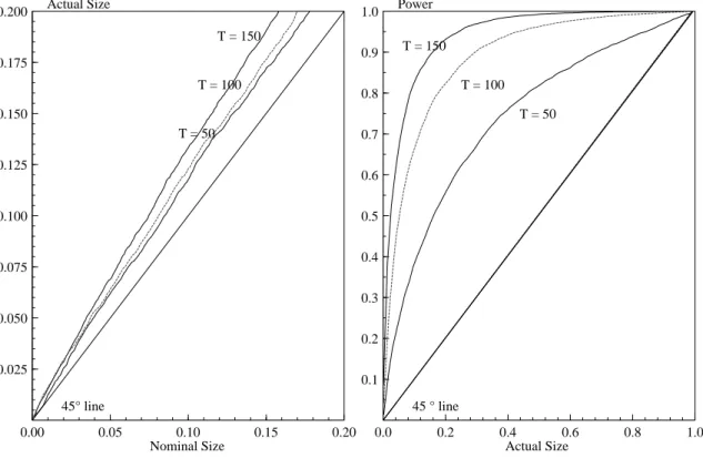
The✓ -value plots in Figure 2 help to summarize and complement the information contained in Tables
0.00 0.05 0.10 0.15 0.20 0.025
0.050 0.075 0.100 0.125 0.150 0.175
0.200 Actual Size
Nominal Size T = 50
T = 100 T = 150
45° line
0.0 0.2 0.4 0.6 0.8 1.0
0.1 0.2 0.3 0.4 0.5 0.6 0.7 0.8 0.9 1.0
Actual Size Power
T = 50 T = 100 T = 150
45 ° line
Figure 2 Size-power curve analysis.
against✒✩❆▲❖✵❭☎❪❉❫❵❴✎✕✘❊ ✙ ✜
✁
is plotted which is based on the empirical distribution of the✓ -values of our
test statistic when the simulatedDGPis the benchmark t✄✂✆☎⑥◗ . We can see that theCDStest tends to
overreject slightly. This overrejection tends to decrease quickly as the sample size increases with the
✓ -value plot approaching the 45 degree line. The plot is truncated for values of☞❩✸▲⑨◆❢P✫
✁
since relative small test sizes are of interest. The right panel of Figure 2 depicts the corresponding power-size curve.
The power always exceeds hugely the actual size and is excellent for✲❃✜ ▼✧❢❉❢ and▼
✝
❢ .
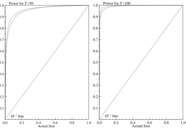
The robustness of the previous results is analyzed in Figure 3, which presents evidence of the
size-power trade-off under parametric variations of the benchmark t✄✂✆☎⑥◗ . Each plot contains the size-power
curve (bold line) for the CDStest statistic for the presence of one common deterministic shift, ✒✽❷ ❖
❭☎❪❉❫❵❴✎✕✘❊ ✙♣✜ ▼ against✒✩❆❘❖ ❭☎❪❉❫❵❴✎✕✘❊ ✙♣✜
✁
for three sample sizes✲ ✜
✝
❢P♥✌▼✧❢❉❢ and▼
✝
❢P✫ For each
para-meterization of theDGP, the size-power curve is compared with the size-power curve in the benchmark
t✄✂✆☎✎◗ (thin line).
Plots [A] and [B] compare the size-power curves in the benchmark t✄✂✆☎❩◗ with✓ ✜r▼❉✫
✝
and✓✽✜ ▼
respectively. Plot [C] compares the size-power curves in the benchmark t✄✂✆☎⑥◗ with that obtained when
✖
✜ ❢P✫
✝
✫ Plot [D] visualizes the effects of
✂
✜ ❢P✫
✝
✫ Finally, Plot [E] graphs the size-power curve
ob-tained when✓ ✜ ▼ and
✖
✜
✂
✜❃❢P✫
✝
✫ From the plots, we can see that the power for a given size remains
largely unchanged with different parameterization of the benchmarkDGP. There is, however, a
substan-tial reduction in power relative to our benchmark t✄✂✆☎❩◗ when the size of the breaks is lowered as in the
case of✓ ✜ ▼ and
✖
✜
✂
✜❃❢P✫
✝
.
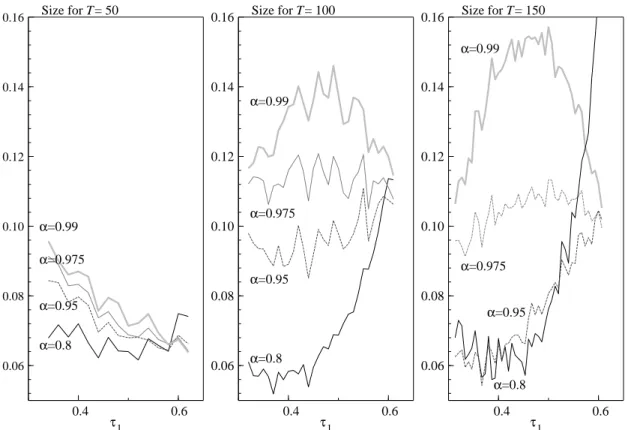
We next analyze how the position of the breaks may affect the size and the power of the CDS
test by changing the point of occurrence of the first break, allowing ❆ to vary from ❢P✫
✁
to ❢P✫
✆
of the
sample ( ❆ ✺④☛✧❢P✫
✁
❢P♥☎❢P✫
✁
▼❉♥✌✫✌✫✌✫❹♥☎❢P✫
✆
✏ ). The second breaks is always fixed at ✹❼◗ ✜ ◗❼✲ for ◗ ✜
❢P✫
✟
0.0 0.1 0.2 0.1
0.2 0.3 0.4 0.5 0.6 0.7 0.8 0.9 1.0
Actual Size [A] Power for k=1.5
T= 50 T= 100 T= 150
45 ° line
0.0 0.1 0.2
0.1 0.2 0.3 0.4 0.5 0.6 0.7 0.8 0.9 1.0
Actual Size [B] Power for k=1
T= 50 T= 100 T= 150
45 ° line
0.0 0.1 0.2
0.1 0.2 0.3 0.4 0.5 0.6 0.7 0.8 0.9 1.0
[C] Power for ϕ= .5
T= 50 T= 100 T= 150
45 ° line
Actual Size 0.0 0.1 0.2
0.1 0.2 0.3 0.4 0.5 0.6 0.7 0.8 0.9 1.0
[D] Power for π=.5
T= 50 T= 100 T= 150
45 ° line
Actual Size 0.0 0.1 0.2
0.1 0.2 0.3 0.4 0.5 0.6 0.7 0.8 0.9 1.0
T= 100 T= 150
45 ° line [E] k=1,ϕ=π=.5
Actual Size
Figure 3 Size-power curve analysis for theCDSrank test.
✡ ✺ ☛✧❢P✫
✠
♥☎❢P✫ ✡✵✝
♥☎❢P✫ ✡✵✟❉✝
♥☎❢ ✫ ✡❉✡
✏ , which allows the investigation of the behavior of the test as the process
for ③✌✍ gets closer to a unit root process. As in the previous experiments, three different sample sizes
(✲❃✜
✝
❢P♥✌▼✧❢❉❢ and▼
✝
❢ ) are considered.
The Monte Carlo results shown in Figures 4 and 5 depict the size and power of theCDStest for a
given nominal size of
✝
✠ . In these plots the vertical axis measures the size and the power, respectively,
and the horizontal axis measures the location of the first break as a fraction of the sample size. When interpreting the plots, the reader should be aware that Figure 5 depicts the power for the given nominal
size. From the graphs one can see that the actual size clearly deviates from the nominal size when✡ gets
closer to unity. Furthermore, for ✡❡✜ ✫
✠
the actual size increases rapidly as the break points get closer
to the second break point. For✲ ✜
✝
❢ power increases with greater distance from the second break.
The power is uniformly strong for✲ ▼✧❢❉❢ . Overall, the Monte Carlo results are very promising. The
asymptotic☎
◗
distribution of theCDStest is found to provide a good approximation of the small-sample
0.06 0.08 0.10 0.12 0.14 0.16
α=0.8
α=0.95
α=0.975
α=0.99 Size for T= 50
τ1
0.4 0.6
0.06 0.08 0.10 0.12 0.14 0.16
α=0.99
α=0.975
α=0.95
α=0.8
Size for T= 100
τ1
0.4 0.6
0.06 0.08 0.10 0.12 0.14 0.16
α=0.99
α=0.975
α=0.95
α=0.8 Size for T= 150
τ1
0.4 0.6
Figure 4 Size of the test statistic for different values of✡ and ❆ varying from❢P✫
✁
to❢P✫
✆
.
0.80 0.85 0.90 0.95 1.00
α=0.8
α=0.95
α=0.975
α=0.99 Power for T= 50
τ1
0.4 0.6
0.80 0.85 0.90 0.95 1.00
α=0.99
α=0.975
α=0.95
α=0.8 Power for T= 100
τ1
0.4 0.6
0.80 0.85 0.90 0.95
1.00 Power for T= 150
τ1
0.4 0.6
Figure 5 Power of the test statistic for different values of✡ and ❆ varying from❢P✫
✁
to❢P✫
✆
5 Super-exogeneity in the Presence of Common Deterministic Shifts
The previous section used reduced rank regressions as a modelling device for finding common determ-inistic shift features. In this section we present an alternative analysis. Though the concept of common deterministic shifts has been introduced in terms of an unrestricted model, its most insightful application involves conditional models.
5.1 The concept of super-exogeneity
Before we discuss how common deterministic shifts in the conditional mean are related to the concept of super-exogeneity, let us introduce the definitions of weak and super-exogeneity. We will consider a
statistical model for the vector process☞✥✍✱✜ ✕✝✆
❱✍ ❖❯③
❱✍
✙
❱ with parameters
✺✂✁ . We are interested in a
function of , called the parameters of interest, i.e. ✁ ✜ ✁✢✕ ✙❼✫
Definition 2. Weak exogeneity: The process③✧✍ is called weakly exogenous for the parameter of interest
✁ if there exist a parameterization of the model such that:
✄
✕✷☞⑥❆✌♥✌✫✉✫✉♥✑☞✩★ ✝ ✡❹♥✆☎✿✙♣✜
★
✝
✍❄❇❆✟✞
✍❼✕✝✆ ✍☎⑦③✌✍❼♥✑☞⑥❆✌♥✌✫✉✫✉♥✑☞✾✍✷♠❩❆ ✝✆☎✿✙✡✠ ✍☎✕✛③✌✍✞⑦☞⑥❆✌♥✌✫✉✫✉♥✑☞✾✍✷♠❩❆ ✝ ✡ ✙❼♥
where ✕✡❹♥✆☎✿✙✻✺ ✔ ❏☞☛ and✁ ✜ ✁✢✕✌☎✿✙ is identified.
In order to define super-exogeneity we need to define the class of interventions affecting theDGP.
We define the class of interventions under consideration, as any action ✎✾✍❑✺✎✍♣✍ by an agent from his
available action set✍ ✍, which alters from its current value to a different value ✍✿✜
✞
✕ ✎❵✍✑♥ ✙❼✫ The class
of interventions◗
✍ can then be formally defined as:
✍ ✜ ☛ ✎❵✍❹❖ ✍✿✜
✞
✕ ✎❵✍✑♥ ✙❼♥ ✎❵✍❹✺✏✍♣✍ ✏❉✫
Definition 3. Super-exogeneity: The process ③✧✍ is called super exogenous for the parameter of interest
✁✢✕✌☎✿✙ and the class✍ of interventions if there exists a parameterization of the model such that:
✄
✕✷☞⑥❆✌♥✌✫✉✫✉♥✑☞✩★ ✝ ✡ ❆✪♥✌✫✉✫✉✫✉♥ ✡ ★♣♥✆☎✿✙ ✜
★
✝
✍❄❇❆✟✞
✍❼✕✝✆ ✍☎⑦③✌✍✑♥✑☞⑥❆✪♥✌✫✉✫✉♥✑☞✾✍✷♠❩❆ ✝✆☎✿✙✡✠ ✍☎✕✛③✌✍✂⑦☞⑥❆✪♥✌✫✉✫✉♥✑☞✾✍✷♠❩❆ ✝ ✡⑥✍ ✙❼♥
where ✕✡ ❆✪♥✌✫✉✫✉✫✉♥ ✡ ★♣♥✆☎✿✙ ✺✏✍✯❏☞☛ and✁ ✜ ✁✢✕✌☎✿✙ is identified.
Super-exogeneity establishes conditions under which the Lucas critique can be refuted. Consider ✆❯✍
as the variable about which agents form plans given all information✑❇✍✷♠❩❆ available at time✹✚❤ ▼ . We
would be interested in analyzing the invariance of☎ when the marginal process changes. Favero and
Hendry (1992) distinguishes two levels of the critique applicable to☎ .
Level A: At this level of the critique, ☎ may change due to changes in economic policy control rules.
Level B : At this level of the critique, ☎ might vary because of changes in economic environment that
alter expectations.
At level A, changes in the distribution of variables that are under the control of a policymaker lead to variations in the parameters of empirical models. In this case future expectations are not necessarily involved. A case of this critique is the Lucas (1975) supply function. The level B of the critique cor-responds to the use of backward-looking econometric specifications when agents use forward-looking specifications.
✌
5.2 The model
Consider the VAR(✓ ) in Equation (1). If we apply the partition☞✥✍✿✜◆✕✝✆
❱✍ ❖❯③
❱✍
✙
❱ and consider just one lag,
✓✩✜ ▼ , we have:
✞
✆ ✍ ③✌✍✠✟
✜
✞
✔✱❆✑❆ ✔✱❆❺◗ ✔ ◗☎❆ ✔ ◗✑◗☞✟
✞
✆ ✍✷♠❩❆ ③✌✍✷♠❩❆ ✟
✦
✞
✣ ✍ ✣✂✁ ✍✠✟
✦
✞
★ ✶✍ ★✄✁✂✶✍✠✟
✫ (15)
If we consider all information as of time✹ ❤ ▼ and denote it by✑❇✍✷♠❩❆ , the unrestricted model can be
written as:
✞
✆ ✍ ③✌✍
①
①
①
①
①
✑❩✍✷♠❩❆
✟
♦✖q✻s✉t ✞✏✞
✣
☎
✶✍
✣
☎
✁✂✶✍
✟
♥
✞
✇
✆ ✇ ✁ ✇✝✁ ✇✝✁✞✁ ✟✏✟
♥ (16)
where✣
☎
✶✍
❖✜✤✧❡✕✝✆ ✍ ⑦✆✑❩✍✷♠❩❆✌✙,✣
☎
✁✂✶✍
❖✜✤✧❡✕✛③✌✍✻⑦✆✑❩✍✷♠❩❆✞✙ and the intercept ✣❩✍ is subject to regime shifts.
Hendry and Mizon (1998) have advanced two different situations in which common deterministic shifts could play an essential role in modelling. They refer to these situations as the contemporaneous
correlation case and the behavioral relation case. The contemporaneous and behavioral cases can be
identified with the level A and level B of the Lucas critique presented above. In the contemporaneous
correlation case✆❉✍ can be seen as a policy variable whereas③✪✍ is an instrument that policymakers can
use in order to reach their goal in terms of✆✵✍ . The behavioral relation case refers to the situation in
which agents form rational expectations (about③✧✍) and there is an interest in analyzing how changes in
the expectations may affect the plan of the agents (✆✵✍).
✟
In both cases, common deterministic shifts are introduced to justify invariance of the conditional model due to changes in the marginal model. The
ex-istence of a specific linear relationship relating breaks (✇ ✁✪✇
♠❩❆
✁✞✁ ) under the presence of weak exogeneity
(see Engle et al., 1983) define necessary conditions for a valid policy analysis.
In order to illustrate the empirical importance of the Lucas critique and the empirical applicability of the super-exogeneity test that we will propose later, we will briefly discuss an economic example of the level A of the critique. We mentioned above that a case of level A of the critique is the Lucas supply function. In the model presented in Lucas (1975) and discussed in Lucas (1976), the economy is con-sidered as formed by suppliers of goods distributed over
✁
distinct markets✕✢✜ ▼❉♥✌✫✌✫✌✫❇♥
✁
. The quantity supplied in each market is composed of two components:
✆ ✸✍❇✜ ✆
✐
✸✍ ✦ ✆
☎
✸✍
♥
where✆
✐
✸✍and
✆
☎
✸✍ are respectively the permanent and transitory components of output supplied by
indi-vidual✕ to the market. Transitory supply varies with the relative prices of good in market✕:
✆
☎
✸✍
✜ ☎ ✕✓❚✸✍⑥❤✽✓
✠
✸✍
✙❼♥ (17)
where✓❚✸✍ and✓
✠
✸✍ are the local and general level of prices in the economy. The local level of prices in
market✕✢✕✓❚✸✍ ✙ consist of two components:
✓❚✸✍✿✜✤✓❚✍✎✦ ③✌✸✍✑✫
✡
Many models in economics are expressed in terms of rational expectations. They can be expressed as the behavioral rela-tion:
☛
✲✌☞ ✯✎✍✑✏✑✯✹✸ ✬
❀☛✱✓✒
✁
✔
❈✖✕
☛
✲
✮
✯✎✍✑✏✑✯✹✸ ✬
❀
or in short form:✒ ✔✆✗
✯
✱✓✒
✁
✔
❈✘✕✙✒✛✚
✗
✯
, where✒ ✔✆✗
✯
are the agent’s plan about variables they control and✒✜✚
✗
✯
Suppliers do not observe these components separately and just observe✓✎✸✍. Conditioned on all
informa-tion prior to time✹ (✑⑥✍✷♠❩❆ ),✓❚✍ is assumed to be normally distributed with mean✓
✍ and variance
◗
:
✓❚✍❇♦◆q✻s✉t❦✕✓
✍
♥
◗
✙❼✫
The component③✌✸✍ is independent across time and across markets and is distributed normally with mean
0 and variance ◗
:
③✌✸✍✿♦◆q✻s✉t❦✕✛❢P♥
◗
✙❼✫
The general price is an average over all markets and considering a law of large number for③ ✸✍, the general
price level is given by✓✾✍✑✫ The estimate of the conditional mean of✓✾✍ is✓
✠
✸✍ and can be obtained as:
✓
✠
✸✍
✜
✁
❛✓❚✍✂⑦✑❩✍✷♠❩❆✌♥✘✓❚✸✍✘❝✎✜◆✕▼❦❤ ✙❅✓❚✸✍✎✦ ✓ ✍ with
✜
◗
◗
✦
◗
✫ (18)
Substituting expression for✓
✠
✸✍ in (17), averaging over all markets and adding up the permanent
compon-ent we have the Lucas supply function:
✆ ✍✿✜ ☎ ✕✓❚✍❩❤ ✓
✍
✙❩✦ ✆
✐
✍❺✫
In the Lucas supply function, output is viewed as made up of a permanent component and a transitory component that depends on deviations of the current level of nominal prices from the expected level given
✑❩✍✷♠❩❆✌✫ The expected price level conditional on past information✓
✍ will vary with the average inflation rate.
Lucas (1976) emphasized that though the econometrician might infer a stable trade-off between (transitory) output and the level of inflation, whenever this trade-off was exploited, the relationship broke down. Assume the price level follows a random walk with inflation a stationary process:
✓❚✍✿✜ ✓❚✍✷♠❩❆✢✦✄✂ ✍ ♥
with ✂ ✍ ♦ q✻s✉t▲✕
✂
♥
◗
✙❼✫ Conditional on all information at time ✹✚❤❁▼❉♥ ✓
✍
✜ ✓❚✍✷♠❩❆✻✦
✂
, and the relation between output and inflation is given by:
✆ ✍✿✜ ☎ ✕✓❚✍❩❤✽✓❚✍✷♠❩❆✌✙❇❤ ☎
✂
✦ ✆
✐
✍❺✫ (19)
If policymakers want to exploit an empirical relationship such as that implied by (19) and alter the rate
of inflation✂
, the relationship that initially seemed characterized by stable parameters will be subject to shifts.
Policy-induced changes in the distribution of the marginal process lead to changes in the conditional model but the invariance of the parameters of interest in guaranteed in the presence of super-exogeneity. In an empirical model of output and inflation shifts in the marginal model for inflation induced by poli-cymakers, will induce changes in the conditional parameters of output unless super-exogeneity holds. Shifts in the conditional and marginal process occur simultaneously and thus interventions could be
modeled within the framework we will discuss in the following. ACDStest for super-exogeneity could
5.3 The conditional system
Valid inference from a conditional system requires weak exogeneity of the marginal process with respect
to the parameters of interest in the conditional model. Using the normality of★ ✍✑♥ the reduced-form model
in (15) can be expressed in terms of the conditional model and the marginal model as:
✆ ✍ ⑦ ③✌✍✑♥✑❩✍✷♠❩❆ ♦ q✻s✉t ✣
☎
✁✂✶✍
♥✂✁ ✁✖♥ (20)
③✌✍ ⑦ ✑❩✍✷♠❩❆ ♦ q✻s✉t ✘✛✣
☎
✁✂✶✍
♥✂✇✝✁✞✁ ✚ ♥ (21)
where the density of✆❉✍ conditional on③✪✍ and✑❩✍✷♠❩❆ is determined by:
✣
☎
✁✂✶✍ ❖ ✜
✁
✕✆ ✍♣⑦❉③✌✍✑♥✑❩✍✷♠❩❆✞✙ ✜❋✣ ✶✍✾✦ ✇ ✁✪✇ ♠❩❆ ✁✞✁
✕✛③✌✍⑥❤ ✣✂✁✂✶✍❺✙✾♥
✁ ❖ ✜☎✄✝✆✟✞ ✕✝✆ ✍♣⑦❉③✌✍✑♥✑❩✍✷♠❩❆✞✙ ✜❁✇ ✆
❤ ✇ ✁✌✇ ♠❩❆ ✁✞✁
✇✝✁ ✫
Rewriting (15) in terms of the conditional and marginal model results in:
✞
②
❤❘✇ ✁✪✇ ♠❩❆ ✁✞✁
❨
②
✟
✞
✆ ✍ ③✌✍ ✟
✜
✞
②
❤❘✇ ✁✌✇ ♠❩❆ ✁✞✁
❨
②
✟
✞
✔✱❆✑❆ ✔✱❆❺◗ ✔ ◗☎❆ ✔ ◗✑◗ ✟
✞
✆ ✍✷♠❩❆ ③✌✍✷♠❩❆ ✟
✦
✞
②
❤❘✇ ✁✌✇ ♠❩❆ ✁✞✁
❨
②
✟
✞
✣ ✍ ✣✂✁ ✍✠✟
✦
✞✡✠ ✶✍
✠
✁✂✶✍✎✟
♥ (22)
where the variance matrix of the transformed residuals is block diagonal:
✠
✍✿♦◆q✻s✉t ✞✏✞
❨
❨ ✟
♥
✞
✁ ❨ ❨ ✇✝✁✞✁ ✟✏✟
✫
In general, this type of model is prone to suffer from the Lucas critique. That is, changes in the mar-ginal model lead to non-constancy of the conditional model. Shifts of the marmar-ginal model may induce shifts in the conditional model, but a convenient linear combination can induce constancy in the condi-tional process, such that:
②
❤❘✇ ✁✪✇ ♠❩❆ ✁✞✁
✁
✞
✣ ✍ ✣✂✁ ✍✎✟
✜☞☛✍✌✵❫✏✎ ☎ ❪❉❫ ☎ ✫ (23)
If we model ✘
✣
❱ ✍ ❖❯✣
❱✁ ✍
✚ with the corresponding intervention variables, Equation (15) can be rewritten
as:
☞✾✍❇✜❋✔✱❆❼☞✾✍✷♠❩❆✢✦✳❊❍●■✍✎✦✳★✪✍✑♥ (24)
Note that the condition in (23) requires a linear relationship of breaks across equations. Hence, in the presence of super exogeneity, we would have a reduced rank condition on the coefficients of the
inter-vention variables used to model the unrestricted system (❊ ), such that we can rewrite the previous model
as
☞✾✍✿✜❋✔✱❆✑☞✾✍✷♠❩❆✢✦✏✍✑✎
❱
●■✍✎✦✳★✪✍✑✫ (25)
Furthermore, in order for super-exogeneity to hold, the conditional model should be invariant to the set of interventions in the marginal process, which would require
✘
②
❖❚❤❘✇ ✁✪✇ ♠❩❆ ✁✞✁
✚ ✍ ✜❃❢P✫ (26)
This implies that ✍✒✑ ✜ ✕
②
❖❘❤❘✇ ✁✌✇ ♠❩❆ ✁✞✁
✙, such that ✍✓✑✕✔ ✕
②
❤❃✇ ✁✌✇ ♠❩❆ ✁✞✁
✙. So the reduced rank of the
coefficient of the intervention dummies with specific restrictions on the null space of✍ and weak
6 Testing for super-exogeneity
The previous subsection showed how super-exogeneity of the✆✵✍ process with respect to a set of
inter-ventions (shifts in the conditional mean of the marginal process) required a reduced rank condition of the coefficients of the intervention variables. In order to implement a likelihood ratio test for super-exogeneity with respect to this class of interventions, we firstly need to estimate the model under the
null characterized by a reduced rank of ❊ ✜ ✍✑✎
❱ and specific restrictions on
✍ , ✍
❱
✜ ✘❺✇ ♠❩❆ ✁✞✁
✇✝✁ ❖
②
✚ ;
secondly under the alternative, i.e. the unrestricted model with the reduced rank of❊ ✜ ✍✑✎
❱ imposed.
In what follows, we present the original procedure to test for super-exogeneity proposed by Engle and Hendry (1993) and two alternative new procedures. These three procedures differ in the way in which the model is estimated under the null and how the test is constructed. The first procedure reparamet-erizes the original approach of Engle and Hendry (1993) as a reduced rank restriction where the null corresponds to Engle and Hendry (1993), but the alternative is defined differently. The second method involves reduced-rank-regression estimations of the reduced-form model under the conditions of
super-exogeneity. The third method introduces a very general approach to the restricted estimation of✍ and✎ ,
where additional restrictions can be imposed.
6.1 The Engle and Hendry procedure
A simple testing procedure can be implemented with just linear regressions. In order to show this pro-cedure let us start from the model in (15)
✞
✆ ✍ ③✌✍ ✟
✜
✞
✔✱❆✑❆ ✔✱❆❺◗ ✔ ◗☎❆ ✔ ◗✑◗ ✟
✞
✆ ✍✷♠❩❆ ③✌✍✷♠❩❆ ✟
✦ ❊
✞
✴❉✍✷❆ ✴❉✍◗ ✟
✦
✞
★ ✶✍ ★✄✁✂✶✍✎✟
✫ (27)
where❊ is a matrix of coefficients of the intervention variables,
❊ ✜
✞
✣
❆
✣
◗
✣
✁
❆
✣
✁
◗
✟
✫
The conditional model is given by:
✆ ✍ ✜ ✔✱❆✑❆ ✆ ✍✷♠❩❆✢✦✳✔✱❆❺◗✞③✌✍✷♠❩❆ ✦✳✣
❆
✴❉✍✷❆✢✦✳✣
◗
✴❉✍◗♣✦✏✧ ✕✘★ ✶✍✂⑦★✄✁✂✶✍ ✙❼♥
✜ ✔✱❆✑❆ ✆ ✍✷♠❩❆✢✦✳✔✱❆❺◗✞③✌✍✷♠❩❆ ✦✳✣
❆
✴❉✍✷❆✢✦✳✣
◗
✴❉✍◗
✦ ✕✛③✌✍⑥❤ ✔ ◗☎❆ ✆ ✍✷♠❩❆♣❤✭✔ ◗✑◗✌③✌✍✷♠❩❆ ❤ ✣
✁
❆
✴❉✍✷❆ ❤✭✣
✁
◗
✴❉✍◗✧✙❩✦
✡
★ ✶✍✑♥
with ✜❁✇ ✁✪✇
♠❩❆ ✁✞✁ and
✡
★ ✶✍✿✜❋★ ✶✍⑥❤ ★✄✁✂✶✍, which can be rewritten as:
✆ ✍ ✜ ③✌✍✎✦❋✕✘✔✱❆✑❆♣❤ ✔ ◗☎❆✌✙✆ ✍✷♠❩❆✢✦❋✕✘✔✱❆❺◗✻❤ ✔ ◗✑◗✧✙❺③✌✍✷♠❩❆✢✦❋✕✘✣
❆
❤ ✣
✁
❆
✙❺✴❉✍✷❆
✦■✕✘✣
◗
❤ ✣
✁
◗
✙❺✴❉✍◗❹✦
✡
★ ✶✍✑♥
and the marginal model is given by:
③✌✍✿✜❋✔ ◗☎❆ ✆ ✍✷♠❩❆✢✦✳✔ ◗✑◗✞③✌✍✷♠❩❆ ✦✳✣
✁
❆
✴❉✍✷❆ ✦✳✣
✁
◗
✴❉✍◗♣✦ ★✄✁✂✶✍✑✫ (28)
Under the super-exogeneity condition, we have the restrictions ✕✘✣
❆
❤ ✣
✁
❆
✙✻✜ ❨ and✕✘✣
◗
❤ ✣
✁
◗
✙✻✜ ❨ ,
which are the reduced rank conditions of Equation (23). For bivariate models, these restrictions can also
be written as✣
❆
✁
✣
✁
❆
✜❋✣
◗
✁
✣
✁
◗
✜ , where the specific restrictions on the null space of✍ become clearer.
Under the null of super- exogeneity, we have that the conditional process reduces to
✆ ✍❇✜ ③✌✍✎✦❋✕✘✔✱❆✑❆ ❤ ✔ ◗☎❆✞✙✆ ✍✷♠❩❆✢✦❋✕✘✔✱❆❺◗✚❤ ✔ ◗✑◗✪✙❺③✌✍✷♠❩❆ ✦
✡
The parameters in the conditional model are ☎
✜ ☛ ♥❼✔✱❆✑❆✚❤ ✔ ◗☎❆✪♥❼✔✱❆❺◗❦❤ ✔ ◗✑◗ ♥✂✁ ✏ and the
paramet-ers in the marginal model are ✜ ☛✪✔ ◗☎❆✧♥❼✔ ◗✑◗ ♥❼✣
✁
✍
♥✂✇✝✁✞✁ ✏ . The Gaussianity of the errors implies that the
parameters in the marginal process are variation free of the parameters in the conditional process. Equa-tions (29) and (28) can be estimated separately and the full maximum likelihood estimate is made up of two factors corresponding to the marginal and conditional density. The maximum likelihood estimation under the alternative just requires the estimation of the model under the reduced rank restriction along
the lines in✂✁
. The construction of a likelihood ratio test is thus straightforward.
6.2 TheCDStesting procedure
In order to show the estimation procedure of the model under the super-exogeneity restriction ✍
❱
✜
✘✇ ♠❩❆ ✁✞✁
✇✝✁ ❖
②
✚ , let us start from the model equation:
☞✎✍❋✜❋❊ ☞✑✏ ✦✏✧ ♥
where☞✎✍ and☞✑✏ are the corrected residuals from Equation (4). Imposing the reduced rank restriction
❊❳✜ ✍✑✎
❱ we get,
☞✎✍❃✜ ✍✑✎
❱
☞✑✏✭✦✏✧ ✫ (30)
The maximum likelihood of this model under the super-exogeneity restriction can be calculated as fol-lows:
(1) Start with initial estimates
✁
✍
✝
❷✌☞ ♥✂✇
✝
❷✌☞✄✂
of✍ and✇ satisfying the restriction:
✍
✝
❷✌☞
❱
✜ ✇
✝
❷✌☞ ✁✞✁
♠❩❆
✇
✝
❷✌☞
✁
❖
②
✁✖✫
(2) Multiplying (30) through by ✍
✝
❷✌☞
❱
✜ ✍
✝
❷✌☞
❱
✍
✝
❷✌☞
✁
♠❩❆
✍
✝
❷✌☞
❱ results in an ordinary linear regression
problem in✎ :
✍
✝
❷✌☞
❱
☞✎✍❃✜ ✎
❱
☞✑✏✭✦ ✍ ✝ ❷✌☞❱
✧ ✫
Applying OLS to the previous equation delivers new estimates of✎ , denoted✎
✝
❆✼☞
. (3) Given
✁
✎
✝
❆✼☞ ♥✂✇
✝
❷✌☞✄✂
, new estimates of✍ and✇ can be obtained from (30):
☞✎✍❃✜ ✍ ✎
✝
❆✼☞
❱
☞✑✏✑✁ ✦✏✧ ✫
We can loop in this algorithm till we obtain convergence, where in each iteration the restriction✍
❱
✜
✘❺✇ ♠❩❆ ✁✞✁
✇✝✁ ❖
②
✚ is always updated.
6.3 A generalizedCDStesting procedure
An alternative estimation procedure of the model under the super-exogeneity restriction can be based on the first-order conditions of the maximum likelihood problem. Let us start from the concentrated likelihood function,
❫✚✗✳✜◆❤ ✒✎✲
✁
❫
✁✄✂
❤
✲
✁
❫✱⑦✇✱⑦ ❤
▼
✁ ☎ ❭✂✇
♠❩❆ ✝✕
✒
✍✢✍✯❤
✒
✍✛✏ ✎✗✍
❱
❤ ✍✑✎
❱
✒
✏ ✍✳✦✏✍✑✎
❱
✒
✏✣✏ ✎✗✍
❱
✙ ✟ ✫
Introducing a very general formulation, we can write the linear restriction for✎ and✍ as:
☎✝✆
☛✵✕✖✎P✙ ✜ ✒
✖
✦ ✠✥♥ ☎✝✆
Where✎ denotes the matrix of the linear combinations of the intervention variables with identifying
re-strictions imposed. ✒ is a known✒❩❬ ❏✑✓ matrix and
✖
✺ ☞ is an unrestricted parameter vector. The
vector✠ corresponds to normalization restrictions on the vector of✎ . ✞ is a known✒❩❬❜❏
✁
matrix of full
rank and☎✤✺ ☞✄✂ is an unrestricted parameter vector. The purpose of this formulation is that we can
im-pose jointly further restrictions to those implied by the super-exogeneity restrictions. The two previous procedures dealt with the bivariate case. Now, we exemplify this procedure using a trivariate system,
where☞
❱✍
✜ ✕✝✆ ❱✍
❖❯③
❱✍
❖✆☎ ❱✍
✙✾✫ One might want to investigate the super-exogeneity of☎▲✍ with respect to a
class of interventions ✍ in the conditional model✆✵✍☎⑦☎✻✍✑✫ We have seen in the previous section that this
implies a set of restrictions on✍✾✫ With this procedure one could test the super-exogeneity restrictions
jointly with further restrictions on the coefficients of the loading (✍❚✙ on③ ✍ or restrictions on✎ .
The derivatives of the likelihood function with respect to✖
and☎ are given by:
✝ ✁ ✒❩✗
✝
✖
✜ ✒ ❱ ☎✝✆
☛✵✕
✒
✏ ✍❜✇ ♠❩❆
✡ ✙✿❤ ✒ ❱ ☎✝✆
☛✵✕
✒
✏✣✏ ✎✗✍ ❱✇ ♠❩❆
✍❚✙❼✫ (31)
✝ ✁ ✒❩✗
✝
☎
✜ ✞
❱
☎✝✆ ☛❯✕✖✎
❱
✒
✏ ✍ ✇ ♠❩❆
✙✿❤ ✞
❱
☎✝✆ ☛❯✕✖✎
❱
✒
✏✣✏ ✎✗✍
❱
✇
♠❩❆
✙❼✫ (32)
By substituting the restrictions of✎ in (31) we get:
✖
✕✝☎❹♥✂✇❦✙❹✜ ✝✒
❱
✕✾✍
❱
✇
♠❩❆ ✍✟✞
✒
✏✣✏▲✙✂✒ ✟ ♠❩❆
✝✒
❱
✕✾✍
❱
✇
♠❩❆
✞
②
✙
☎✝✆ ☛✵✕
✒
✏ ✍✱✙❇❤ ✒
❱
✘✍✡✠❧✇ ♠❩❆
✍✟✞
✒
✏✣✏✛✚ ✠ ✟✢✫ (33)
Similarly for☎ , we can substitute the restrictions for✍ in (32) and we get:
☎♣✕
✖
♥✂✇❦✙ ✜ ✝✞
❱
✕❻✇ ♠❩❆
✞ ✎
❱
✒
✏✣✏ ✎P✙ ✞✎✟ ♠❩❆
✝✞
❱
✕❻✇ ♠❩❆
✞ ✎
❱
✙
☎✝✆ ☛✵✕
✒
✏ ✍✱✙✠✟✿✫ (34)
It can easily be seen that the first-order condition for✇ , for given☎ and
✖
♥ is given by:
✇ ✕
✖
♥✄☎ ✙❹✜
✒
✍✢✍❡❤
✒
✍✛✏ ✎✗✍
❱
❤ ✍✑✎
❱
✒
✏ ✍ ✦✏✍✑✎
❱
✒
✏✣✏ ✎✗✍
❱
✫ (35)
Hence for initial ☎ and✇ we can impose the restrictions on✍ and obtain estimates of✎ from (33). For
given✎ and✇ new estimates of☎ can be obtained from (34). For given✎ and✍ , equation (35) delivers
new estimates of✇❘✫ We can then iterate in this algorithm with the restriction✍
❱
✜ ✘❺✇ ♠❩❆ ✁✞✁
✇✝✁ ❖
②
✚ always
updated.
The likelihood ratio test can be shown to have a☎
◗
distribution. The degrees of freedom result from
comparing the tangent space of✍✑✎
7 A small Monte Carlo experiment
The power of different tests for super-exogeneity has been analyzed by Psaradakis and Sola (1996) and Favero and Hendry (1992) for level B of the Lucas critique: while agents are forward-looking, the eco-nometric model is based on backward-looking expectations, and changes in the economic environment alter expectations inducing changes in the conditional model. The power results obtained in their sim-ulation experiment lead Psaradakis and Sola (1996) to question the usefulness of super-exogeneity and invariance tests for the assessment of the empirical relevance of forward-looking models. While Favero and Hendry (1992) also question the usefulness of the tests for the assessment of forward-looking mod-els, they interpret the Monte Carlo results as a lack of strength of the Lucas critique: “for changes of a
magnitude that are large enough to be policy relevant, conditional model approximating expectations process do not in practice experience dramatic predictive failure” (p. 290). In contrast to the previous
literature, we focus on the power of super-exogeneity test at level A of the Lucas critique. The
follow-ing Monte Carlo study is designed to analyze the size and power of theCDStests for super-exogeneity
proposed in
✂✆
✫
✁
. We will compare the results with the test introduced by Engle and Hendry (1993).
In the Monte Carlo simulations, we use the benchmarkDGP◗ of
☎✄
with a reduced-rank matrix of intervention coefficients:
✞
✆ ✍ ③✌✍✎✟
✜
✞
❢P✫ ✟❉✝
❢P✫
✝
❢ ❢P✫
✠
✟
✞
✆ ✍✷♠❩❆ ③✌✍✷♠❩❆ ✟
✦
✞
✣
❆
✣
◗
✣
✁
❆
✣
✁
◗
✟
✞
✴❉✍
✬
✴❉✍✍✌☞✟
✦
✞
★❉❆✛✍ ★ ◗❺✍✎✟
(36)
where
✞
★❉❆✛✍ ★ ◗❺✍✎✟
♦◆q✻s✉t ✞✏✞
❢
❢✑✟
♥
✞
✆
✁
✁ ✁✞✁ ✟✏✟
✫
The break points are again at point ❆ ✜ ❢P✫
✁
and ❆✖✜ ❢P✫
✟
of the sample. Under super-exogeneity the
restrictions that we will impose in the matrix❊ will imply restrictions in the matrix✁ , and this resulting
matrix will be our new✁ in the benchmarkDGP◗ .
We will first consider the case in which the shifts in the marginal process③ ✍ also affect the✆❉✍ process,
but the parameters of the conditional process✆✵✍☎⑦③✌✍ remain constant. The corresponding restrictions on the
intervention coefficients are given by the reduced rank restriction,❊ ✜ ✍✑✎
❱, and the super-exogeneity
restriction✍
❱
✜ ✘❺✇ ♠❩❆ ✁✞✁
✇✝✁ ❖
②
✚ . For our bivariate case, these restrictions can be written as:
✣
❆
✣
✁
❆
✜
✣
◗
✣
✁
◗
✜
✁
✁✞✁
✫ (37)
Under condition (37), the parameters in the conditional process are invariant to the class of interventions in the marginal process. In other words, despite changes in the marginal distribution induced by the poli-cymaker’s alteration of his policy rule (here, intercept shift), the parameters in the conditional model are invariant to this intervention. The Lucas critique does not hold for this specific parameterization of the
DGP. Let us call this modelt✄✂✆☎
❆ .
Alternatively, we consider the case where the parameters of the conditional model are not invariant
to changes in the intercept of the policy rule. The intervention matrix❊ ✜ ✍✑✎
❱ still has reduced rank,
but the super-exogeneity condition does not hold:
✣
❆
✣
✁
❆
✜
✣
◗
✣
✁
◗
✜
✁
✁✞✁ ✦ ✠✥♥
✁
with✠ ❣✜ ❢P✫ In the simulations we will use a value of 0.5 for✠ . This correspond to a situation in which
shifts in the✆❉✍ and③✌✍ process are linearly related, the matrix of the intervention coefficients is of reduced
rank but super-exogeneity does not hold. So the conditional model has not constant parameters. We will
refer to this case as t✄✂✆☎
◗ .
In the previous section it has been shown that the test for super-exogeneity is a test of ✒✩❷ ❖
❭☎❪❉❫❵❴✎✕✘❊ ✙ ✜ ▼ ✍
❱
✜ ✘ ♠❩❆ ✁✞✁
✁ ❖❵▼ ✚ against ✒✩❆ ❖✻❭☎❪❉❫❵❴✎✕✘❊ ✙ ✜ ▼ ✍
❱
❣
✜ ✘ ♠❩❆ ✁✞✁
✁ ❖❵▼ ✚ , which
fol-lows a☎
◗
✕ ▼ ✙. In order to analyze the size of the test, we will considert✄✂✆☎
❆ for sample sizes of
✲❃✜
✝
❢ , ▼✧❢❉❢ and▼
✝
❢ .
Table 3 Size of theCDStest for super-exogeneity.
T 20% 10% 5% 1%
50 0.298 0.183 0.114 0.0377
100 0.266 0.153 0.086 0.0232
150 0.256 0.147 0.081 0.0217
Note: Rejection frequencies for the CDS test stat-istic for✘✚✙✜✛
✁
✬
.
Table 4 Power of theCDStest for super-exogeneity.
T 20% 10% 5% 1%
50 0.971 0.948 0.917 0.809
100 0.997 0.994 0.988 0.958
150 0.999 0.999 0.997 0.989
Note: Rejection frequencies for the CDS test stat-istic for✘✚✙✜✛
✁
✌ .
Size and power of the CDS test for super-exogeneity are reported in Tables 3 and 4. Table 3 presents
the rejection frequencies for the CDStest for super-exogeneity of ✒✩❷❞❖ ❭☎❪❉❫❵❴✎✕✘❊ ✙ ✜ ▼ ✍
❱
✜
✘
♠❩❆ ✁✞✁
✁ ❖❚▼ ✚ against ✒✩❆ ❖✎❭☎❪❉❫❵❴✾✕✘❊ ✙❦✜ ▼ ✍
❱
❣✜ ✘ ♠❩❆ ✁✞✁
✁ ❖❚▼ ✚ under the null (t✄✂✆☎
❆ ). Table 4 shows
the rejection frequencies of the test when the simulated model ist✄✂✆☎
◗
✫ The actual size of theCDStest
for super-exogeneity differs only slightly from nominal size and power (non size corrected) is high.
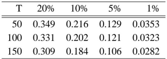
Table 5 Size of the Engle and Hendry test for super-exogeneity.
T 20% 10% 5% 1%
50 0.349 0.216 0.129 0.0353
100 0.331 0.202 0.121 0.0323
150 0.309 0.184 0.106 0.0282
Note: Rejection frequencies for the Engle and Hendry test for✘✚✙✜✛
✁
✬
For comparison purposes, we also consider the Engle and Hendry (1993) test for super-exogeneity. This is a variable addition tests constructed as a conventional
✄
-test for the joint significance of the
in-tervention variables in the conditional model: ✒❑❷ : ✣
❆✑✶ ☎ ✜◆✣
◗☎✶
☎ ✜ ❢ against✒✩❆ : ✣
❆✑✶
☎ ✜❣ and✣ ◗☎✶
☎ ❣✜ ❢P✫
✁
The results for size and power of this test are presented in Tables 5 and 6. Table 5 reports the rejection
frequencies for the test on the conditional model of✒❑❷ :✣
❆✑✶
☎
✜❋✣ ◗☎✶
☎
✜❃❢ against✒✩❆ :✣
❆✑✶
☎
❣
✜ and✣ ◗☎✶
☎
❣✜❃❢
✂
Where✒
✔
✬
✗✄ ✱✚✲✒
✔
✬✆☎✞✝ ✒
✚
✬
❀ and✒
✔
✌✗✄ ✱✚✲✒
✔
✌
☎✞✝ ✒
✚
✌
❀ are the coefficients of the intervention variables in the conditional