www.atmos-chem-phys.net/8/2569/2008/ © Author(s) 2008. This work is distributed under the Creative Commons Attribution 3.0 License.
Chemistry
and Physics
CO measurements from the ACE-FTS satellite instrument: data
analysis and validation using ground-based, airborne and
spaceborne observations
C. Clerbaux1, M. George1, S. Turquety1, K. A. Walker2,3, B. Barret4, P. Bernath2,5, C. Boone2, T. Borsdorff6,
J. P. Cammas4, V. Catoire7, M. Coffey8, P.-F. Coheur9, M. Deeter8, M. De Mazi`ere10, J. Drummond11, P. Duchatelet12, E. Dupuy2, R. de Zafra13, F. Eddounia1, D. P. Edwards8, L. Emmons8, B. Funke14, J. Gille8, D. W. T. Griffith15, J. Hannigan8, F. Hase16, M. H¨opfner16, N. Jones15, A. Kagawa17, Y. Kasai18, I. Kramer16, E. Le Flochmo¨en4,
N. J. Livesey19, M. L´opez-Puertas14, M. Luo20, E. Mahieu12, D. Murtagh21, P. N´ed´elec4, A. Pazmino1, H. Pumphrey22, P. Ricaud4, C. P. Rinsland23, C. Robert7, M. Schneider16, C. Senten10, G. Stiller16, A. Strandberg21, K. Strong3, R. Sussmann6, V. Thouret4, J. Urban21, and A. Wiacek3
1Universit´e Paris 6, CNRS, Service d’A´eronomie/IPSL, Paris, France
2Department of Chemistry, University of Waterloo, Waterloo, Ontario, Canada N2L 3G1, Canada 3Department of Physics, University of Toronto, Toronto, Ontario, Canada M5S 1A7, Canada 4Laboratoire d’A´erologie UMR 5560, Observatoire Midi-Pyr´en´ees, Toulouse, France 5Department of Chemistry, University of York, Heslington, York YO10 5DD, UK 6Forschungszentrum Karlsruhe, IMK-IFU, Garmisch-Partenkirchen, Germany
7Laboratoire de Physique et Chimie de l’Environnement, CNRS, Universit´e d’Orl´eans, Orl´eans, France 8National Center for Atmospheric Research, Boulder, CO, USA
9Spectroscopie de l’atmosph`ere, Chimie Quantique et Photophysique, Universit´e Libre de Bruxelles (U.L.B.), Brussels,
Belgium. P.-F. Coheur is Research associate with the FRS-F.N.R.S, Belgium
10Belgian Institute for Space Aeronomy, Brussels, Belgium
11Department of Physics & Atmospheric Science, Dalhousie University, Halifax, Canada 12Universit´e de Li`ege ULg, Institute of Astrophysics and Geophysics, Li`ege, Belgium 13Department of Physics and Astronomy, State Univ. of New York at Stony Brook, USA 14Instituto de Astrof´ısica, Andaluc´ıa (CSIC), Granada, Spain
15Department of Chemistry, University of Wollongong, Wollongong, New South Wales, Australia 16Institut f¨ur Meteorologie und Klimaforschung, Forschungszentrum Karlsruhe, Germany 17Fujitsu FIP Corporation, Tokyo, Japan
18National Institute of Information and Communications Technology, Tokyo, Japan 19Microwave Atmospheric Science Team, Jet Propulsion Laboratory, CA, USA
20Jet Propulsion Laboratory, California Institute of Technology, Pasadena, California, USA 21Chalmers University of Technology, G¨oteborg, Sweden
22School of GeoSciences, Edinburgh, Scotland
23NASA Langley Research Center, Hampton, Virginia, USA
Received: 19 September 2007 – Published in Atmos. Chem. Phys. Discuss.: 30 October 2007 Revised: 6 May 2008 – Accepted: 6 May 2008 – Published: 16 May 2008
1 2
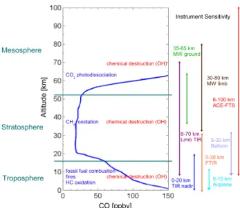
Fig. 1. Schematic plot of a standard atmospheric CO profile, with the different sources of production (blue) and destruction/sinks (red) as a function of altitude. The CO profile was constructed from averaged ACE-FTS data over China and completed with TES data over the same area below 6 km. The vertical sensitivity of each CO sounding type of instrument is also reported on the right-hand side of this plot. MW and TIR refer to millimeter-wave and thermal infrared spectral regions, respectively.
Abstract. The Atmospheric Chemistry Experiment (ACE) mission was launched in August 2003 to sound the atmo-sphere by solar occultation. Carbon monoxide (CO), a good tracer of pollution plumes and atmospheric dynamics, is one of the key species provided by the primary instrument, the ACE-Fourier Transform Spectrometer (ACE-FTS). This in-strument performs measurements in both the CO 1-0 and 2-0 ro-vibrational bands, from which vertically resolved CO con-centration profiles are retrieved, from the mid-troposphere to the thermosphere. This paper presents an updated descrip-tion of the ACE-FTS version 2.2 CO data product, along with a comprehensive validation of these profiles using available observations (February 2004 to December 2006). We have compared the CO partial columns with ground-based mea-surements using Fourier transform infrared spectroscopy and millimeter wave radiometry, and the volume mixing ratio profiles with airborne (both high-altitude balloon flight and airplane) observations. CO satellite observations provided by nadir-looking instruments (MOPITT and TES) as well as limb-viewing remote sensors (MIPAS, SMR and MLS) were also compared with the ACE-FTS CO products. We show that the ACE-FTS measurements provide CO profiles with small retrieval errors (better than 5% from the upper tropo-sphere to 40 km, and better than 10% above). These observa-tions agree well with the correlative measurements, consider-ing the rather loose coincidence criteria in some cases. Based on the validation exercise we assess the following
uncertain-ties to the ACE-FTS measurement data: better than 15% in the upper troposphere (8–12 km), than 30% in the lower stratosphere (12–30 km), and than 25% from 30 to 100 km.
1 Introduction
Carbon monoxide (CO) plays an important role in atmo-spheric chemistry and is one of the key species that needs to be measured globally and at different altitudes. The primary emission sources of CO are associated with combustion pro-cesses (transport, heating, industrial activities and biomass burning), along with biogenic sources and oceans. It is also produced from the oxidation of methane and non-methane hydrocarbons (see Fig. 1). At surface level, the volume mix-ing ratios range from a background concentration of 50 parts per billion by volume (ppbv) to excess of 700 ppbv where high emissions occur. Large uncertainties remain in the es-timated strengths of both natural and anthropogenic sources. The main sink for CO is chemical destruction by reaction with the hydroxyl radical (OH). In the lower atmosphere, where CO has a lifetime of several weeks to a few months, its observation allows the characterization of both emission sources and atmospheric transport of pollution plumes (Lo-gan, 1981). In the upper troposphere, CO can also be trans-ported across the tropical tropopause. In the stratosphere, CO is produced by the oxidation of methane and is converted to carbon dioxide (CO2)by reaction with OH. Above 50 km,
in the mesosphere and thermosphere, photolysis of CO2is
the main source of CO, which reaches a concentration of 5– 20 parts per million by volume (ppmv) at 80 km. At these altitudes, CO is also a useful dynamical tracer which can be used to study atmospheric transport processes, and, in particular, upward transport in high latitude summer regions and downward transport in the high latitude winter regions (e.g. Solomon et al., 1985).
Fig. 2. Microwindows (version 2.2., red lines) used to retrieve CO vertical profiles from the ACE-FTS spectra, for a typical occultation sequence spanning from the free troposphere to the mesosphere. The numbers on the right give the approximate altitude range where the microwindows are valid. The top panel shows a simulated CO spectrum (blue), with the absorption in the 2-0 band multiplied by a factor of 50 for clarity.
are extensive CO observations from space from several nadir looking remote sensors, such as MOPITT/Terra (Edwards et al., 2004; Clerbaux et al., 2008), SCIAMACHY/Envisat (Frankenberg et al., 2005), TES/Aura (Rinsland et al., 2006a; Luo et al., 2007a), and the recently launched IASI/Metop (Turquety et al., 2004; Clerbaux et al., 2007), which are yielding a global view of the CO tropospheric distribution. Although some of them (TES, SCIAMACHY) are also able to partly sound the atmosphere using a limb geometry, their ability to retrieve vertical information is limited. From space, vertically resolved profiles can be derived from measure-ments using limb geometry, in emission or absorption. The currently available limb-sounders working in emission are SCIAMACHY, MIPAS/Envisat (Funke et al., 2007), which uses the mid-infrared spectral range, SMR/Odin (Murtagh et al., 2002) and MLS/Aura (Pumphrey et al., 2007), which both rely on millimeter-wave spectroscopy. In absorption the single instrument currently providing CO measurements is the infrared Atmospheric Chemistry Experiment Fourier
Transform Spectrometer (ACE-FTS) (Bernath et al., 2005). It is worth noting that, among these instruments, only the ACE-FTS is capable of sounding CO simultaneously from the mid-troposphere to the mesosphere.
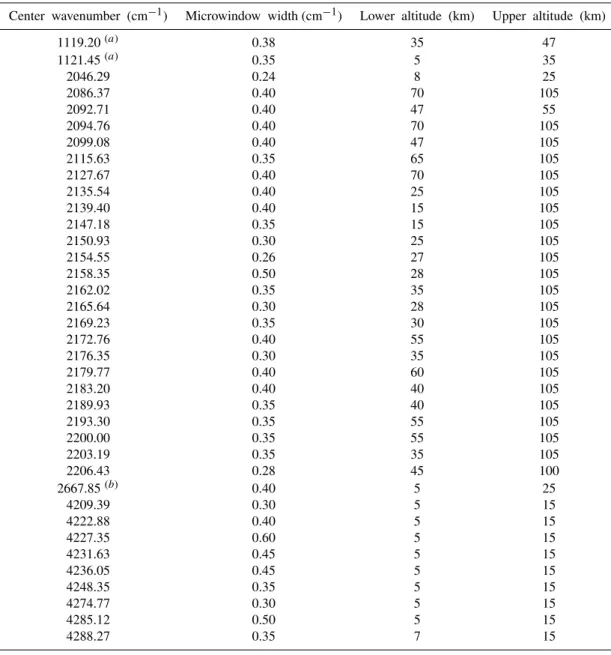
Table 1.Microwindows used for the ACE-FTS CO (main isotopologue) version 2.2 retrievals.
Center wavenumber (cm−1) Microwindow width (cm−1) Lower altitude (km) Upper altitude (km)
1119.20(a) 0.38 35 47
1121.45(a) 0.35 5 35
2046.29 0.24 8 25
2086.37 0.40 70 105
2092.71 0.40 47 55
2094.76 0.40 70 105
2099.08 0.40 47 105
2115.63 0.35 65 105
2127.67 0.40 70 105
2135.54 0.40 25 105
2139.40 0.40 15 105
2147.18 0.35 15 105
2150.93 0.30 25 105
2154.55 0.26 27 105
2158.35 0.50 28 105
2162.02 0.35 35 105
2165.64 0.30 28 105
2169.23 0.35 30 105
2172.76 0.40 55 105
2176.35 0.30 35 105
2179.77 0.40 60 105
2183.20 0.40 40 105
2189.93 0.35 40 105
2193.30 0.35 55 105
2200.00 0.35 55 105
2203.19 0.35 35 105
2206.43 0.28 45 100
2667.85(b) 0.40 5 25
4209.39 0.30 5 15
4222.88 0.40 5 15
4227.35 0.60 5 15
4231.63 0.45 5 15
4236.05 0.45 5 15
4248.35 0.35 5 15
4274.77 0.30 5 15
4285.12 0.50 5 15
4288.27 0.35 7 15
(a)Microwindow for interferer O
3: the mixing ratio profiles of this interfering species are fitted simultaneously with the target CO profile. (b)Microwindow for interferer CH
4: the mixing ratio profiles of this interfering species are fitted simultaneously with the target CO profile.
instruments are outlined. Next, we discuss the comparisons between the ACE-FTS CO data and correlative observations available from March 2004 to December 2006, and, finally, we conclude with the reliability of v2.2 ACE-FTS CO data at different latitudes and altitude levels.
2 CO observations from the ACE-FTS
Table 2.Estimated total error on the retrieved CO partial columns from the ACE-FTS measurements, along with the relative contribution of the instrumental noise. The latter is the main contributor to the error budget. The other contributions include principally uncertainties in the retrieved temperature profiles (a 1 K uncertainty on each retrieval altitude was considered) and fitted interfering species.
Altitude (km) Retrieval error (%) Instrumental noise contribution (%)
6–12 1.9 60
12–25 0.5 71
25–50 0.5 69
50–80 1.1 98
80–100 1.1 96
gases, pressure, and temperature, by solar occultation. The baseline species retrieved from the v2.2 occultation mea-surements are O3, CH4, H2O, NO, NO2, ClONO2, HNO3,
N2O, N2O5, HCl, CCl3F, CCl2F2, HF, and CO (Boone et
al., 2005). While in orbit, the SCISAT instruments observe up to 15 sunrises and 15 sunsets per day. The vertical sam-pling is about 3–4 km, on average, from the cloud tops up to about 105 km. Thanks to its excellent signal-to-noise ratio (effective SNR better than 200–300 over much of its spec-tral range) and 2 s measurement time, ACE-FTS provides accurate measurements with high vertical sampling, but its horizontal resolution is limited by the 500 km path length of solar occultation technique.
2.2 ACE-FTS CO retrievals
The ACE-FTS CO profiles (Boone et al., 2005) are retrieved by analysing sequences of solar occultation measurements taken during a sunrise or sunset, as seen from the satellite. These analyses take advantage of absorptions in both the fun-damental 1-0 (4.7µm) and the overtone 2-0 (2.3µm) CO ro-vibration bands (Clerbaux et al., 2005). Because a large range of optical thicknesses is encountered during a sequence of measurements, the CO retrieval can best be performed us-ing transmittance information from both absorption bands. Figure 2 illustrates the CO spectra as recorded at different tangent altitudes during one ACE-FTS occultation sequence. At high altitudes (>60 km), the CO generated from the CO2
photo-dissociation is the strongest absorber in the 4.7µm spectral range, but the lines saturate at lower tangent heights and the interferences from other atmospheric species (H2O,
O3, N2O, CO2)increase. Both the saturation and the
inter-ferences prevent an accurate tropospheric CO retrieval using this spectral region only.
In the ACE-FTS retrieval process, which uses a global-fit method in a general non-linear least squares minimization scheme (Boone et al., 2005), a set of microwindows that vary with altitude in the fundamental band and in the overtone band are used to retrieve CO. The use of the intense 1-0 band provides information on the upper parts of the atmosphere, whereas the 2-0 band provides information at the lowest
alti-1
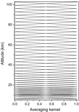
Fig. 3. Typical CO averaging kernels for ACE-FTS, using the mi-crowindows shown in Fig. 2, and an Optimal Estimation Method without a priori constraints. The vertical resolution is∼2 km in the troposphere and 4 km above, for a beta angle of –50.6◦. At low beta angles, the vertical resolution might reach 6 km at the highest altitudes.
2
Fig. 4. ACE-FTS CO seasonal measurements in 2005 at 7.5 km. The data are interpolated to a 4◦latitude×8◦longitude grid. The grey crosses indicate the ACE-FTS measurement locations (tangent heights). The lowest altitude measured by the ACE-FTS varies with the satellite orbit and the presence of clouds.
ratio profiles for these interfering gases are fitted simultane-ously with the target CO profile. The ACE-FTS profiles are provided on a 1-km vertical grid. To obtain the 1-km grid data products, an a posteriori piecewise quadratic interpola-tion scheme method is used to interpolate between the alti-tudes of the original measurement grid. It is worth noting that sometimes the first CO level (at low altitude) should be treated with caution. The v2.2 data products are provided with a fitting error calculated for each altitude. A detailed budget of the retrieval and instrumental errors can be esti-mated (see Clerbaux et al., 2005). It includes contributions from the instrumental noise, from the instrument line shape function, from the so-called smoothing effect (the fact that the information is integrated over several km on the verti-cal), and from uncertainties in the temperature and interfing trace gases profiles. Table 2 summarizes the retrieval er-rors in terms of partial columns, as currently estimated for the ACE-FTS version 2.2 CO retrievals. The error is the largest (2%) for the 6–12 km columns, where the errors due
to interfering species and temperature uncertainties have the strongest impact; it decreases to 0.5% for the 12–25 and 25– 50 km columns and finally increases again to about 1% for the 50–80 and 80–100 km columns. The errors in the indi-vidual retrieved levels of the CO profile is less than 10% in the troposphere (except for the very first levels below 8 km) and the stratosphere, and between 5 and 20% at higher alti-tudes. The measurement noise provides the dominant contri-bution to the error budget over the entire altitude range, with contributions ranging from 60–70% in the upper troposphere and the stratosphere to more than 90% higher up (Table 2). 2.3 ACE-FTS CO distributions
2
Fig. 5. ACE-FTS CO seasonal measurements in 2005 at 16.5 km. The data are interpolated to a 4◦latitude×8◦longitude grid. The grey crosses indicate the ACE-FTS measurement locations (tangent heights). Note that the tropical latitudes are not well covered in January– February–March and October–November–December as the satellite orbit was optimized to study the polar regions in winter.
(Rinsland et al., 2006b, 2007a, 2007b; Coheur et al., 2007; Dufour et al., 2007; Turquety et al., 2008). Previous sci-entific studies have discussed the CO vertical profiles (v1.0 and v2.2) obtained from ACE-FTS since March 2004 (just after scientific commissioning was completed on 21 Febru-ary 2004) (e.g. Clerbaux et al., 2005 (v1.0); Rinsland et al., 2005; Folkins et al., 2006). For CO, version 2.2 provides im-proved performance in the troposphere, as many microwin-dows sensitive to lower altitudes were added to the retrievals. The altitude spacing of the ACE-FTS measurements, con-trolled by the scan time and the orbit of the satellite, varies with the beta angle (the angle between the satellite velocity vector and a vector from the Earth to the Sun). The altitude spacing ranges from 2 km for long occultations with high beta (around 55◦) to 6 km when the sun sets (or rises) exactly perpendicular to the Earth horizon (occultations with beta an-gle zero). Note that the altitude spacing compresses at low altitudes (below about 40 km), primarily a consequence of refraction distorting the solar image viewed through the
at-mosphere. This is clearly seen from Fig. 3, which shows the vertical sensitivity functions, known as averaging kernels, for a typical CO retrieval using an Optimal Estimation Method (Rodgers, 2000) without a priori constraints, such as to re-semble the general least-square retrievals performed opera-tionally for version 2.2. For the particular case of Fig. 3, the vertical sampling is as good as 1.5 km in the troposphere and around 4 km in the mesosphere. There have been improve-ments in the retrievals and averaging kernels near 20–25 km, compared to v1.0 (Clerbaux et al., 2005), due to the com-bined use of the 1-0 and 2-0 ro-vibrational bands to retrieve CO at those altitudes.
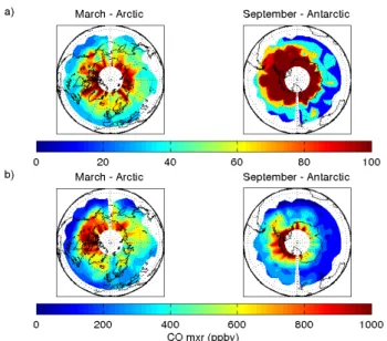
Fig. 6.ACE-FTS CO polar measurements in March and September 2005 at(a)49.5 km and(b)at 59.5 km. The data are interpolated to a 6◦latitude×8◦longitude grid. We used polar projections over the Arctic (left plots) and the Antarctic (right plots) to illustrate the descent of CO-rich air masses in polar vortex situations.
year 2005. The years 2004 and 2006 (not shown here) exhibit similar high concentration values at specific loca-tions/altitudes. Figure 4 illustrates the seasonal CO abun-dance distribution as measured by ACE-FTS in the mid-troposphere (around 7.5 km) for different seasons in 2005. As can be expected (e.g. Clerbaux et al., 2004; Edwards et al., 2004), in the Northern Hemisphere, most of the pollu-tion is associated with urban activity, with persistent high values above China (see Fig. 4b) and elevated levels over US, Europe and Asia in winter and spring (Fig. 4a and b). CO levels are lower in the Northern Hemisphere during sum-mer and fall, when sunlight produces high OH levels which activate chemical loss of CO. In the Southern Hemisphere, the CO pollution plumes emitted locally, where vegetation burning occurs, such as in South America, Africa and Aus-tralia spread from regional to global scales. As reported by others (e.g. http://earthobservatory.nasa.gov/Newsroom/ NewImages/images.php3?img id=17724) intense fire activ-ity and hence high CO levels were observed (starting from September 2005) over the Amazon basin, with some addi-tional contribution from fires in Southern Africa. The trans-ported plume can be observed in Fig. 4c and d, around 30◦S. In the UTLS, vertical transport may be investigated from the satellite CO vertical distributions (Notholt et al., 2003; Edwards et al., 2006; Ricaud et al., 2007; Park et al., 2008). Figure 5 a–d shows the global scale seasonal distributions at 16.5 km altitude, from which the high CO concentrations from convection occurring at tropical latitudes can clearly be seen. The plots illustrate the seasonal changes in convective
outflow and biomass burning activity. From July to Septem-ber (Fig. 5c), when the Asian summer monsoon is the domi-nant circulation feature, high levels of CO are observed over Asia (also see Park et al., 2008). During the other months (Fig. 5b, d), maximum amounts are observed over Africa, South America and Asia, but horizontal transport can be ob-served throughout the tropics.
Figure 6a–b illustrates the strong downward transport of CO-rich air in the winter polar vortex. The CO produced in the lower thermosphere from CO2photolysis is transported
to the middle stratosphere by the mean meridional circulation (Kasai et al., 2005b; Velasco et al., 2007). The plots show the descent of CO-rich air produced around 80 km when vor-tex situations occur, in March over the Arctic pole (Fig. 6, left plots) and in September over the Antarctic (Fig. 6, right plots). A complete discussion of the effects of unusual me-teorological conditions on transport and chemistry for the 2004–2006 period is described in Manney et al. (2008, this Special issue).
3 Correlative CO measurements
3.1 The ACE validation exercise
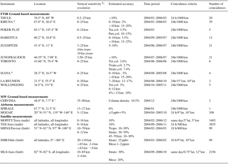
The validation of the ACE-FTS version 2.2 data is organized by data product (see the other papers of this Special issue). CO data from the first three years of the mission, extending from February 2004 (since the first ACE-FTS CO data be-came available) to the end of 2006, were made available to the validation team and are included in this paper. Primarily, the 1-km interpolated grid data were used in the comparisons. Validation data used for these CO comparisons were pro-vided by eleven ground-based stations, from routine airborne measurements, from one accurate high-altitude balloon-borne observation, and from five satellite instruments (two using nadir observations, three using limb-viewing observa-tions). Each instrument uses a different measurement tech-nique, sounding geometry, and dedicated retrieval algorithm (which relies on a forward radiative transfer code, a spec-troscopic database, and a minimization scheme) to extract the desired CO abundances from the raw data (see Table 3). All the instruments reported here used the HITRAN spectro-scopic database (Rothman et al., 2005). Although the HI-TRAN edition might differ, the changes did not concern the CO line parameters and it was verified (E. Mahieu, personal communication) that it did not impact the retrieved results.
Table 3.Ground-based, airborne and satellite instruments used for the ACE-FTS CO validation.
Instrument Location Vertical sensitivityb/ Estimated accuracy Time period Coincidence criteria Number of
resolution coincidences
FTIR Ground-based measurements
THULE 76.5◦N, 68◦W 0.2–25 km <10% 2004/03–2006/03 24 h/1000 km 20 KIRUNAa 67.8◦N, 20.4◦E 0–25 km 0–10 km: 2% 2004/03–2006/03 24h/1000 km 39
>10 km: 15–20%
POKER FLAT 65.1◦N, 147.4◦W 0–24 km Tot col: 3.5% 2004/03 24h/1000 km 5 Part col: 10–15%
HARESTUA 60.2◦N, 10.8◦E 0.5–25 km 0–10 km: 3.5% 2004/09–2005/07 24h/1000 km 12
>10 km: 15–25%
ZUGSPITZE 47.4◦N, 11◦E 3–25 km 5–10% 2004/06–2006/07 24h/1000 km 21
4 km tropo 10 km strato
JUNGFRAUJOCH 46.55◦N, 7.98◦E 3.58–25 km <10% 2004/07–2006/07 24h/1000 km 21 TORONTO 43.66◦N, 79.4◦W 0–25 km Tot col: 2.6% 2004/06–2006/06 24h/1000 km 8
Tropo col: 2.7% Strato col: 7.4%
IZANAa 28.3◦N, 16.5◦W 0–25 km 0–10 km : 2% 2004/08–2005/08 24h/1000 km 4
>10 km: 15–20%
LA REUNION 21.5◦S, 55.5◦E 0–20 km 7–20 km: 12–17% 2004/08–2004/10 24h/15◦lon, 10◦lat 3 WOLLONGONG 34.5◦S, 151◦E 0–25 km Tot col: 3% 2004/10–2005/11 24h/1000 km 5
0–12 km: 4%>12 km: 10%
MW Ground-based measurements
CERVINIA 48.9◦N, 7.7◦Ec 35–90 km Column density: 10.5% 2004/12 24h/1000 km 2
Airborne measurements
SPIRALE 67.7◦N, 21.5◦E 13–27 km 6% 2006/01 24h/1000 km 1
MOZAIC 20◦N–51◦N, 119◦W–140◦E 5–12 km ±5 ppbv+5% 2004/04–2005/10 24 h/9◦lat, 10◦lon 108
Satellite measurements
MOPITT/Terra (nadir) all latitudes, all longitudes 0–16 km 10% 2004/02–2006/12 same day/5◦lat, 5◦lon 3485
TES/Aura (nadir) all latitudes, all longitudes 0–16 km 10% 2004/09–2006/11 24 h/300 km 3855 MIPAS/Envisat (limb) 51◦N–81◦N, 97◦W–180◦E 10–70 km Tropo: 10–30% 2004/02–2004/03 18 h/800 km 99
6–12 km Strato: 30–70%
45–70 km: 10–30%
SMR/Odin (limb) all latitudes, 0◦–186◦E 20–110 km Strato: 25 ppbv 2004/03–2006/02 10 h/9◦lat, 10◦lon 99
<65 km: 2-4 km Meso:1–2 ppmv
>65 km:∼6 km
MLS/Aura (limb) 82◦N–82◦S, all longitudes 10–85 km Strato: 30% 2004/09–2006/10 same day/0.75◦lat, 12◦lon 2156
3–4 km
Meso: 20%
aThese stations use PROFFIT 9.2. version 9 inversion algorithm (Hase et al., 2004), and the retrievals are performed on a log vmr-scale.
All other GB-FTIR stations use SFIT2 inversion algorithm (different versions) (Pougatchev and Rinsland, 1995; Rinsland et al., 1998). Note that both codes were compared in an extensive study, resulting in an agreement of columns of better than 1% (Hase et al., 2004).
bFTIR stations might have some sensitivity higher in the atmosphere, as demonstrated in Velazco et al., (2007).
cLocation for Cervinia measurement is at intersection of slant-angle radiometer beam with 60 km altitude, not station location.
of the instrument with the lowest vertical sensitivity (Rodgers and Connors, 2003):
xsmoothed=xa,low+Alow xhigh−xa,low (1)
wherexhighis the high resolution profile,xa,lowis the a
pri-ori profile used for the retrieval of the low resolution pro-file, andAlowis the averaging kernel matrix, withA=∂xˆ/∂x,ˆ
characterizing the low resolution profiles. The rows ofA de-fine the vertical resolution of the retrieval (full width at half maximum), and the trace of the matrix defines the number of statistically independent elements that can be retrieved, or degrees of freedom for signal (DOFS).
3.2 Ground-based data
Eleven ground-based stations routinely measuring CO pro-files/columns at different locations around the globe con-tributed to this validation exercise. Ten of these stations use FTIR spectrometers to sound the troposphere and lower stratosphere, and one is operating in the millimeter wave spectral range.
3.2.1 FTIR measurements
2
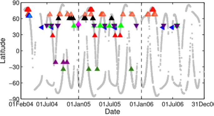
Fig. 7.Geographic locations of the 11 ground-based validation sta-tions used in this paper. Note that there are only two stasta-tions lo-cated in the Southern Hemisphere (La R´eunion and Wollongong), and that four stations are located at latitudes where dynamics can be perturbed by the location of the polar vortex (Thule, Kiruna, Poker Flat, and Harestua).
CO data can be derived (Notholt et al., 2003; Barret et al., 2003; Hase et al., 2004). The FTIR measurements contains about two pieces of information that allow to retrieve CO abundances in the lower to middle troposphere and in the up-per troposphere-lower stratosphere, almost independently.
Figure 7 and Table 3 provide the geographical distribu-tions along with retrieval information for the ground-based ACE-FTS CO validation stations, with the following abbre-viations:
– THULE (Greenland, Goldman et al., 1999), – KIRUNA (Sweden, Blumenstock et al., 2006), – POKER FLAT (Alaska, Kasai et al., 2005a), – HARESTUA (Norway, Paton-Walsh et al., 1997), – ZUGSPITZE (Germanic Alps, Sussmann and
Bors-dorff, 2007),
– JUNGFRAUJOCH (Swiss Alps, Rinsland et al., 2000), – TORONTO (Canada, Wiacek et al., 2007),
– IZANA (Canary Islands, Schneider al., 2005), – LA REUNION (Indian Ocean, Senten et al., 2008), – WOLLONGONG (Australia, Jones et al., 2007). 3.2.2 Microwave measurements
Microwave spectrometers observe molecular rota-tional/vibrational spectra in emission from thermally excited states in the spectral range∼20–300 GHz. They can therefore operate day or night, limited only by tropospheric opacity due primarily to varying water vapour column density. They are not affected by aerosol loading. Since
01Feb04 01Jul04 01Jan05 01Jul05 01Jan06 01Jul06 31Dec06
−90 −60 −30 0 30 60 90
Date
Latitude
Fig. 8. Coincidences between ACE-FTS measurements (in light gray, ACE occultation latitude versus time of year) and the ground based stations, for the three years of the mission. The color code for each station is the same as in Fig. 7. The coincidence criteria are provided in Table 3. Note that if time coincidences occur for a same station, symbols might be superposed.
they observe in emission, they are not self-calibrating, and must be independently calibrated against millimeter sources of known intensity. For the instrument at CERVINIA (de Zafra et al., 2004), when used in a radiometer mode to get total column density, this calibration uncertainty, along with uncertainty in continuous measurements of tropospheric attenuation, are the only significant sources of error. For this instrument, observations are made at a slant angle of 9–10 degrees in a due north direction, giving a stratospheric/mesospheric point of intersection about 3 degrees north of the ground station location, and this has been used in considering closest matches with ACE-FTS measurements. The location of this station, in the Italian alps, and the retrieval details are also reported in Fig. 7 and Table 3.
3.3 Airborne data
3.3.1 SPIRALE (high altitude balloon)
1
0
50
100
150
0
5
10
15
20
25
30
CO [ppbv]
Altitude [km]
−50 −20 0 20
50
0
5
10
15
20
25
30
Percent
0
50
100
150
0
5
10
15
20
25
30
CO [ppbv]
−50 −20 0 20
50
0
5
10
15
20
25
30
Percent
0
50
100
150
0
5
10
15
20
25
30
CO [ppbv]
Altitude [km]
−50 −20 0 20
50
0
5
10
15
20
25
30
Percent
0
50
100
150
0
5
10
15
20
25
30
CO [ppbv]
−50 −20 0 20
50
0
5
10
15
20
25
30
Percent
ACE−FTS
ACE−FTS smoothed JUNGFRAUJOCH
21 obs.
ACE−FTS
ACE−FTS smoothed KIRUNA 39 obs.
ACE−FTS
ACE−FTS smoothed THULE 20 obs.
ACE−FTS
ACE−FTS smoothed ZUGSPITZE 21 obs.
2
3
Fig. 9. Left panel, for each ground-based (GB) station (Jungfraujoch, Kiruna, Thule and Zugspitze): Averaged CO mixing ratio profiles and variability for ACE-FTS (in blue: raw data, in red: after treatment with the corresponding ground-based averaging kernels) and for the collocated corresponding ground-based measurements (green). Right panel, for each ground-based station : averaged percent difference between ACE-FTS and GB (COACE–COGB/1/2(COACE+COGB))calculated for all the coincident observations (thick line), along with their standard deviation (thin lines).
two cell mirrors give a total optical path of 430.78 m. Species concentrations are retrieved from direct infrared absorption, by fitting the experimental spectra to spectra calculated using the HITRAN 2004 database (Rothman et al., 2005). Specifi-cally, the ro-vibrational line at 2086.3219 cm−1was used for CO.
3.3.2 MOZAIC (airplane)
The MOZAIC program (Marenco et al., 1998) has equipped five commercial airliners with instruments to measure ozone and relative humidity since 1994, and carbon monoxide since 2001. Measurements are taken from take-off to land-ing (Thouret et al., 1998). Based on an infrared analyser, the carbon monoxide measurement accuracy is estimated at±(5 ppbv+5%) for a 30 s response time (Nedelec et al.,
2003). The five MOZAIC aircraft make near-daily flights between Europe and a variety of destinations throughout the world. Measurements for more than 26 000 long-haul flights are recorded in the MOZAIC data base that is freely acces-sible for scientific use (URL: http://mozaic.aero.obs-mip.fr/ web/).
3.4 Nadir-looking satellites 3.4.1 MOPITT/Terra
Table 4.Averaged percent difference and standard deviation between ACE-FTS and each ground-based (GB) station. The calculation was done for partial CO columns, for each coincident set of profiles using (100×|(COACE–COGB)|)/1/2 (COACE+COGB). Values in italics correspond to the calculation after smoothing with the GB averaging kernel functions. Values in parentheses correspond to calculation after filtering situations for which different air masses might have been sounded.
Ground-based station Averaged relative difference (%) Standard deviation (%)
THULE 37.1 (30.8) 29.7 (21.5)
26.5 (21.4) 28.3 (15.4)
KIRUNA 31.3 (31.2) 24.2 (23.8)
28.9 (28.3) 16.5 (16.4)
POKER FLAT 20.0 14.6
15.6 8.5
HARESTUA 40.4 (39.6) 29.5 (32.3)
19.0 (19.9) 16.7 (18.3)
CERVINIA 25.8 31.5
ZUGSPITZE 22.5 21.7
24.3 21.6
JUNGFRAUJOCH 16.7 10.5
16.3 10.9
TORONTO 24.5 11.2
33.7 23.0
IZANA 13.2 8.9
13.1 6.9
LA REUNION 18.5 15.3
13.3 6.9
WOLLONGONG 23.8 14.8
27.0 24.7
approximately 98.2 degrees. The descending node crossing time is 10:30 a.m. MOPITT views the Earth over all latitudes with a pixel size of 22 km by 22 km and a cross-track swath that provides a near-global measurement of the distribution of CO every three days.
MOPITT operates by sensing infrared radiation from ei-ther the ei-thermal emission/absorption at 4.7µm to measure CO profiles. The measurement technique exploits gas corre-lation radiometry to determine tropospheric concentrations. Operational MOPITT CO products available are currently based exclusively on thermal-channel radiances (Deeter et al., 2003; Emmons et al., 2004). The information content in MOPITT retrievals is better than a column in tropical and mid-latitude scenes, with some amount of profile shape in-formation (DOFS between 1 and 1.8), and a maximum sen-sitivity around 5–8 km (Deeter et al., 2004). As the other thermal infrared instruments, MOPITT generally lacks sensi-tivity near the surface except during daytime and at locations where the thermal contrast (temperature gradient) between the surface and lower atmosphere is significant (Clerbaux et al., 2008).
This paper uses the version 3 retrievals from NASA Lang-ley.
3.4.2 TES/Aura
The Tropospheric Emission Spectrometer (TES) is an in-frared FTS on board the EOS Aura satellite launched in July 2004 (Beer, 2006). TES routinely operates in a nadir global survey mode with one-day-on followed by one-day-off cy-cles. The nadir footprint for a TES profile is 5 km×8 km, separated by 180 km along orbit, since May 2005. TES nadir spectra are recorded at 0.06 cm−1resolution and small micro-windows in the CO (1-0) band are used for CO pro-file retrievals. The signal levels in the TES filter detecting CO spectral absorptions are greatly enhanced due to the im-proved optical alignment after an optical bench warm-up per-formed in December 2005. As a result, the DOFS and the precision in TES CO retrievals are improved (Rinsland et al., 2006a). The DOFS for TES CO are up to two in the tropics and become less than one at high latitudes.
0 0.02 0.04 0.06 0.08 0.1 0
0.02 0.04 0.06 0.08 0.1
FTIR [x1019 molecules/cm2]
ACE−FTS [x10
19
molecules/cm
2 ]
THULE
KIRUNA
POKER FLAT
HARESTUA
CERVINIA
ZUGSPITZE
JUNGFRAUJOCH TORONTO
IZANA
LA REUNION
WOLLONGONG
Fig. 10.Scatterplot of the ground-based CO partial column obser-vations and the corresponding ACE-FTS CO partial columns calcu-lated after treatment of profiles with the GB averaging kernel func-tions (except for the Cervinia station). The ground-based stafunc-tions are identified by different colors (see legend). Each partial column is obtained by integration of the CO concentration from the low-est available ACE-FTS level (typically 6.5–8.5 km) to the altitude indicated in Table 3. Density profiles were obtained by interpolat-ing of ECMWF temperature and pressure fields to match the time and location of each measurement. Special symbols (star) are used when the calculated values are believed to correspond to signifi-cantly different airmasses, in polar vortex situations (see text). The correlation coefficient is 0.91 (slope 0.86, intercept 0.0019).
3.5 Limb-viewing satellites 3.5.1 MIPAS/Envisat
The Michelson Interferometer for Passive Atmospheric Sounding (MIPAS) is a limb emission FTS operating in the mid infrared spectral region (Fischer et al., 2008). It is part of the Environmental Satellite (Envisat) which was launched into its sun-synchronous polar orbit, with 98.55◦inclination at about 800 km altitude, in March 2002. MIPAS operated from July 2002 to March 2004 at full spectral resolution (0.035 cm−1). Within this standard observation (nominal) mode, MIPAS covered the altitude range from 6 to 68 km with tangent altitudes from 6 to 42 km every 3 km, and fur-ther tangent altitudes at 47, 52, 60, and 68 km. MIPAS passes the equator in southerly direction at 10:00 a.m. solar local time 14.3 times a day. During each orbit up to 72 limb scans are recorded.
Vertical profiles of CO are among the 20 trace species re-trieved with the dedicated scientific IMK-IAA MIPAS data processor (von Clarmann et al., 2003). CO 1-0 emissions at
0 50 100 150 10
12 14 16 18 20 22 24 26 28 30
CO [ppbv]
Altitude [km]
−100 −50 0 50 100 10
12 14 16 18 20 22 24 26 28 30
Relative Difference [%]
ACE−FTS
2006−01−21 64.3°N, 21.6°E
SPIRALE
2006−01−20 67.7°N, 21.6°E
Fig. 11. Left: Averaged CO mixing ratio profile for ACE-FTS (blue) and for the co-located SPIRALE measure-ments (green). Right: The red line is the COACE– COSPIRALE/1/2(COACE+COSPIRALE)percentage difference.
4.7µm, strongly affected by non-local thermodynamic equi-librium (non-LTE) effects, are used in the retrieval scheme which fully accounts for non-LTE (Funke et al., 2007). In this study, we used MIPAS CO data (version 9.0) retrieved from MIPAS standard observations taken at full spectral res-olution (spectra versions 4.61 and 4.62) during February– March 2004. The MIPAS vertical resolution varies between 6 and 12 km.
3.5.2 SMR/Odin
The Odin satellite was launched in February 2001 into a cir-cular, sun-synchronous, quasi-polar orbit at 600 km altitude, with an inclination of 97.8◦and ascending node crossing at 18:00 local time (Murtagh et al., 2002). The Sub-Millimetre Radiometer (SMR) aboard Odin measures thermal emission lines at the Earth’s limb in the 486–581 GHz spectral range (Frisk et al., 2003). Measurements of CO and O3in the SMR
strato-mesospheric mode (vertical scan range of 7–110 km) are performed regularly (one or two days per month since 2004) by observing rotational lines at 576.27 GHz (CO) and 576.52 GHz (O3). The horizontal resolution is on the order
of 600 km, with a horizontal spacing along the orbit track of
∼950 km.
0 50 100 150 0
5 10 15 20 25 30
CO [ppbv]
Altitude [km]
0 50 100 150
0 5 10 15 20 25 30
CO [ppbv]
Altitude [km]
ACE−FTS
2004−09−03 50.9°N, 6.4°E MOZAIC
2004−09−03 50.3°N, 7.1°E
ACE−FTS
2005−05−04 43.6°N, 13.2°W MOZAIC
2005−05−04 44.5°N, 20.7°W
2 3
Fig. 12. Examples of co-located CO vertical mixing ratio profiles measured by ACE-FTS (blue) and by the MOZAIC airborne pro-gram (green). Note that the upper limit altitude of the MOZAIC measurement is often close to, or at the same altitude, as the ACE-FTS lowest measured altitude.
estimated at better than 25 ppbv in the stratosphere increas-ing up to 1–2 ppmv at ∼80 km (Barret et al., 2006). The SMR CO measurements and data analysis methodology were described in detail by Dupuy et al. (2004). Early qualita-tive comparisons with ACE-FTS were published by Jin et al. (2005), whilst a detailed comparison of SMR/Odin with Aura/MLS can be found in Barret et al. (2006).
3.5.3 MLS/Aura
The Microwave Limb Sounder (MLS) (Waters, 2006) is one of four instruments on the EOS Aura satellite (Schoe-berl et al., 2006) which was launched in July 2004. MLS is essentially a small radio telescope, viewing the Earth’s limb in the orbit plane of the Aura satellite. Observations range from 82 degrees South to 82 degrees North every day and are spaced 140 km apart along the ground track. MLS detects thermally-emitted radiation in several bands of the sub-millimetre spectral region, at frequencies ranging from 118 GHz to 2500 GHz. The measurements are processed to obtain profiles of temperature, geopotential height and the mixing ratio of more than 14 chemical species.
The mixing ratio of CO is obtained from measurements of the spectral line at 230 GHz. Two separate spectrometers are centred on this spectral line: a conventional filter bank of 25 channels and a digital autocorellator spectrometer (DACS) with 129 channels. The DACS channels are 97.6 kHz wide giving a total width of 12.5 MHz. The conventional filter bank has channels of various widths ranging from 6 MHz to 96 MHz, giving a total bandwidth of over 1 GHz. Version 2.2 data products are used for these comparisons. The MLS retrieval technique is described in detail by (Livesey et al.,
−40 −20 0 20 40 6
7 8 9 10 11 12
Relative Difference [%]
Altitude [km]
Fig. 13. Averaged percent difference between ACE-FTS and MOZAIC (COACE–COMOZAIC/1/2(COACE+COMOZAIC)), calcu-lated using all the coincident observations (thick red line), along with the corresponding standard deviation (thin red lines) for the years 2004 and 2005. The number of coincident profiles ranges be-tween 4 (at 12 km) to 37 (at 8–9 km).
2006) and the validation of the 2.2 CO product is provided in (Pumphrey et al., 2007).
4 Validation results
4.1 Methodology used for the intercomparison
All the data used in this paper were obtained from the teams that are working on the routine retrieval and analysis of CO concentrations for their measurement device, and who helped us to select the most reliable data for the validation comparisons. The coincidence location criteria (ACE-FTS versusinstrument) and the CO product to compare (profile, smoothed profiles, or integrated partial columns) were de-cided in agreement with the participants, and after discussion with the people involved in the validation of the ACE-FTS products, for consistent analyses.
In this paper, we used the same procedure to treat all the measurements provided by the participating groups:
1. Select the data that meet the location and time coinci-dence criteria (see Table 3),
2. Intercompare ACE-FTS versus instrument at the alti-tude range where both instruments are simultaneously sensitive,
0 50 100 150 6 8 10 12 14 16 18 20 CO [ppbv] Altitude [km]
0 50 100 150
6 8 10 12 14 16 18 20 CO [ppbv] Altitude [km] ACE−FTS 2005−08−18 35.4°S,167.5°W ACE−FTS smoothed MOPITT 2005−08−18 34.3°S,170.7°W ACE−FTS 2005−07−22 57.3°N,174°E ACE−FTS smoothed TES 2005−07−22 57.3°N,171°E 2 3
Fig. 14. Examples of co-located CO vertical mixing ratio profiles for ACE-FTS (blue) and two nadir-looking instruments (green): MOPITT (left) and TES (right). The retrieval errors are also re-ported (horizontal blue bars show ACE-FTS fitting errors from v2.2, and horizontal green bars at each retrieved level for the nadir-looking instrument). The red curve represents the convolution of the ACE-FTS profile with the averaging kernel function of the nadir-viewing instrument.
4. Calculate the percent difference COACE
-COinst rument/1/2(COACE+COinst rument), averaged over all the coincident observations, and the corre-sponding standard deviation,
5. Check if the co-location criteria used are stringent enough to sound similar air masses (for polar cases). 4.2 Ground-based data
A summary of the number of coincidences with ACE-FTS occultation measurements (for which ACE-ACE-FTS CO re-trievals were available) is given in Table 3 for each ground-based station, along with an indication of the vertical sen-sitivity of the observation and the associated accuracy. A more complete description of each station, instrument and CO retrieval setup (inversion algorithm used and spectro-scopic databases) can be found in the above-mentioned ref-erences (Sect. 3.2). After some tests, the coincidence criteria were chosen such that the measurements were within 24 h and within 1000 km. This ensured that there were at least a few matches per station. In case several ground-based pro-files were available for one ACE occultation, the one that oc-curred closest in time was chosen. Figure 8 illustrates the time and location coincidences between the ACE occulta-tion measurements and each of the ground based staocculta-tions for February 2004–December 2006.
For the ground-based stations, the number of coincident CO observations was found to vary between 2 and 39, de-pending on the location of the station, the frequency of
ACE-−60 −40 −20 0 20 40 60 5 6 7 8 9 10 11 12 13 14 15
Relative Difference [%]
Altitude [km]
−40 −20 0 20 40 5 6 7 8 9 10 11 12 13 14 15
Relative Difference [%]
Altitude [km]
MOPITT TES
2 3
Fig. 15. Averaged percent difference (COACE -COnadir/1/2(COACE+COnadir)), calculated using all the coin-cident observations (thick blue line), along with the corresponding standard deviation (thin blue lines) for the years 2004, 2005 and 2006 (left, MOPITT) and 2005–2006 (right, TES). The red lines are for the ACE-FTS profiles which are smoothed by the nadir sounder averaging kernel functions. For both instruments, the number of coincident profiles ranges between∼850 (at 6 km) to
∼3400 (above 12 km).
FTS measurements at the latitude of the station and the cloud coverage. A smoothing of the ACE-FTS CO profiles was also performed according to Eq. (1), using the a priori pro-files and averaging kernel functions provided along with the ground-based CO profile observations.
01Feb04 01Jul04 01Jan05 01Jul05 01Jan06 01Jul06 31Dec06 −90
−60 −30 0 30 60 90
Date Latitude ACE
MIPAS SMR/Odin MLS
2
Fig. 16. Coincidences between the ACE-FTS measurement loca-tions (in light gray, ACE occultation latitude versus time of the year) with the limb satellite measurements (MIPAS in magenta circles; SMR as green triangles; MLS in blue circles) in 2004, 2005 and 2006. The coincidence criteria are provided in Table 3. Note that if time coincidences occur for a same station, symbols might be superposed.
later, so some variability in the CO content is to be expected. When looking at Fig. 10 and Table 4, the largest disagree-ments and standard deviations are observed over stations lo-cated at very high latitudes and hence where measurements may sample different regions of the polar vortex. For ob-servations at high latitudes that were measured close to or within the polar vortex, further investigation was performed in order to check if both the validation and the ACE-FTS in-strument have sounded the same air masses. For these cases, potential vorticity (PV) maps in the region of both measure-ments were calculated using the MIMOSA contour advection model (Hauchecorne et al., 2002), on isentropic surfaces at 475 K (∼18 km) and the air masses were compared. The data potentially coming from different air masses are flagged with a different symbol (star) in Fig. 10 and the calculations of relative differences in Table 4 are provided with and without accounting for these specific situations.
4.3 Airborne data
4.3.1 SPIRALE (high altitude balloon)
Only one coincidence (Fig. 11) was found with the SPI-RALE balloon measurements and it occurred on 20 January 2006 between 17:32 UT and 19:47 UT. The CO volume mixing ratio profile was obtained during ascent, between 10.0 and 27.3 km. The balloon measurement position re-mained rather constant, with a mean location of 67.6±0.2◦N and 21.55±0.20◦E. The comparison is made with the ACE-FTS sunrise occultation that occurred 13 h later (sr13151 on 21 January 2006 at 08:00 UT, 64.28◦N, 21.56◦E) and 413 km away from the SPIRALE position.
Similar to what was performed for ground-based stations, a potential vorticity map was calculated from the MIMOSA contour advection model in the region of both measurements.
They show that SPIRALE and ACE-FTS sounded similar air masses within the well-established polar vortex for the whole range of altitudes. The dynamical situation was stable with the PV agreement obtained to better than 10%. Even though ACE-FTS has a vertical resolution of 3–4 km and that of SPIRALE is more of the order of meters, smoothing the lat-ter data with a set of triangular convolution functions (each 3 km at the base corresponding to the ACE resolution) did not change the shape of the SPIRALE CO profile.
For CO, the SPIRALE total uncertainty is estimated to be 6% over the entire altitude range. As shown in Fig. 11, the agreement is better than 22% between SPIRALE and ACE-FTS profiles for the altitude range 14–20 km. Be-tween 20 and 24 km, the ACE-FTS profile is lower than SPI-RALE by 36–120%. Above 24 km, the ACE-FTS profile be-comes larger than SPIRALE with relative differences reach-ing 120% around 26–27 km. Although the SPIRALE instru-ment is providing more accurate measureinstru-ments than ACE-FTS, it is difficult to draw conclusions based on a single win-ter profile located 400 km away and measured within the po-lar vortex. The ACE-FTS high positive values around 27 km might also be related to the negative ones around 23 km. 4.3.2 MOZAIC (airplane)
The CO measurements recorded during the MOZAIC com-mercial flights in 2004 and 2005 were compared with the ACE-FTS data. The collocation criteria, within 24 h and within a geographic distance of±9◦latitude and±10◦ lon-gitude, provided 108 matches. As there is only a small height range (localized between 6 and 12 km) where the CO mea-surements from both instruments overlap, we added an extra constraint such that at least three km of common observations should exist. The number of available co-located observa-tions then decreased to 39. Figure 12 illustrates two typical examples where the highly resolved MOZAIC CO profiles connect well with the ACE-FTS data. Figure 13 summarizes comparisons between the two datasets for 2004 and 2005, by plotting the average of the percentage relative difference between the coincident ACE-FTS and MOZAIC data. The standard deviation of the differences is also provided, along with the number of data points used at each altitude. The agreement is very good, as the averaged difference is found to be lower than 16% between 6 and 12 km, in 2004–2005, with a positive bias. A parallel work performed with other airborne data (Hegglin et al., 2008) reports a 10% agreement for CO in the same altitude range.
4.4 Nadir-viewing satellites: MOPITT/Terra and TES/Aura
0
50
100
150
0
10
20
30
40
50
60
70
80
CO [ppbv]
Altitude [km]
0
50
100
150
0
10
20
30
40
50
60
70
80
CO [ppbv]
0
50
100
150
0
10
20
30
40
50
60
70
80
CO [ppbv]
ACE−FTS
2004−03−25 56.4°N,85.4°E
ACE−FTS smoothed
MIPAS
2004−03−25 61.1°N,98.3°E
ACE−FTS
2004−09−18 78.6°N,171.3°E
SMR/Odin
2004−09−18 71.7°N,174.4°E
ACE−FTS
2006−01−20 64.1°N,52.5°E
MLS
2006−01−20 64.7°N,56.6°E
Fig. 17.Examples of co-located CO vertical mixing ratio profiles for ACE-FTS (blue) and three limb-looking instruments (MIPAS, SMR and MLS; in green). The retrieval errors are also reported (horizontal blue bars for ACE-FTS fitting errors from v2.2 files, and horizontal green bars for each limb-instrument). As MIPAS data are less vertically resolved, the ACE-FTS profile was smoothed by the MIPAS averaging kernels (in red).
Table 5. Summary of percent average difference on partial columns for the validation instruments, as a function of altitude, using (100 x (COACE–COI nst ru)/1/2 (COACE+COI nst ru). When a smoothing was applied, data are provided in italics.
Altitude range (km) Instrument
GB SPIRALE MOZAIC MOPITT TES MIPAS SMR MLS
06–12
13–34%
+15.5% –25.2% ±17.9% ±22.1%
(altACE–25 km)
–2.2% ±1.3% ±22.9%
(5.5–13.6 km) (6–14 km)
12–20 –21.1% –11.4% –88.8% –54.6%
(14–20 km) –20.1%
20–30 110.4% +26.4% ±17.7% >±200%
(20–27 km) +8.0%
30–50 –27.2% –3.5% ±84.2%
±18.6%
50–80 –22.9% +24.7% ±104.4%
–5.3%
0 50 100 150 0
5 10 15 20 25 30
CO [ppbv]
Altitude [km]
0 50 100 150
0 5 10 15 20 25 30
CO [ppbv]
0 50 100 150
0 5 10 15 20 25 30
CO [ppbv]
−100−50 0 50 100
0 10 20 30 40 50 60 70 80
Relative Difference [%]
Altitude [km]
0 100
Nb of obs.
−100−50 0 50 100
0 10 20 30 40 50 60 70 80
Relative Difference [%]
0 100
Nb of obs.
−100−50 0 50 100
0 10 20 30 40 50 60 70 80
Relative Difference [%]
0 2000
Nb of obs.
MIPAS
SMR/Odin
MLS
Fig. 18. Top panel: CO mixing ratio profiles, averaged over all the coincident observations, for ACE-FTS (blue) and three limb-viewing instruments (in green). The standard deviations are plotted as horizontal bars.ACE-FTS smoothed by the MIPAS averaging kernel functions is plotted in red. Bottom panel: Averaged percent difference (COACE–COlimb/ 1/2(COACE+COlimb), thick lines), along with the corre-sponding standard deviation (thin lines) for MIPAS (before and after smoothing ACE-FTS, in blue and red respectively), SMR and MLS. The number of data points included in the average, as a function of altitude, is also provided as sub-plots.
size and global coverage, coincidences with the ACE-FTS occultation measurements are numerous. This study was per-formed using the following criteria: same day and within 5◦ longitude, 5◦latitude for MOPITT (version 3), and±24 h, within 300 km for TES (version V002). The choice of the coincidence criteria depended on how the data products are
stored for each mission. For both instruments more than 3000 cases were found, spanning 2004, 2005 and 2006.
they provide have a limited vertical resolution. Although the CO volume mixing ratio products are provided at several al-titudes, the levels are strongly correlated and the number of pieces of independent information ranges between one (to-tal column) and two (two partial columns), depending on the latitude, with a maximum sensitivity in the free troposphere and information up to about 16 km. As discussed in Luo et al. (2007a), both MOPITT and TES CO retrieved profiles are biased by their a priori; but when similar initial conditions are considered, TES and MOPITT agree reasonably (<5% global average with<20% root mean squares for individual cases). Accuracies for both instruments were estimated to be 10% using aircraft data (Emmons et al., 2004; Luo et al., 2007b), in places where the retrievals are not influenced by the a priori.
Interestingly, as MOPITT and TES both have their max-imum sensitivity around 6–8 km, a useful comparison can be obtained in the upper troposphere. In order to account for the different vertical sensitivities in the comparisons, the ACE-FTS profiles have been smoothed using the correspond-ing MOPITT and TES characteristics and Eq. (1). Figure 14 shows one MOPITT/ACE-FTS and one TES/ACE-FTS ex-ample comparison of co-located profiles used in the valida-tion exercise. It can be seen that, here again, we have only a few altitude levels in common between the measurements (ACE-FTS profiles start no lower than 5 km). As expected, when looking at the paired sets of observations, the ACE-FTS CO profiles show much more vertical variability, with often the 5–10 km CO mixing ratios being higher, and the 10–20 km CO mixing ratio being lower than the MOPITT or TES ones. As can be observed from Fig. 14, the smoothed ACE-FTS profiles match the nadir viewing observations very well. Figure 15 provides the mean and standard deviation re-sults averaged for the thousands of coincident profiles stud-ied for the period 2004–2006. For both instruments, without smoothing, the agreement is around 10% between 5.5 and 8.5 km, and the disagreement increases with a negative bias of –10 to –60% for MOPITT and around –25% for TES in the range 9 to 15 km. As MOPITT relies on a single global a pri-ori whereas TES uses different latitude-varying a pripri-ori, we expected to find higher differences in the case of MOPITT. After convolution with the averaging kernels associated with each instrument, we have an almost perfect match (less than 2.2% discrepancy in the 5.5–15 km altitude range). Differ-ences in retrieval diurnal sensitivity are also accounted for this way.
4.5 Limb-viewing satellites: MIPAS/Envisat, SMR/Odin and MLS/Aura
There are currently three spaceborne instruments provid-ing regular CO measurements usprovid-ing limb geometry: MI-PAS/Envisat (Funke et al., 2007), SMR/Odin (Barret et al., 2006) and MLS/Aura (Filipiak et al., 2005). As for ACE, these missions are not able to see the lowest layers of the
1
−1 0.01 0.02 0.05 0.1 0.2 0.5 1 2 5 10 20 50
−80 −40 0 20 40 60
20 40 60 80
Latitude
Approx Altitude / km
−1 0.01 0.02 0.05 0.1 0.2 0.5 1 2 5 10 20 50
−80 −40 0 20 40 60
20 40 60 80
Latitude
Approx Altitude / km
2
3
Fig. 19. ACE-FTS (top) and MLS (bottom) CO mixing ratios (ppmv) for 2 September–13 October 2006. For ACE-FTS the sun-set latitude moves northwards during this period, so 2 September is at the left-hand side of the Figure. The ticks near the bottom of the Figure show the mean ACE-FTS latitude for each of the days plotted; the length of each tick is proportional to the number of ACE-FTS sunset profiles on that day. For each ACE-FTS sunrise profile we took the 5 closest collocated MLS profiles and average together all such profiles for the day, in order to reduce noise. The data have been smoothed in latitude, with a smoothing length of 3◦.
atmosphere due to the increase in atmospheric opacity and occurance of clouds.
A detailed validation study of SMR versus MLS is found in (Barret et al., 2006), and a detailed comparison of MLS CO results with other instruments is provided in (Pumphrey et al., 2007).
instrument indicated. When several observations matched the same ACE-FTS profile, we selected the closest in time.
For MIPAS, the CO measurements available (version 9.0) just overlapped with the beginning of the ACE mission. By the end of March 2004, MIPAS operation was suspended due to instrumental problems. MIPAS resumed its mea-surements by the beginning of 2005, however, with reduced spectral resolution. For comparison with ACE-FTS, only the high-resolution data are chosen. In the MIPAS sensi-tive range (10–70 km), the vertical resolution varies between 6 and 12 km, depending on altitude region and illumination conditions. The estimated precision is 10–30% except for the 20–45 km region with values around 30–70%. The accu-racy is limited mainly by instrumental noise. Model errors due to uncertainties in the non-LTE modelling have been es-timated to be less than 10% (Funke et al., 2007). During the February and March 2004 period, using a coincidence crite-rion of (±18 h,±1000 km), about 100 matches were found. It is worth noting that a very strong polar vortex occurred in the 2004 Arctic winter, leading to downwelling of large amounts of CO into the upper stratosphere. The convolution of ACE-FTS profiles with MIPAS averaging kernel functions was found to be necessary, as MIPAS vertical resolution is lower than that of ACE-FTS, in particular during night and above 40 km.
For SMR CO observations, we used the data (CTSO, ver-sion 225) as described in Barret et al. (2006), with the fol-lowing coincidence criteria: ±10 h,±9◦latitude and±10◦ longitude. A quality filter to select the more reliable data (good convergence and measurement response over 75%) led to 99 coincidences, with a vertical sensitivity from∼20 to 95–100 km, and an average vertical resolution of∼3 km.
The largest set of validation data is provided by the MLS/Aura instrument. More than 2100 coincidences were found using the following criteria: same day, ±0.75◦ lat-itude, ±12◦ longitude. Following the recommendations from Pumphrey et al. (2007), the MLS data (version 2.2.) were filtered using the following values for internal checks: L2gpPrecision>0; and Quality>0.2; and Status<126; and Convergence<1.8. The vertical sensitivity of MLS ranges from 10 to 85 km, with 3–4 km vertical resolution over most of this range.
Typical CO profiles for each limb-viewing instrument are compared with the corresponding ACE-FTS CO data in Fig. 17. In general, the agreement per set of profiles is rea-sonable, depending on the altitude level considered. The ACE-FTS CO profiles are usually smoother than SMR and MLS (see Pumphrey et al., 2007 for further discussion), but the ACE-FTS v2.2 sometimes show oscillations (with even negative values) around 40–50 km, which might lead to large discrepancies when comparing with the other limb instru-ments at these altitudes.
Figure 18 provides the averaged profiles, the relative dif-ferences, the standard deviations and the number of coinci-dences per altitude, over the whole data set for each
instru-ment. When looking at the relative difference plots, for MI-PAS (Fig. 18, bottom left plot) the agreement is very good. After smoothing with the averaging kernel, the differences between the convolved ACE-FTS and MIPAS profiles (red line) are within±26% at all altitudes, except between 38 and 41 km where it reaches –50%. These differences are linked to the very unusual situation of strong CO-downward transport in the Artic polar vortex in 2004, where most of the coin-cidences between ACE-FTS and MIPAS are located. When all the data above 70◦N are filtered out, the differences were found to be further reduced (not shown here), but the number of coincident data decreased from 99 to 27.
SMR CO mixing ratios (Fig. 18, bottom middle plot) are considerably larger than those of ACE-FTS (by more than 50%) below∼22 km. Between 25 and 68 km, we found a very good agreement as the difference does not exceed 25%. Above 60 km, the ACE-FTS mixing ratios become larger than the SMR values.
For MLS, we found a negative bias below 20 km, large os-cillating discrepancies between 20 and 35 km, a good agree-ment between 38 and 42 km, a negative bias ranging from –25% to –100% from 42 to 65 km, and a strong positive bias between 65 and 80 km.
Several studies comparing CO measured by the ACE-FTS, SMR and MLS limb sounders have already been published (Froidevaux et al., 2006; Barret et al., 2006; Pumphrey et al., 2007). Our results are broadly consistent with those studies however the plots might look different because we used 1/2 (COACE+ COlimb) to calculate the relative values, instead of
(COlimb) as was used in the above-mentioned papers. In the
upper troposphere (below 20 km), we found that ACE-FTS CO profiles are much lower than those of MLS and SMR, in agreement with the results from Pumphrey et al. (2007) who have compared MLS version 2.2 and ACE-FTS CO. Livesey et al. (2008) also show that MLS CO is a factor of 2 too high at the 215 hPa retrieval level by comparison with MOZAIC airborne in situ data. In the lower stratosphere (below 30 km) ACE-FTS exhibits an underestimation of CO relative to MLS which is consistent with Pumphrey at al. (2007) and Froide-vaux et al. (2006). Barret et al. (2006) reported an underesti-mation of MLS CO relative to SMR, especially in the tropics, at these altitudes.
5 Summary and conclusions
This paper provides an assessment of the CO atmospheric profiles obtained during the first three years of the ACE mis-sion, in order to quantify the level of agreement obtained with other available instruments. The ACE-FTS CO version 2.2 products are derived from solar occultation measurements, using two CO absorption bands located around 2100 cm−1 and 4250 cm−1, which allows sounding the atmosphere from about 5 km up to 100 km. The vertical sampling ranges from 2 to 6 km, depending on the altitude and on the beta angle of the measurement. Although the horizontal coverage of ACE-FTS is limited by the solar occultation mode, when ac-cumulating several months of measurements we show that interesting features can be studied in the mid-troposphere (transport of pollution plumes associated with pollution and biomass burning events), in the UTLS (convection over trop-ical regions) and in the stratosphere-mesosphere (descent of CO-rich air masses over the winter poles).
A comprehensive validation exercise was undertaken that involved the simultaneous analysis of partial column data derived from the routine profile observations from eleven ground-based stations, of profiles derived from balloon borne and aircraft observations, and of vertical distributions as measured by the available nadir and limb-looking satellites. For each instrument, we carefully selected the coincident and most reliable data products to intercompare (partial columns or part of vertical profiles). When required, an additional data processing step or constraint was added such as convo-lution with the averaging kernel functions, or sorting based on PV for high latitude ground-based stations.
The intercomparison of the ACE-FTS CO profiles at all altitude levels proved to be difficult as none of the correl-ative instruments provide measurements that cover the full range of the ACE measurements. A summary of the aver-aged percent differences, as a function of altitude, for all the instruments included in this validation paper, is provided in Table 5. In the mid to upper troposphere, we were able to compare the ACE-FTS CO data with partial columns pro-vided by ground-based data, with the highly resolved profiles provided by MOZAIC (aircraft), and with the nadir observa-tions from the MOPITT and TES nadir-looking instruments. For the latter, the agreement is excellent when the averaging kernel information is taken into account, although these re-sults should be tempered by the fact that there is not much more than one piece of information available from the nadir-viewing satellite observations. As the maximum sensitivity of both TES and MOPITT are around the altitude of the first levels of the ACE-FTS CO observation, we can conclude that the ACE-FTS CO products are reliable between 6 and 10 km, with an agreement reaching 2.5% at these altitudes. We re-port a good agreement with the MOZAIC (15% on average between 6 and 12 km) and SPIRALE (around 25% or better below 20 km) measurements, despite the loose coincidence criteria. The comparison of partial columns retrieved by
ACE-FTS with partial columns retrieved from ground-based FTIR data at several locations revealed differences ranging between 13 and 34% when adequate smoothing is applied, with no systematic bias and standard deviations between 7 and 28%. The causes of the disagreement could be linked to atmospheric variability. In the stratosphere, from about 12 to 50 km, where the CO levels are usually very low, large discrepancies were found with SPIRALE balloon observa-tion but it relies on one single coincident measurement in polar vortex conditions. From 20 to 100 km, comparisons performed with limb sounders show an agreement better than 30%, except for MLS. For the latter, individual profiles were found to be much noisier than the ACE-FTS data, but when averaged over longer time period and latitudes the CO atmo-spheric features agree well (Fig. 19). From these findings, combined with our initial estimation of the ACE-FTS re-trieval errors, we assigned the following uncertainties to the ACE-FTS measurement data: better than 15% in the upper troposphere (8–12 km), than 30% in the lower stratosphere (12–30 km), and than 25% from 30 to 100 km.
Acknowledgements. The Atmospheric Chemistry Experiment