BGD
11, 10917–11025, 2014
Phenology controls and model-data
integration
M. Forkel et al.
Title Page
Abstract Introduction
Conclusions References
Tables Figures
◭ ◮
◭ ◮
Back Close
Full Screen / Esc
Printer-friendly Version Interactive Discussion
Discussion
P
a
per
|
Discus
sion
P
a
per
|
Discussion
P
a
per
|
Discussion
P
a
per
|
Biogeosciences Discuss., 11, 10917–11025, 2014 www.biogeosciences-discuss.net/11/10917/2014/ doi:10.5194/bgd-11-10917-2014
© Author(s) 2014. CC Attribution 3.0 License.
This discussion paper is/has been under review for the journal Biogeosciences (BG). Please refer to the corresponding final paper in BG if available.
Identifying environmental controls on
vegetation greenness phenology through
model-data integration
M. Forkel1, N. Carvalhais1,2, S. Schaphoff3, W. v. Bloh3, M. Migliavacca1, M. Thurner1, and K. Thonicke3
1
Max-Planck-Institute for Biogeochemistry, Department for Biogeochemical Integration, Hans-Knöll-Str. 10, 07745 Jena, Germany
2
Universidade Nova de Lisboa, Faculdade de Ciências e Tecnologia, 2829-516, Caparica, Portugal
3
Potsdam Institute for Climate Impact Research, Earth System Analysis, Telegraphenberg A31, 14473 Potsdam, Germany
Received: 28 May 2014 – Accepted: 30 June 2014 – Published: 17 July 2014
Correspondence to: M. Forkel ([email protected])
BGD
11, 10917–11025, 2014
Phenology controls and model-data
integration
M. Forkel et al.
Title Page
Abstract Introduction
Conclusions References
Tables Figures
◭ ◮
◭ ◮
Back Close
Full Screen / Esc
Printer-friendly Version Interactive Discussion
Discussion
P
a
per
|
Discus
sion
P
a
per
|
Discussion
P
a
per
|
Discussion
P
a
per
|
Abstract
Existing dynamic global vegetation models (DGVMs) have a limited ability in reproduc-ing phenology and decadal dynamics of vegetation greenness as observed by satel-lites. These limitations in reproducing observations reflect a poor understanding and description of the environmental controls on phenology, which strongly influence the
5
ability to simulate longer term vegetation dynamics, e.g. carbon allocation. Combining DGVMs with observational data sets can potentially help to revise current modelling approaches and thus to enhance the understanding of processes that control seasonal to long-term vegetation greenness dynamics. Here we implemented a new phenol-ogy model within the LPJmL (Lund Potsdam Jena managed lands) DGVM and
inte-10
grated several observational data sets to improve the ability of the model in reproducing satellite-derived time series of vegetation greenness. Specifically, we optimized LPJmL parameters against observational time series of the fraction of absorbed photosynthetic active radiation (FAPAR), albedo and gross primary production to identify the main en-vironmental controls for seasonal vegetation greenness dynamics. We demonstrated
15
that LPJmL with new phenology and optimized parameters better reproduces season-ality, inter-annual variability and trends of vegetation greenness. Our results indicate that soil water availability is an important control on vegetation phenology not only in water-limited biomes but also in boreal forests and the arctic tundra. Whereas water availability controls phenology in water-limited ecosystems during the entire growing
20
season, water availability co-modulates jointly with temperature the beginning of the growing season in boreal and arctic regions. Additionally, water availability contributes to better explain decadal greening trends in the Sahel and browning trends in boreal forests. These results emphasize the importance of considering water availability in a new generation of phenology modules in DGVMs in order to correctly reproduce
25
BGD
11, 10917–11025, 2014
Phenology controls and model-data
integration
M. Forkel et al.
Title Page
Abstract Introduction
Conclusions References
Tables Figures
◭ ◮
◭ ◮
Back Close
Full Screen / Esc
Printer-friendly Version Interactive Discussion
Discussion
P
a
per
|
Discus
sion
P
a
per
|
Discussion
P
a
per
|
Discussion
P
a
per
|
1 Introduction
The greenness of the terrestrial vegetation is directly linked to plant productivity, surface roughness and albedo and thus affects the climate system (Richardson et al., 2013). Vegetation greenness can be quantified from satellite observations for example as Nor-malized Difference Vegetation Index (NDVI) (Tucker, 1979). NDVI is a remotely sensed
5
proxy for structural plant properties like leaf area index (LAI) (Turner et al., 1999) and green leaf biomass (Gamon et al., 1995) but moreover for plant productivity. Especially, NDVI of green vegetation has a linear relationship with the fraction of absorbed photo-synthetic active radiation (FAPAR) (Fensholt et al., 2004; Gamon et al., 1995; Myneni and Williams, 1994; Myneni et al., 1995, 1997b). Satellite-derived FAPAR estimates
10
are often used to estimate terrestrial photosynthesis (Beer et al., 2010; Jung et al., 2008, 2011; Potter et al., 1999). Decadal satellite observations of NDVI demonstrate widespread positive trends (“greening”) especially in the high latitude regions (Lucht et al., 2002; Myneni et al., 1997a; Xu et al., 2013) but also in the Sahel, southern Africa and southern Australia (Fensholt and Proud, 2012; de Jong et al., 2011, 2013).
Sur-15
prisingly, these trends are accompanied by negative trends (“browning”) which were observed regionally in parts of the boreal forests of North America and Eurasia, and in parts of eastern Africa and South America. Regionally different causes have been identified for the observed greening and browning trends. The greening of the high lat-itudes is supposed to be mainly induced by rising air temperatures (Lucht et al., 2002;
20
Myneni et al., 1997a; Xu et al., 2013). On the other hand, the environmental controls on the browning of boreal forests have been intensively investigated but no concluding or general explanation has been found so far (Barichivich et al., 2014; Beck and Goetz, 2011; Beck et al., 2011; Bunn et al., 2007; Goetz et al., 2005; Piao et al., 2011; Wang et al., 2011). Trends in vegetation greenness are often related to changes in vegetation
25
BGD
11, 10917–11025, 2014
Phenology controls and model-data
integration
M. Forkel et al.
Title Page
Abstract Introduction
Conclusions References
Tables Figures
◭ ◮
◭ ◮
Back Close
Full Screen / Esc
Printer-friendly Version Interactive Discussion
Discussion
P
a
per
|
Discus
sion
P
a
per
|
Discussion
P
a
per
|
Discussion
P
a
per
|
in primary production and thus affect atmospheric CO2concentrations and the terres-trial carbon cycle (Barichivich et al., 2013; Keeling et al., 1996; Myneni et al., 1997a). Additionally, vegetation greenness affects the climate system by influencing surface albedo. For example, greening trends in high-latitudes are associated with decreas-ing surface albedo (Urban et al., 2013) which alters the surface radiation budget
(Lo-5
ranty et al., 2011). This can potentially further contribute to a warming of arctic regions (Chapin et al., 2005). Thus, satellite observations of vegetation greenness demonstrate the recent interactions and changes between terrestrial vegetation dynamics and the climate system.
Dynamic global vegetation models (DGVM) or generally climate-carbon cycle
mod-10
els are used to analyze and project the response of the terrestrial vegetation to the past, recent and future climate variability (Prentice et al., 2007). DGVMs can be used to explain observed trends in vegetation greenness (Lucht et al., 2002) or to quantify the related terrestrial CO2 uptake. While most global models simulate an increasing uptake of CO2 by the terrestrial vegetation under future climate change scenarios, 15
the magnitude of future changes in land carbon uptake largely differs among mod-els (Friedlingstein et al., 2006; Sitch et al., 2008). The spread of land carbon uptake estimates among DGVMs might be partly related to insufficient representations of veg-etation phenology and greenness (Richardson et al., 2012). Coupled climate-carbon cycle models and uncoupled DGVMs have been compared against 30 year
satellite-20
derived time series of LAI (Anav et al., 2013; Murray-Tortarolo et al., 2013; Zhu et al., 2013). Models usually overestimate mean annual LAI in all biomes and have a too long growing season because of a delayed season end (Anav et al., 2013; Murray-Tortarolo et al., 2013; Zhu et al., 2013). Additionally, most DGVMs have more positive LAI trends than the satellite-derived LAI product, i.e. they underestimate browning trends in
bo-25
BGD
11, 10917–11025, 2014
Phenology controls and model-data
integration
M. Forkel et al.
Title Page
Abstract Introduction
Conclusions References
Tables Figures
◭ ◮
◭ ◮
Back Close
Full Screen / Esc
Printer-friendly Version Interactive Discussion
Discussion
P
a
per
|
Discus
sion
P
a
per
|
Discussion
P
a
per
|
Discussion
P
a
per
|
Murray-Tortarolo et al., 2013; Richardson et al., 2012). In conclusion, with improved modeling approaches for vegetation phenology and greenness, DGVMs can potentially more accurately reproduce the recent, and project the future response of the terrestrial vegetation to climate variability.
Past studies successfully demonstrated the use of vegetation greenness
obser-5
vations to improve stand-alone phenology models or to optimize phenology and productivity-related parameters in DGVMs. The growing season index (GSI) is an em-pirical phenology model that is used to estimate seasonal leaf developments (Jolly et al., 2005). Empirical parameters of GSI have been optimized against globally dis-tributed 10 year FAPAR and LAI time series from MODIS to reanalyze climatic drivers
10
for vegetation phenology (Stöckli et al., 2008, 2011). This optimization resulted in a good representation of temporal FAPAR and LAI dynamics in all major biomes except evergreen tropical forests (Stöckli et al., 2011). Model parameters of the Biome-BGC model were optimized against eddy covariance flux observations and NDVI time series from MODIS for poplar plantations in Northern Italy which resulted in a more
accu-15
rate representation of carbon fluxes and NDVI (Migliavacca et al., 2009). The BETHY-CCDAS model was optimized against FAPAR time series from MERIS for seven eddy covariance sites (Knorr et al., 2010) and later for 170 land grid cells using coarse 8 by 10◦ spatial resolution (Kaminski et al., 2012). These studies demonstrated the im-provements in simulated vegetation phenology by optimizing model parameters against
20
observations of vegetation greenness.
Nevertheless, spatial patterns and temporal dynamics of vegetation greenness were not yet optimized in a DGVM globally at a higher spatial resolution (0.5◦) and by using long-term (30 year) satellite-derived time series of vegetation greenness. Newly devel-oped 30 year time series of LAI or FAPAR from the GIMMS3g dataset (Global Inventory
25
BGD
11, 10917–11025, 2014
Phenology controls and model-data
integration
M. Forkel et al.
Title Page
Abstract Introduction
Conclusions References
Tables Figures
◭ ◮
◭ ◮
Back Close
Full Screen / Esc
Printer-friendly Version Interactive Discussion
Discussion
P
a
per
|
Discus
sion
P
a
per
|
Discussion
P
a
per
|
Discussion
P
a
per
|
spatial patterns and seasonal to long-term temporal dynamics of vegetation green-ness. We are using the LPJmL DGVM (Lund–Potsdam–Jena managed lands). Similar to other DGVMs, LPJmL does not accurately reproduce the growing season onset and seasonal amplitude of observed LAI and FAPAR time series presumably because of a limited phenology model (Kelley et al., 2013; Murray-Tortarolo et al., 2013). Thus
in-5
tegrating long-term observations of FAPAR in the LPJmL DGVM potentially requires the development of an improved phenology scheme.
We are aiming to improve environmental controls on vegetation phenology and greenness in LPJmL by (1) developing a new phenology module for LPJmL, by (2) optimizing FAPAR, productivity and phenology-related parameters of LPJmL against
10
30 year satellite-derived time series of FAPAR, against 10 year satellite-derived time series of vegetation albedo and against spatial patterns of mean annual gross primary production (GPP) from a data-oriented estimate and by (3) integrating further data streams in LPJmL to constrain land cover dynamics and disturbance effects on vegeta-tion greenness in diagnostic model simulavegeta-tions. This model-data integravegeta-tion approach
15
for LPJmL (LPJmL-MDI) will be applied to explain the role of phenological controls on seasonal to long-term dynamics of vegetation greenness.
2 Model, data sets and model-data integration
2.1 Overview
LPJmL is a dynamic global vegetation model that simulates ecosystem processes as
20
carbon and water fluxes, carbon allocation in plants and soils, permafrost dynamics, fire spread and behaviour and vegetation establishment and mortality. We were us-ing LPJmL version 3.5. This version is based on the original LPJ model (Sitch et al., 2003). The model has been extended for human land use (Bondeau et al., 2007), and agricultural water use (Rost et al., 2008). It includes a process-oriented fire model
25
cov-BGD
11, 10917–11025, 2014
Phenology controls and model-data
integration
M. Forkel et al.
Title Page
Abstract Introduction
Conclusions References
Tables Figures
◭ ◮
◭ ◮
Back Close
Full Screen / Esc
Printer-friendly Version Interactive Discussion
Discussion
P
a
per
|
Discus
sion
P
a
per
|
Discussion
P
a
per
|
Discussion
P
a
per
|
erage (Strengers et al., 2010) and a newly implemented soil hydrology scheme and permafrost module (Schaphoffet al., 2013) This study focusses on the natural vegeta-tion plant funcvegeta-tional types (PFTs) (Sitch et al., 2003), i.e. our model developments and optimizations we were not applied for crop functional types (CFTs) (Bondeau et al., 2007) because crop phenology is highly driven by human practices.
5
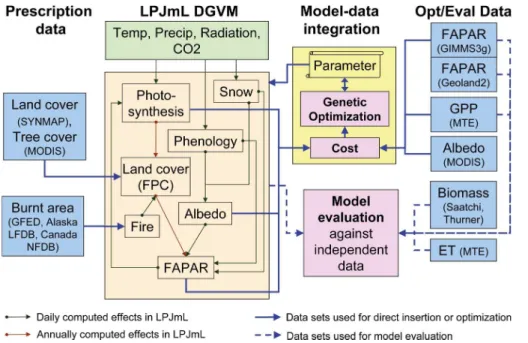
We developed a model-data integration approach for the LPJmL DGVM (LPJmL-MDI, Fig. 1). LPJmL-MDI allows to (1) directly insert land cover, tree cover and burnt area data sets in LPJmL for diagnostic model applications (Sec. 2.4.1), (2) to optimize LPJmL model parameters against datasets (here FAPAR, GPP, albedo; Sec. 2.4.2); and (3) to evaluate and benchmark LPJmL simulations against
observa-10
tions or observation-based data sets (Sec. 2.4.3). Like in a prognostic mode, LPJmL was driven by climate forcing data. Additionally, observed burnt areas were directly in-serted in LPJmL to consider observed fire dynamics in diagnostic model applications. For this, we directly replaced the simulated burnt area in the LPJmL-SPITFIRE fire module (Thonicke et al., 2010) by observed burnt areas using the approach of Lehsten
15
et al. (2008). Thus, the timing and location of fire spread is constrained by observations whereas fire effects on vegetation are still simulated by LPJmL-SPITFIRE. We further prescribed observed land cover and tree cover fractions to control for vegetation dy-namics in parameter optimization experiments. Observed FAPAR and albedo time se-ries as well as observation-based mean annual spatial patterns of GPP were used in
20
a joint cost function to optimize productivity, phenology, radiation, and albedo-related model parameters using a genetic optimization algorithm.
LPJmL was previously evaluated against site measurements of net carbon ecosys-tem exchange (Schaphoff et al., 2013; Sitch et al., 2003), atmospheric CO2 fractions (Sitch et al., 2003), soil moisture (Wagner et al., 2003), evapotranspiration and runoff
25
BGD
11, 10917–11025, 2014
Phenology controls and model-data
integration
M. Forkel et al.
Title Page
Abstract Introduction
Conclusions References
Tables Figures
◭ ◮
◭ ◮
Back Close
Full Screen / Esc
Printer-friendly Version Interactive Discussion
Discussion
P
a
per
|
Discus
sion
P
a
per
|
Discussion
P
a
per
|
Discussion
P
a
per
|
2013), GPP and evapotranspiration (ET) (Jung et al., 2011), tree cover (Townshend et al., 2011) and biomass (Saatchi et al., 2011; Thurner et al., 2014).
2.2 FAPAR and phenology in the LPJmL DGVM
2.2.1 FAPAR
FAPAR is defined as the ratio between the photosynthetic active radiation absorbed by
5
the green canopy (APAR) and the total incident photosynthetic active radiation (PAR). Thus, the total FAPAR of a grid cell is the sum of FAPAR that is distributed among the individual PFTs:
FAPARPFT=
APARPFT
PAR (1)
FAPARgridcell= PFT=n
X
PFT=1
FAPARPFT (2)
10
wherenis the number of established PFTs in a grid cell. The FAPAR of a PFT depends on the annual maximum foliar projective cover (FPC), on the daily snow coverage in the green canopy (Fsnow, gv), green-leaf albedo (βleaf) and the daily phenology status (Phen):
15
FAPARPFT=FPCPFT×(PhenPFT−(PhenPFT×Fsnow, gv, PFT))×(1−βleaf, PFT) (3)
Thus, the temporal dynamic of FAPAR in LPJmL is affected on an annual time step by changes in foliar projective cover (FPCPFT) and on daily time steps by changes in phenology (PhenPFT) and snow coverage in the green canopy (Fsnow, gv, PFT) (Fig. A1). 20
BGD
11, 10917–11025, 2014
Phenology controls and model-data
integration
M. Forkel et al.
Title Page
Abstract Introduction
Conclusions References
Tables Figures
◭ ◮
◭ ◮
Back Close
Full Screen / Esc
Printer-friendly Version Interactive Discussion
Discussion
P
a
per
|
Discus
sion
P
a
per
|
Discussion
P
a
per
|
Discussion
P
a
per
|
FPCPFTexpresses the land cover fraction of a PFT. It is the annual maximum frac-tional green canopy coverage of a PFT and is annually calculated from crown area (CA), population density (P) and LAI (Sitch et al., 2003):
FPCPFT=CAPFT×PPFT×(1−e
−kPFT×LAIPFT) (4)
5
The last term expresses the light extinction in the canopy which depends exponentially on LAI and the light extinction coefficientkof the Lambert–Beer law (Monsi and Saeki, 1953). The parameterkhad a constant value of 0.5 for all PFTs in the original LPJmL formulation (Sitch et al., 2003). We changedk to a PFT-dependent parameter because it varies for different plant species as seen from field observations (Bolstad and Gower,
10
1990; Kira et al., 1969; Monsi and Saeki, 1953). Crown area and leaf area index are calculated based on allocation rules and are depending on the annual biomass incre-ment (Sitch et al., 2003). Population density depends on establishincre-ment and mortality processes in LPJmL (Sitch et al., 2003).
2.2.2 Phenology
15
The daily phenology and green leaf status of a PFT (PhenPFT) in LPJmL expresses the fractional cover of green leaves (from 0=no leaves to 1=full leave cover). Thus, it represents the temporal dynamic of the canopy greenness. We explored two phenology models in this study: first, we were trying to optimize model parameters of the original phenology model in LPJmL (LPJmL-OP, Sitch et al., 2003, Appendix A1). Secondly,
20
we implemented a new phenology model based on the growing season index (GSI) concept (Jolly et al., 2005), hereinafter called LPJmL-GSI.
LPJmL-OP has three different routines for summergreen (i.e. temperature-driven de-ciduous), evergreen (no seasonal variation) and rain-green (i.e. water-driven decidu-ous) PFTs (details in Appendix A1). Obviously, LPJmL-OP misses important controls
25
BGD
11, 10917–11025, 2014
Phenology controls and model-data
integration
M. Forkel et al.
Title Page
Abstract Introduction
Conclusions References
Tables Figures
◭ ◮
◭ ◮
Back Close
Full Screen / Esc
Printer-friendly Version Interactive Discussion
Discussion
P
a
per
|
Discus
sion
P
a
per
|
Discussion
P
a
per
|
Discussion
P
a
per
|
is not controlled by environmental conditions but is defined based on fixed calendar dates.
Because of the obvious limitations of LPJmL-OP, we developed the alternative LPJmL-GSI phenology module. The growing season index (GSI) is an empirical phe-nology model that multiplies limiting effects of temperature, day length and vapour
pres-5
sure deficit (VPD) to a common phenology status (Jolly et al., 2005). We modified the GSI concept for the specific use in LPJmL (LPJmL-GSI). We defined the phenology status as a function of cold temperature, short-wave radiation and water availability. Ad-ditionally to the original GSI model, we added a heat stress limiting function because it has been suggested that vegetation greenness is limited by temperature-induced heat
10
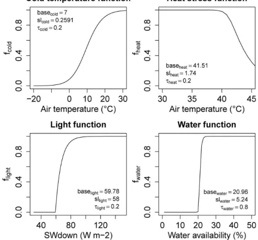
stress in several ecosystems (Bunn et al., 2007; Verstraeten et al., 2006) and has been demonstrated that heat stress reduces plant productivity also without additional water stress (Jiang and Huang, 2001; Van Peer et al., 2004; Poirier et al., 2012). Thus, the daily phenology status of a PFT is the product of the daily cold temperature (fcold, PFT), light (flight, PFT), water (fwater, PFT) and heat stress (fheat, PFT) limiting functions:
15
PhenPFT=fcold, PFT×flight, PFT×fwater, PFT×fheat, PFT (5)
Examples for the four functions are shown in Fig. 2.
The cold temperature limiting function at a daily time steptis defined as:
fcold, PFTt =ft−1 cold, PFT+
1
1+e−slcold, PFT×(T−basecold, PFT)−f
t−1 cold, PFT
×τcold, PFT (6)
20
where slcold, PFTand basecold, PFTare PFT-dependent slope and inflection point parame-ters of a logistic function based on daily air temperatureT (◦C). The parameterτcold, PFT is the change rate parameter based on the difference between the actual predicted lim-iting function value and the previous-day cold temperature limlim-iting function value. This
25
BGD
11, 10917–11025, 2014
Phenology controls and model-data
integration
M. Forkel et al.
Title Page
Abstract Introduction
Conclusions References
Tables Figures
◭ ◮
◭ ◮
Back Close
Full Screen / Esc
Printer-friendly Version Interactive Discussion
Discussion
P
a
per
|
Discus
sion
P
a
per
|
Discussion
P
a
per
|
Discussion
P
a
per
|
The light-limiting function was implemented accordingly:
flight, PFTt =ft−1 light, PFT+
1
1+e−sllight, PFT×(SW−baselight, PFT) −f
t−1 light, PFT
×τlight, PFT (7)
where sllight, PFT and baselight, PFT are the PFT-dependent slope and inflection point parameters of a logistic function based on daily shortwave downward radiation SW
5
(W m−2). The parameterτlight, PFTis the temporal change rate for the light-limiting func-tion.
The water-limiting functionfwater, PFTdepends on the daily water availabilityW (%) in LPJmL:
fwater, PFTt =ft−1 water, PFT+
1
1+e−slwater, PFT×(W−basewater, PFT)−f
t−1 water, PFT
×τwater, PFT (8)
10
where slwater, PFT and basewater, PFT are the PFT-dependent slope and inflection point parameters of a logistic function based on daily water availability.W is a ratio between water supply from soil moisture and atmospheric water demand (Appendix A.2) (Gerten et al., 2004). The parameterτwater, PFTis the temporal change rate for the water-limiting
15
function.
The heat-stress limiting function is defined as the cold-temperature limiting function based on daily air temperature but with a negative slope parameter:
fheat, PFTt =ft−1 heat, PFT+
1
1+eslheat, PFT×(T−baseheat, PFT) −ft−1
heat, PFT
×τheat, PFT (9)
20
where slheat, PFT and baseheat, PFT are the PFT-dependent slope and inflection point parameters of a logistic function based onT. The parameterτheat, PFT is the temporal change rate for the heat limiting function.
Besides the additional use of the heat stress limiting function, LPJmL-GSI has im-portant differences to the original GSI phenology model (Jolly et al., 2005) We made
BGD
11, 10917–11025, 2014
Phenology controls and model-data
integration
M. Forkel et al.
Title Page
Abstract Introduction
Conclusions References
Tables Figures
◭ ◮
◭ ◮
Back Close
Full Screen / Esc
Printer-friendly Version Interactive Discussion
Discussion
P
a
per
|
Discus
sion
P
a
per
|
Discussion
P
a
per
|
Discussion
P
a
per
|
the water limiting function dependent on water availability. VPD has been used instead in the original GSI phenology model. Nevertheless, it has been shown that phenology is more driven by soil moisture and plant available water than by atmospheric water de-mand especially in Mediterranean and grassland ecosystems (Archibald and Scholes, 2007; Kramer et al., 2000; Liu et al., 2013; Yuan et al., 2007) and that GSI performed
5
better when using a soil moisture limiting function instead of the VPD limiting func-tion (Migliavacca et al., 2011). With the implementafunc-tion of the water limiting funcfunc-tion in LPJmL-GSI, phenology depends not only on atmospheric water demand as in the original GSI model but also on water supply from soil moisture. Additionally, the soil moisture can be modulated through seasonal freezing and thawing in permafrost soils
10
according to the permafrost routines in LPJmL (Schaphoffet al., 2013). Another im-portant difference to the original GSI phenology model is the use of logistic functions instead of stepwise linear functions with fixed thresholds because smooth functions are generally easier to optimize than functions with abrupt thresholds and potentially better represent biological processes. A moving average of 21 days has been used in the
15
original GSI model to create smooth phenological cycles and to avoid abrupt phenol-ogy changes because of daily weather variability (Jolly et al., 2005). It has been shown that PFT- and limiting function-dependent time averaging parameters are needed in-stead of one single time averaging parameter (Stöckli et al., 2011). We implemented change rate parametersτcold,τlight,τwater andτheat that are PFT- and limiting function-20
dependent instead of moving average window lengths because LPJmL as a prognostic model cannot use a running window time averaging approach.
2.3 Data sets
2.3.1 Data sets for parameter optimization: FAPAR, albedo and GPP
We used FAPAR, albedo and GPP data sets to optimize phenology, FAPAR,
productiv-25
BGD
11, 10917–11025, 2014
Phenology controls and model-data
integration
M. Forkel et al.
Title Page
Abstract Introduction
Conclusions References
Tables Figures
◭ ◮
◭ ◮
Back Close
Full Screen / Esc
Printer-friendly Version Interactive Discussion
Discussion
P
a
per
|
Discus
sion
P
a
per
|
Discussion
P
a
per
|
Discussion
P
a
per
|
time scales. Two recently developed datasets provide 30 year time series of FAPAR. The Geoland2 BioPar (GEOV1) FAPAR dataset (Baret et al., 2013) (hereinafter called GL2 FAPAR) and the GIMMS3g FAPAR (Zhu et al., 2013) datasets were used in this study.
GL2 FAPAR is defined as the black-sky green canopy FAPAR at 10:15 solar time
5
and has been produced based on SPOT VGT (1999–2012) and AVHRR (1981–2000) (Baret et al., 2013). The GL2 FAPAR dataset has a temporal resolution of 10 days and a spatial resolution of 0.05◦ for the AVHRR-period and of 1/112◦ for the SPOT VGT period. GIMMS3g FAPAR corresponds to black-sky FAPAR at 10:35 solar time and has been produced based on the GIMMS3g NDVI dataset (Zhu et al., 2013). GIMMS3g
10
FAPAR has a 15 day temporal resolution and a 1/12◦ spatial resolution and covers July 1981 to December 2011. We excluded in both FAPAR datasets observations that were flagged as contaminated by snow, aerosols or clouds. Additionally, we excluded FAPAR observations for months with temperatures<0◦C to exclude potential remain-ing distortions of snow cover. Both datasets were aggregated to a 0.5◦ spatial and
15
monthly temporal resolution to be comparable with LPJmL simulations. We found that the GL2 AVHRR and GL2 VGT FAPAR datasets have not been well harmonized (Ap-pendix B1). Thus, we did not use the combined GL2 VGT and AVHRR FAPAR dataset for parameter optimization and for analyses of inter-annual variability and trends but only for analyses and evaluations of mean seasonal cycles and spatial patterns of
20
FAPAR. The GIMMS3g FAPAR dataset has no uncertainty estimates. Uncertainty es-timates are necessary in multiple data stream parameter optimization to weight single data streams in the total cost function. As a workaround we estimated the uncertainty based on monthly-varying quantile regressions to the 0.95 quantile between FAPAR and the FAPAR uncertainty in the GL2 VGT dataset. We applied the fitted regressions
25
BGD
11, 10917–11025, 2014
Phenology controls and model-data
integration
M. Forkel et al.
Title Page
Abstract Introduction
Conclusions References
Tables Figures
◭ ◮
◭ ◮
Back Close
Full Screen / Esc
Printer-friendly Version Interactive Discussion
Discussion
P
a
per
|
Discus
sion
P
a
per
|
Discussion
P
a
per
|
Discussion
P
a
per
|
We used monthly shortwave white-sky albedo time series ranging from 2000 to 2010 from the MODIS C5 dataset (Lucht et al., 2000; Schaaf et al., 2002) to constrain veg-etation albedo parameters. Albedo observations in months with<5◦C air temperature and above an albedo of 0.3 were excluded from optimization because we are optimiz-ing only vegetation-related albedo parameters. High albedo values at low temperatures
5
are probably affected by changing snow regimes which is not within our focus of model development and optimization. Thus we are only optimizing growing season albedo.
We used mean annual total GPP patterns from the data-oriented MTE (model tree ensemble) GPP estimate (Jung et al., 2011). This GPP estimate uses FLUXNET eddy covariance observations together with satellite observations and climate data to
up-10
scale GPP using a machine learning approach (Jung et al., 2011). This dataset is not an observation but a result of an empirical model. Nevertheless, evaluation and cross-validation analyses have shown that this dataset well represents the mean annual spa-tial patterns and mean seasonal cycles of GPP whereas it has a poor performance in representing temporal GPP anomalies (trends and extremes) (Jung et al., 2011). Thus,
15
we are only using the mean annual total GPP from this dataset for parameter optimiza-tion to constrain LPJmL within small biases of mean annual GPP. We used the mean seasonal cycle from the MTE GPP product as an independent benchmark for model evaluation.
2.3.2 Data sets for the prescription of land cover, tree cover and burnt area 20
The FAPAR, albedo and GPP data sets do not presumably contain enough informa-tion to constrain all processes that control FAPAR dynamics. Especially, processes like establishment, mortality, competition between PFTs, allocation and disturbances con-trol FPC and thus FAPAR. The optimization of parameters of these processes against appropriate data streams is not feasible within this study. Thus, we directly prescribed
25
BGD
11, 10917–11025, 2014
Phenology controls and model-data
integration
M. Forkel et al.
Title Page
Abstract Introduction
Conclusions References
Tables Figures
◭ ◮
◭ ◮
Back Close
Full Screen / Esc
Printer-friendly Version Interactive Discussion
Discussion
P
a
per
|
Discus
sion
P
a
per
|
Discussion
P
a
per
|
Discussion
P
a
per
|
To prescribe land and tree cover in LPJmL, we combined several datasets to create observation-based maps of FPC (Appendix C2). Land cover maps from remote sensing products are not directly comparable with PFTs in global vegetation models due to differences in classification systems (Jung et al., 2006; Poulter et al., 2011a). PFTs in LPJmL are defined according to biome (tropical, temperate or boreal), leaf type (needle
5
leaved, broadleaved) and phenology type (summergreen, evergreen, rain green). We extracted the biome information from the Köppen–Geiger climate classification (Kottek et al., 2006) whereas leaf type and phenology were extracted from the SYNMAP land cover map (Jung et al., 2006). FPC was derived from MODIS tree cover (Townshend et al., 2011). Because LPJmL so far classified herbaceous vegetation according to their
10
photosynthetic pathway (i.e. C3, temperate herbaceous and C4, tropical herbaceous), we further sub-divided herbaceous PFTs according to biome and introduced a polar herbaceous PFT (PoH) based on the existing temperate herbaceous PFT (TeH) to differentiate tundra from temperate grasslands.
Burnt area data was prescribed directly in LPJmL by combining three data sets, the
15
Global Fire Emissions Database (GFED) burnt area dataset (Giglio et al., 2010), the Alaska Large Fire Database (ALFDB) (Frames, 2012; Kasischke et al., 2002) and the Canadian National Fire Database (CNFDB) (CFS, 2010; Stocks et al., 2002). GFED provides monthly burnt area estimates in 0.5◦resolution from 1996 to 2011. Burnt ar-eas from the Alaska (ALFDB) and Canada (CNFDB) fire databases were used to extent
20
burnt area time-series before 1996 for boreal North America. Fire perimeter observa-tions from 1979 to 1996 from ALFDB and CNFDB were aggregated to 0.5◦ gridded monthly burnt area time series. Observations before 1979 were excluded because fires were not reported for all provinces in Canada. Although the CNFDB contains only fire perimeters>200 ha, in both databases some fires are missing due to different mapping
25
BGD
11, 10917–11025, 2014
Phenology controls and model-data
integration
M. Forkel et al.
Title Page
Abstract Introduction
Conclusions References
Tables Figures
◭ ◮
◭ ◮
Back Close
Full Screen / Esc
Printer-friendly Version Interactive Discussion
Discussion
P
a
per
|
Discus
sion
P
a
per
|
Discussion
P
a
per
|
Discussion
P
a
per
|
as well. Otherwise biomass would be overestimated at the beginning of the transient model run. For this purpose, we created artificial burnt area time series for the periods 1901–1978 (North America) and 1901–1995 (rest of the world). Observed annual total burnt areas from the periods 1979–2011 (North America) and 1996–2011 (rest of the world) were resampled according to temperature and precipitation conditions and
as-5
signed to the pre-data period in order to include fire regimes that agree with observed fire regimes in the spin-up of LPJmL. This approach assumes that fire regimes in the pre-data period were not different than in the observation period.
2.3.3 Data sets for model evaluation
LPJmL was evaluated against data sets that are independent from the optimization
10
and prescription data sets and against independent temporal or spatial scales of the optimization and prescription data sets. We compared LPJmL against mean annual patterns and mean seasonal cycles of ET from the MTE estimate (Jung et al., 2011). Further, we evaluated model results against spatial patterns of biomass. Ecosystem biomass estimates were taken from satellite-derived forest biomass maps for the
trop-15
ics (Saatchi et al., 2011) and for the temperate and boreal forests (Thurner et al., 2014) including an estimation of herbaceous biomass. Additionally, we evaluated LPJmL against independent temporal and spatial scales of the integration data (mean sea-sonal cycle of GPP, tree cover, inter-annual variability and trends of FAPAR). We were using tree cover from MODIS to evaluate LPJmL model runs with dynamic vegetation.
20
2.3.4 Climate forcing data and model spin-up
LPJmL was driven by observed monthly temperature and precipitation data from the CRU TS3.1 dataset ranging from 1901 to 2011 (Harris et al., 2013) as well as by monthly shortwave downward radiation and long wave net radiation re-analysis data from ERA-Interim (Dee et al., 2011).
BGD
11, 10917–11025, 2014
Phenology controls and model-data
integration
M. Forkel et al.
Title Page
Abstract Introduction
Conclusions References
Tables Figures
◭ ◮
◭ ◮
Back Close
Full Screen / Esc
Printer-friendly Version Interactive Discussion
Discussion
P
a
per
|
Discus
sion
P
a
per
|
Discussion
P
a
per
|
Discussion
P
a
per
|
LPJmL needs a model spin-up to establish PFTs and to bring vegetation and soil carbon pools into equilibrium. The spin-up was performed according to the standard LPJmL modeling protocol (Schaphoffet al., 2013; Thonicke et al., 2010): LPJmL was run for 5000 years by repeating the climate data from 1900–1930. After the spin-up model run, the transient model run was restarted from the spin-up conditions in 1901
5
and LPJmL was run for the period 1901–2011. Model results were analyzed for the observation period (1982–2011).
For model optimization experiments we used a different spin-up scheme because the spin-up is computational time demanding and many model runs are needed during optimization experiments. As in the standard modeling protocol, we firstly spin-up the
10
model for 5000 years by repeating the climate from 1901–1930. Secondly, a transient model run was restarted from the spin-up conditions in 1901 and was performed for the period 1901–1979. Thirdly, each optimization experiment was restarted from the con-ditions in 1979 and a second spin-up for 100 years by recycling the climate from 1979 to 1988 was performed. The transient model run was restarted from the conditions of
15
the second spin-up and simulated for the period 1979–2011. This second spin-up is needed to bring the vegetation into a new equilibrium which can be caused by a new parameter combination during optimization. From visual analyses of model results, we found that a spin-up time of 100 years for the second spin-up was enough to eliminate trends in FAPAR and GPP that resulted from other equilibrium conditions.
20
2.4 Model-data integration
2.4.1 Prescription of land and tree cover
Land cover is expressed as FPC in LPJmL. We used the observation-based FPC dataset to prescribe land and tree cover in LPJmL (Sec. 2.3.2, Appendix C1). The presence of a PFT in a grid cell depends on establishment and mortality in LPJmL
25
BGD
11, 10917–11025, 2014
Phenology controls and model-data
integration
M. Forkel et al.
Title Page
Abstract Introduction
Conclusions References
Tables Figures
◭ ◮
◭ ◮
Back Close
Full Screen / Esc
Printer-friendly Version Interactive Discussion
Discussion
P
a
per
|
Discus
sion
P
a
per
|
Discussion
P
a
per
|
Discussion
P
a
per
|
in a grid cell if the climate is no longer suitable for the PFT. Additionally, mortality oc-curs because of heat stress, low productivity, competition among PFTs for light, and because of fire disturbance (Sitch et al., 2003; Thonicke et al., 2010).
FPC is the major variable that contributes to inter-annual variability of FAPAR in LPJmL despite the daily phenological status. Thus fixing FPC to the observed value
5
is not a desired solution to prescribe land cover in LPJmL. Fixing FPC would neglect mortality effects on land cover but would also permit the simulation of post-fire suc-cession trajectories. Consequently, we prescribed land cover in LPJmL using a hy-brid diagnostic-dynamic approach. In this approach we prescribed the annual maxi-mum FPC in LPJmL similar to previous approaches (Poulter et al., 2011b). Firstly, we
10
switched offthe effects of bioclimatic limits on establishment and mortality. Only these PFTs were allowed to establish in a grid cell that occurred in the observed land-cover data set. Vegetation growth depends on the annual biomass increment and allocation rules in LPJmL. This leads to an extension of FPC of each PFT. We limited a further expansion of FPC if the simulated FPC values equals the observed FPC (prescribed
15
maximum FPC). In this case, no new individuals are established and the population densityP of a PFT is corrected in order to fit the observed FPC (FPCobs):
PPFT,corr=PPFT×FPCPFT−(FPCPFT−FPCobs, PFT) (10)
The biomass of the individuals that need to be killed in order to match the corrected
20
population densityPPFT,corr is transferred to the litter pools. The simulated FPC can be lower than the observed FPC because the PFT is still growing or because the FPC was reduced due to fire, heat stress or low productivity. For herbaceous PFTs we only reduced the FPC if the observed total fractional vegetation cover in a grid cell was exceeded. This allows herbaceous PFTs to replace tree PFTs if the FPC of trees is
25
BGD
11, 10917–11025, 2014
Phenology controls and model-data
integration
M. Forkel et al.
Title Page
Abstract Introduction
Conclusions References
Tables Figures
◭ ◮
◭ ◮
Back Close
Full Screen / Esc
Printer-friendly Version Interactive Discussion
Discussion
P
a
per
|
Discus
sion
P
a
per
|
Discussion
P
a
per
|
Discussion
P
a
per
|
2.4.2 Parameter optimization
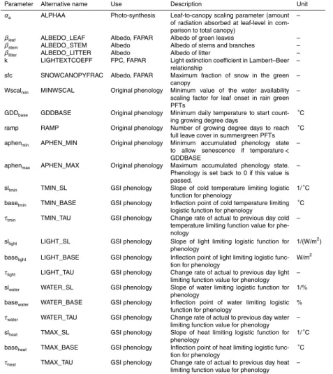
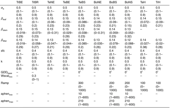
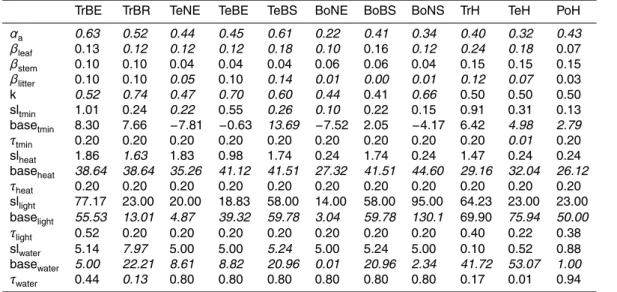
Photosynthesis, albedo, FAPAR and phenology-related model parameters of LPJmL were optimized against observed FAPAR and albedo satellite observations and data-oriented estimates of GPP. A description of all parameters including parameter values is given in Appendix D1. The parameterαais the most important parameter in LPJmL 5
for photosynthesis (Zaehle et al., 2005). This parameter accounts for the amount of ra-diation that is absorbed at leaf level in comparison to the total canopy. Thus, this param-eter is a replacement for a more enhanced model formulation for canopy structure and leaf clumping. We used this parameter to adjust biases in GPP. The PFT-dependent leaf, stem and litter albedo parameters (βleaf,βstem andβlitter) are mostly sensitive for 10
model simulations of albedo. The parameterβleaf affects additionally the maximum FA-PAR of a PFT. The light extinction coefficientk controls the FPC of a PFT and thus affects mainly land cover, maximum FAPAR and the available radiation for photosyn-thesis. All other parameters that were considered in optimization experiments are the parameters of the LPJmL-OP and LPJmL-GSI phenology modules. These parameters
15
contribute mainly to seasonal variations in FAPAR. Some parameters were excluded from optimization experiments that were identified as insensitive to GPP and FAPAR simulations in PFTs. The temporal change rate parametersτtmin,τlight,τheat andτwater are insensitive in most PFTs because of the monthly temporal resolution of the used climate forcing data.
20
The optimization of model parameters was performed by minimizing a cost func-tion between model simulafunc-tions and observafunc-tions using a combined genetic and gradient-based optimization algorithm (GENOUD, genetic optimization using deriva-tives, Mebane and Sekhon, 2011, see Appendix D2 for details). The cost functionJ of LPJmL for a single model grid cell (gc) depends on the scaled model parameter vector
25
d (d=parameter value/prior parameter value) and is the sum of square error (SSE)
BGD
11, 10917–11025, 2014
Phenology controls and model-data
integration
M. Forkel et al.
Title Page
Abstract Introduction
Conclusions References
Tables Figures
◭ ◮
◭ ◮
Back Close
Full Screen / Esc
Printer-friendly Version Interactive Discussion
Discussion
P
a
per
|
Discus
sion
P
a
per
|
Discussion
P
a
per
|
Discussion
P
a
per
|
(nobs) for each data stream (DS):
J(d)gc=
DS=n
X
DS=1
SSEDS(d) nobsDS
(11)
The SSE for a single data stream is calculated from the LPJmL simulation of this data stream (xLPJmL) and the corresponding observed values (xobs) weighted by the uncer-5
tainty of the observations (xobsunc) for each time stept:
SSE(d)=
t=n
X
t=1
(xLPJmL,t(d×p0)−xobs,t)
2
xobsunc,2 t (12)
wherep0 are LPJmL prior parameters. That means the minimization of the cost func-tionJ is based on scalars of LPJmL parameters relative to the prior parameter values.
10
Different model optimization experiments were performed for individual grid cell and for multiple grid cells of the same PFT for LPJmL-OP as well as for LPJmL-GSI (Ta-ble 1). In the grid cell-based optimization experiments model parameters of the es-tablished target tree PFT and the eses-tablished herbaceous PFT were optimized at the same time. The purpose of grid cell-level optimization experiments was to explore the
15
variability of parameters within different regions and PFTs. In the PFT-level optimization experiments the cost of LPJmL was calculated as the sum of the cost for each grid cell weighted by the grid cell area A:
J(d)PFT=
Pgc=n
gc=1J(d)gc×Agc Pn
gc=1Agc
(13)
20
BGD
11, 10917–11025, 2014
Phenology controls and model-data
integration
M. Forkel et al.
Title Page
Abstract Introduction
Conclusions References
Tables Figures
◭ ◮
◭ ◮
Back Close
Full Screen / Esc
Printer-friendly Version Interactive Discussion
Discussion
P
a
per
|
Discus
sion
P
a
per
|
Discussion
P
a
per
|
Discussion
P
a
per
|
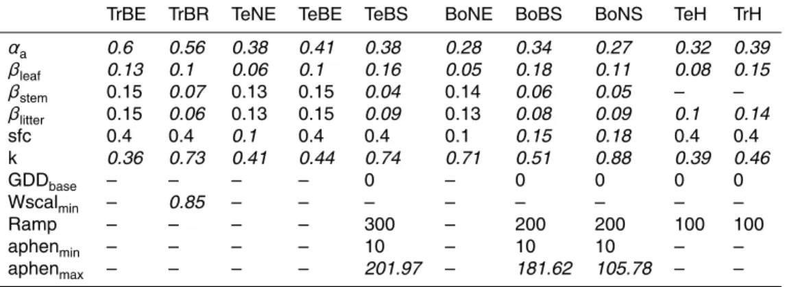
PFT. The purpose of PFT-level optimization experiments is to derive optimized param-eter sets that can be used for one PFT in global model runs.
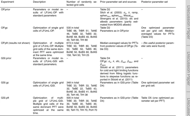
For grid cell as well PFT-level optimization experiments, we only used grid cells that are vegetated, dominated by one PFT and that are only marginally affected from agri-cultural use or fire disturbances. These grid cells are called candidate grid cells in
5
the following. We randomly selected grid cells from the set of candidate grid cells to perform grid cell- or PFT-level optimization experiments. Table 1 gives an overview of all optimization experiments for LPJmL-OP and LPJmL-GSI with the number of used grid cells. Grid cells that were selected for optimization experiments are also shown in Fig. 3. The PFT-level optimization of LPJmL-OP (OP.pft) did not result in plausible
10
posterior parameter sets because of structural limitations of the LPJmL-OP phenol-ogy model for herbaceous PFTs (i.e. no water effects, calendar day as end of growing season), raingreen PFT (i.e. binary phenology) and evergreen PFTs (i.e. constant phe-nology) and was therefore excluded from further analysis.
Parameter sensitivities and uncertainties were explored by analyzing the maximum
15
likelihood and the posterior range of each parameter as derived from all parameter sets from the genetic optimization algorithm (Appendix D3).
2.4.3 Model evaluation and time series analysis
Global model runs of LPJmL were performed in order to evaluate model results against the integration data, against independent metrics of the integration data and against
20
independent data streams. We evaluated results from LPJmL-OP with standard pa-rameters (LPJmL-OP-prior), from LPJmL-OP with optimized productivity, albedo and FAPAR parameters from grid-cell level optimization experiments (LPJmL-OP-gc) and from LPJmL-GSI with optimized parameters from PFT-level optimization experiments (Table 2). We did not use optimized phenology parameters in the LPJmL-OP-gc model
25
BGD
11, 10917–11025, 2014
Phenology controls and model-data
integration
M. Forkel et al.
Title Page
Abstract Introduction
Conclusions References
Tables Figures
◭ ◮
◭ ◮
Back Close
Full Screen / Esc
Printer-friendly Version Interactive Discussion
Discussion
P
a
per
|
Discus
sion
P
a
per
|
Discussion
P
a
per
|
Discussion
P
a
per
|
We aggregated monthly FAPAR time series to mean annual FAPAR to evaluate inter-annual variability and trends. Mean inter-annual FAPAR time series were averaged from all monthly values with mean monthly air temperatures>0◦C to exclude potential remain-ing effects of snow in the observed FAPAR time series. Trends in mean annual FAPAR time series and trend breakpoints were computed using the “greenbrown” package for
5
R software (Forkel et al., 2013). In this implementation, trends are computed by fitting piece-wise linear trends to the annual FAPAR time series using ordinary least squares regression. The significance of trends was computed using the Mann–Kendall trend test (Mann, 1945).
3 Results and discussions
10
3.1 Parameter optimization
3.1.1 Performance of phenology models
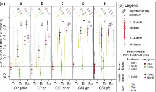
The newly developed LPJmL-GSI phenology model resulted in significantly higher cor-relations with monthly GIMMS3g FAPAR than LPJmL-OP in all PFTs except in the tropical broadleaved evergreen (TrBE) and boreal broadleaved summergreen (BoBS)
15
PFTs (Fig. 4). LPJmL-OP with prior parameters had high correlations with monthly GIMMS3g FAPAR in broad-leaved summergreen PFTs (TeBS medianr =0.87, BoBS medianr=0.92) PFTs and medium correlations in boreal needle-leaved PFTs (BoNE median r=0.53, BoNS median r=0.6). In all other PFTs, LPJmL-OP had low cor-relations with monthly GIMMS3g FAPAR. The correlation against monthly GIMMS3g
20
FAPAR did not significantly improve in all PFTs after grid cell-level optimization exper-iments of LPJmL-OP (Fig. 4). The use of the newly developed LPJmL-GSI phenology model already significantly improved the correlation with monthly GIMMS3g FAPAR in all PFTs except in the temperate herbaceous (TeH) and BoBS PFTs. LPJmL-GSI had significantly higher correlations with monthly GIMMS3g FAPAR after grid cell-level
BGD
11, 10917–11025, 2014
Phenology controls and model-data
integration
M. Forkel et al.
Title Page
Abstract Introduction
Conclusions References
Tables Figures
◭ ◮
◭ ◮
Back Close
Full Screen / Esc
Printer-friendly Version Interactive Discussion
Discussion
P
a
per
|
Discus
sion
P
a
per
|
Discussion
P
a
per
|
Discussion
P
a
per
|
mization experiments in the TrBR, TeNE, TeBS, TeH, BoBS and BoNS PFTs. After PFT-level optimization experiments, LPJmL-GSI had median correlation coefficients>0.5 in all PFTs except in broadleaved evergreen PFTs (TrBE, TeBE). These results prove that the rain-green, evergreen and herbaceous phenology schemes of LPJmL-OP were not able to reproduce temporal FAPAR dynamics despite the attempt of parameter
5
optimization and that LPJmL-GSI can reproduce seasonal FAPAR dynamics in most PFTs.
The low correlations coefficients between LPJmL-GSI and GIMMS3g FAPAR af-ter optimization experiments in broadleaved evergreen PFTs (TrBE, TeBE) might be caused by the specific properties of the FAPAR dataset in these PFTs. GIMMS3g
FA-10
PAR does not have a clear seasonal cycle but a high short-term variability in tropical broadleaved evergreen forests. These regions are often covered by clouds that inhibit continuous optical satellite observations. The high short-term variability results ulti-mately in low correlation coefficients between both LPJmL versions (LPJmL-OP and LPJmL-GSI) and GIMMS3g FAPAR time series. Besides climatic factors, phenology
15
in tropical forests is more driven by leaf age (Caldararu et al., 2012, 2014) and nutri-ent availability (Wright, 1996). These affects are neither considered in the original GSI phenology model (Jolly et al., 2005; Stöckli et al., 2011) nor in the LPJmL-GSI phenol-ogy model. In temperate broadleaved evergreen forests, the GIMMS3g FAPAR dataset might have a wrong seasonality. In these regions, the mean seasonal FAPAR cycles
20
from the GIMMS3g and GL2 VGT FAPAR datasets are anti-correlated and FAPAR from LPJmL-GSI agrees better with the GL2 VGT dataset. Because of these reasons, we did not expect to improve seasonal FAPAR dynamics in broadleaved evergreen forests with the current model-data integration setup.
All optimization experiments of LPJmL-OP and LPJmL-GSI resulted in a
signifi-25
BGD
11, 10917–11025, 2014
Phenology controls and model-data
integration
M. Forkel et al.
Title Page
Abstract Introduction
Conclusions References
Tables Figures
◭ ◮
◭ ◮
Back Close
Full Screen / Esc
Printer-friendly Version Interactive Discussion
Discussion
P
a
per
|
Discus
sion
P
a
per
|
Discussion
P
a
per
|
Discussion
P
a
per
|
boreal needle-leaved summergreen PFTs. The reduction of the overall cost was in all model optimization experiments usually associated with a significant reduction of the annual GPP bias (Fig. D3). LPJmL-OP with prior parameters underestimated mean an-nual GPP in the tropical broad-leaved evergreen PFT and overestimated mean anan-nual GPP in all other PFTs. Grid cell-level optimization experiments of LPJmL-OP resulted in
5
a significant reduction of the GPP bias in all PFTs except in the polar herbaceous PFT (PoH). We were not able to remove the GPP bias and to reduce the cost of LPJmL-OP and of LPJmL-GSI in the PoH PFT (i.e. tundra) in optimization experiments because of inconsistencies between the FAPAR and GPP datasets or in the LPJmL formulation. LPJmL was not able to sustain the relatively high peak FAPAR in Tundra regions as
10
seen in the GIMMS3g dataset given the low mean annual GPP of the MTE dataset (Appendix D4). These inconsistencies might be related to higher uncertainties of the GPP and FAPAR datasets in tundra regions where the MTE GPP dataset is not cov-ered by many eddy covariance measurement sites, and where satellite-based FAPAR observations are affected from high sun zenith angles (Tao et al., 2009; Walter and
15
Shea et al., 1998). On the other hand, dominant tundra plant communities like mosses and lichen are not represented in LPJmL (Appendix D4). All model optimizations exper-iments kept growing season albedo within reasonable ranges in comparison to MODIS albedo (Fig. D4). These results demonstrate an improved performance of optimized model parameter sets over prior model parameter sets and of GSI over
LPJmL-20
OP regarding a cost that is defined based on 30 years of monthly FAPAR, mean annual GPP and 10 years of monthly vegetation albedo.
3.1.2 Parameter sensitivities and uncertainties
The uncertainty of productivity and albedo-related parameters was reduced after optimization of LPJmL-GSI in most PFTs while the reduction of the uncertainty of
25
BGD
11, 10917–11025, 2014
Phenology controls and model-data
integration
M. Forkel et al.
Title Page
Abstract Introduction
Conclusions References
Tables Figures
◭ ◮
◭ ◮
Back Close
Full Screen / Esc
Printer-friendly Version Interactive Discussion
Discussion
P
a
per
|
Discus
sion
P
a
per
|
Discussion
P
a
per
|
Discussion
P
a
per
|
The parameter αa (absorption of light at leaf level in relation to canopy level) was sensitive within a narrow parameter range for all PFTs. The posterior αa parameter range was smaller than the uniform prior range in all PFTs. In all optimization exper-iments we found for the parameter αa a gradient from high values in tropical to low values in boreal PFTs (Fig. D5). This pattern reflects the initial overestimation of mean
5
annual GPP in temperate and boreal PFTs and underestimation of GPP in tropical re-gions with the prior parameter set of LPJmL-OP. Thus, the lowαa parameter values accounts for nitrogen limitation effects on productivity in boreal forests (Vitousek and Howarth, 1991) that are currently not considered in LPJmL. A future implementation of nitrogen limitation processes in LPJmL requires a re-optimization of theαaparameter.
10
The leaf albedo parameter βleaf was sensitive in all PFTs and the posterior βleaf parameter range was smaller than the prior parameter range in evergreen PFTs. In these evergreen PFTs theβleaf parameter was well constrained because albedo satel-lite observations are less affected by variations in background albedo (soil, snow) than in deciduous PFTs. In all other PFTs the βleaf posterior parameter range was equal 15
the prior parameter range or the optimized parameter value was close to a boundary of the prior parameter range. This result indicates that the albedo routines in LPJmL should consider variations in background albedo caused by changes in soil properties, soil moisture or snow conditions in order to accurately reproduce satellite-observed albedo time series (see supplementary discussion in Appendix D5). Nevertheless, the
20
optimization of the leaf albedo parameter βleaf resulted in values that differed espe-cially between broadleaved and needle-leaved evergreen PFTs as well as herbaceous PFTs (Figs. 5 and D6). Low leaf albedo parameters in needle-leaved evergreen PFTs (TeNE and BoNE) and high leaf albedo parameters in broad-leaved summergreen and herbaceous PFTs agree well with the patterns reported by Cescatti et al. (2012).
25
BGD
11, 10917–11025, 2014
Phenology controls and model-data
integration
M. Forkel et al.
Title Page
Abstract Introduction
Conclusions References
Tables Figures
◭ ◮
◭ ◮
Back Close
Full Screen / Esc
Printer-friendly Version Interactive Discussion
Discussion
P
a
per
|
Discus
sion
P
a
per
|
Discussion
P
a
per
|
Discussion
P
a
per
|
Thus, this parameter cannot be well constrained for tree PFTs in the current optimiza-tion setup because the maximum FPC of trees was prescribed from the land and tree cover dataset. On the other hand, the maximum FPC of herbaceous PFTs was not prescribed from observations which resulted in narrow k posterior parameter ranges for herbaceous PFTs. The parameterk was optimized towards a very high value in
5
the BoNS PFT (k=0.7) due to high tree mortality rates after low-productivity years (Appendix D5). This parameter would result in a overestimated PFT coverage in model runs with dynamic vegetation. Thus, we performed a second optimization experiment for this PFT (blue in Fig. 5) where kBoNS was limited to 0.65. This optimization ex-periment resulted in similar posterior values for the other parameters. Although thek 10
parameter was well constrained for the TrH, TeH and PoH PFTs, these parameters cannot be used in the final parameter set of LPJmL-GSI. In dynamic vegetation model runs, the relatively lowkparameter values for the TrH and TeH PFTs and relatively high values for the PoH PFT would result in an underestimation of herbaceous coverage in temperate and tropical climates and an overestimation of herbaceous coverage in
bo-15
real and polar climates, respectively. Therefore, we performed three more optimization experiments for herbaceous PFTs where we fixedk at 0.5 (blue in Fig. 5). These opti-mization experiments resulted in similarαaparameters but different albedo parameters and phenology parameters in order to compensate for biases in FAPAR and albedo that were introduced by the fixedkparameter. Thus, the high spatial variability and the
20
large uncertainty of the light extinction coefficientk require re-addressing this param-eter in a model optimization setup with dynamic vegetation using tree and vegetation cover data or perhaps a replacement by a better representation of canopy architecture and radiative transfer.
The sensitivity and posterior uncertainty of phenology-related model parameters
de-25
BGD
11, 10917–11025, 2014
Phenology controls and model-data
integration
M. Forkel et al.
Title Page
Abstract Introduction
Conclusions References
Tables Figures
◭ ◮
◭ ◮
Back Close
Full Screen / Esc
Printer-friendly Version Interactive Discussion
Discussion
P
a
per
|
Discus
sion
P
a
per
|
Discussion
P
a
per
|
Discussion
P
a
per
|
effect of heat stress on phenology was sensitive in TrBR, TrH, TeH, BoNE and BoNS PFTs while in other PFTs this parameter was only sensitive towards the boundaries of the prior parameter range. Nevertheless, the posterior parameter range was only smaller than the prior parameter range in TrBR and TrH PFTs. The parameter baselight was sensitive in temperate and boreal PFTs. In tropical PFTs this parameter is only
5
sensitive above a certain threshold (i.e. 60 W m−2 for TrBE and 100 W m−2 for TrBR). The parameter basewater was sensitive in all PFTs. The posterior parameter range of this parameter was smaller in all PFTs except in TeBS, BoNE, BoBS and BoNS PFTs. Although, the parameter basewaterhad a large variability among PFTs, it was generally optimized towards higher values in PFTs that are presumably water-controlled (TrBR,
10
TeBS, TrH, TeH) and optimized towards lower values in PFTs that are presumably less water controlled (TrBE, TeNE, BoNE, BoNS, PoH). This result indicates that FAPAR of water-controlled PFTs reacts already to small decreases in water availability whereas other PFTs react only to strong decreases in water availability. As the basewater param-eter was the only phenology paramparam-eter which was sensitive in all PFTs, indicates that
15
water availability is the only phenological control that acts in all PFTs.
3.2 Global model evaluation
3.2.1 GPP, ET, biomass and tree cover
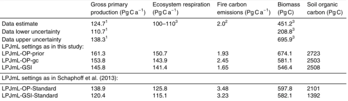
LPJmL-GSI and LPJmL-OP-gc with optimized parameters better represented global patterns of gross primary production, biomass and tree cover than LPJmL with
origi-20
nal phenology and prior parameters (LPJmL-OP-prior) (Fig. 6). LPJmL-OP-prior over-estimated mean annual GPP and biomass in most polar, boreal and temperate re-gions. LPJmL-OP-prior underestimated mean annual GPP but overestimated mean annual biomass in tropical regions around the Equator. These biases were reduced in LPJmL-OP-gc and LPJmL-GSI. LPJmL generally overestimated GPP also in arid
re-25
BGD
11, 10917–11025, 2014
Phenology controls and model-data
integration
M. Forkel et al.
Title Page
Abstract Introduction
Conclusions References
Tables Figures
◭ ◮
◭ ◮
Back Close
Full Screen / Esc
Printer-friendly Version Interactive Discussion
Discussion
P
a
per
|
Discus
sion
P
a
per
|
Discussion
P
a
per
|
Discussion
P
a
per
|
better agreed with the mean seasonal GPP cycle from the MTE estimate especially in temperate forests and in tropical, temperate and polar grasslands (Fig. E2) although no information about the seasonality of GPP was included in optimization experiments. LPJmL-GSI still overestimated biomass in some tropical regions (African Savannas, south-east Brazil, south and south-east Asia) (Fig. E3). These regions were mainly
5
simulated as managed lands in LPJmL, i.e. as different crop functional types (CFTs). The LPJmL-GSI phenology module was not applied and no parameter optimization was performed for CFTs. Generally, LPJmL-GSI estimated global total carbon fluxes and stocks that were closer to data-oriented estimates than the estimates from LPJmL-OP-prior and LPJmL-OP-gc (Table E1, Appendix E1). These results demonstrate that
10
besides the optimization of productivity parameters in LPJmL, the implementation of the new GSI-based phenology improved estimates of spatial patterns, seasonal dy-namics, and global totals of gross primary production and biomass.
Evapotranspiration from LPJmL agreed well with the data-oriented MTE estimate. The implementation and optimization of the new GSI-based phenology did not affect
15
much ET (Fig. 6b). Although LPJmL had lower mean annual ET than the data-oriented MTE estimate in tropical and boreal regions, it followed the global pattern of ET. We de-tected no major differences between the mean seasonal cycle of ET from LPJmL-OP and LPJmL-GSI (not shown). These results show that evapotranspiration was not sen-sitive to the implementation and optimization of the new GSI-based phenology model
20
in LPJmL.
LPJmL-GSI with dynamic vegetation better represented spatial patterns of tree cover in high latitude regions than prior and gc (Fig. 6d). LPJmL-OP-prior highly overestimated tree cover in boreal and arctic regions and simulated a too northern arctic tree line in comparison with tree cover from MODIS observations.
Al-25