SPATIAL-TEMPORAL ANALYSES OF CLIMATE ELEMENTS, VEGETATION CHARACTERISTICS AND SEA SURFACE TEMPERATURE ANOMALY

(1)

Yitea Seneshaw Getahun

SPATIAL-TEMPORAL ANALYSES OF CLIMATE

(2)

ii Dissertation supervised by

Professora Ana Cristina Costa, PhD

Dissertation co-supervised by Professor Jorge Mateu, PhD Professor Edzer Pebesma, PhD

February 2012

SPATIAL-TEMPORAL ANALYSES OF CLIMATE ELEMENTS, VEGETATION

CHARACTERISTICS AND SEA SURFACE TEMPERATURE ANOMALY

(3)

iii

ACKNOWLEDGEMENTS

First and foremost I would like to express my deep appreciation to the European Union an Erasmus Mundus Program for giving me an opportunity to learn master program in Geospatial Technologies. And also I would like to acknowledge my deepest gratitude to Prof. Dr. Marco Painho for his patience, tireless and excellent stimulating guidance and follow up for the thesis to be finished on time.

I would like to express my deepest gratitude to my supervisor, Prof. Dr. Ana Cristina Costa, for her excellent guidance, caring, patience, and providing me with an excellent atmosphere for doing the thesis. I am equally grateful to my co-supervisors Prof. Dr. Edzer Pebesma, and Prof. Dr. Jorge Mateu for their understanding, guidance and encouragement.

Special thanks goes to Prof. Dr. Marco Painho, Prof. Dr. Werner Kuhn, Dr. Christoph Brox, Prof. Dr. Joaquin Huerta and all concerning person’s for providing all the facilities and for executing this master program successfully.

I equally would like to thank all the staff member of UJI, IFGI and ISEGI family. I want to extend my sincere thanks to Caroline Wahle from IFGI, Maria do Carmo and Olivia from ISEGI for their great help during my stay at Germany and Portugal.

I would also like to thank to all staff members of ISEGI library, to all my colleagues in the program, Lumiar Residence family and the whole friendly people of Lisbon, Portugal for their help during the different stage of my thesis work and my stay in Lisbon as a whole.

(4)

iv

ABSTRACT

Agriculture is the backbone of Gojjam economy as it depends on seasonal characteristics of rainfall. This study analyses the components of regional climate variability, especially La Niña or El Niño Southern Oscillation (ENSO) events and their impact on rainfall variability and the growing season normalized difference vegetation index. The temporal and spatial distribution of temperature, precipitation and vegetation cover have been investigated statistically in two agricultural productive seasons for a period of 9 years (2000–2008), using data from 11 meteorological station and MODIS satellite data in Gojam, Ethiopia. The normalized difference vegetation index (NDVI) is widely accepted as a good indicator for providing vegetation properties and associated changes for large scale geographic regions. Investigations indicate that climate variability is persistent particularly in the small rainy season Belg and continues to affect vegetation condition and thus Belg crop production. Statistical correlation analyses shows strong positive correlation between NDVI and rainfall in most years, and negative relationship between temperature and NDVI in both seasons. Although El Niño and La Niña events vary in magnitude in time, ENSO analyses shows that two strong La Niña years and one strong El Niño years. ENSO analyses result shows that its impact to the region rainfall variability is mostly noticeable but it is inconsistent and difficult to predict all the time. The NDVI anomaly patterns approximately agree with the main documented precipitation and temperature anomaly patterns associated with ENSO, but also show additional patterns not related to ENSO. The spatial and temporal analyses of climate elements and NDVI values for the growing season shows that NDVI and rainfall are very unstable and variable during the 9 years period. ENSO /El Niño and La Niña events analyses shows an increase of vegetation coverage during El Niño episodes contrasting to La Niña episodes. Moreover, El Niño years are good for Belg crop production.

SPATIAL-TEMPORAL ANALYSES OF CLIMATE ELEMENTS, VEGETATION

CHARACTERISTICS AND SEA SURFACE TEMPRATURE ANOMALY

(5)

v

KEYWORDS

Climate elements and Variability

La Niña or El Niño Southern Oscillation (ENSO)

Normalize different vegetation indices

Remote sensing

Spatial and temporal

(6)

vi

ACRONYMS

Belg= Small rainy season: February, March, April and May in Ethiopia

El Niño=The warm phase of the ENSO, and is sometimes referred to as a Pacific warm episode

ENSO=La Niña / El Niño Southern Oscillation

ERSST= Extended reconstructed sea surface temperature ITCZ= Inter-tropical Convergences Zone

Kiremt= Main rainy season: June, July, August and September in Ethiopia

La Niña=The cool phase of the ENSO, and is sometimes referred to as a pacific cold episode

MODIS = Moderate Resolution Imaging Spectroradiometer sensor MVC= maximum value composite

NASA= National Aeronautics and space administration NDVI=Normalize different vegetation indices

QASDS = Quality Assessment Science Data Set SST = Sea Surface Temperature

SSTA = Sea Surface Temperature Anomalies USGS= United States Geological Survey WMO= World Meteorological Organization

(7)

vii

INDEX OF TABLES

Table 1 Literature review summary ... 18

Table 2 Geographical coordinates of the meteorological stations and their mean seasonal rainfall and mean maximum temperature ... 26

Table 3Satellite data used in the study ... 28

Table 4 Combination of NDVI and Cv for biomass detection ... 29

Table 5 Kiremt season quantitative vegetation coverage ... 38

Table 6 Belg season quantitative vegetation coverage ... 38

Table 7 Summary of error estimators for prediction of mean seasonal rainfall ... 41

Table 8 Regression analysis between NDVI, maximum temperature and rainfall ... 49

Table 9 Regression analyses between NINO3.4 sea surface temperature anomalies and rainfall ... 50

Table 10 General quantitative vegetation condition ... 52

(11)

xi

INDEX OF FIGURES

Figure 1 Global Koeppen Climate Classification ... 10

Figure 2 Global vegetation type ... 11

Figure 3 Location of the study area ... 19

Figure 4 Digital Elevation Model of the study area ... 19

Figure 5 Land cover type of study area ... 20

Figure 6 Climatic regions of the study area depending on elevation ... 23

Figure 7 Distribution of the meteorological stations and Administrative regions in Gojam ... 27

Figure 8 Geographical extent of the currently defined El Niño regions ... 27

Figure 9 General methodological framework ... 30

Figure 10 Illustration maps of mean monthly NDVI in rainy season for 2000 La Nina years ... 32

Figure 11 Illustration maps of mean monthly NDVI in rainy season for 2008 La Nina year ... 33

Figure 12 Illustration maps of mean monthly NDVI in rainy season for 2002 El Niño year ... 34

Figure 13 Mean maximum NDVI values areas in Kiremt season ... 35

Figure 14 Mean maximum NDVI values areas in Belg season ... 36

Figure 15 Mean yearly vegetation coverage for rainy season from 2000 - 2008 ... 37

Figure 16 Maps of spatial distribution Belg season rainfall ... 39

Figure 17 Maps of spatial distribution of Kiremt Season rainfall ... 40

Figure 18 Time series of mean monthly rainfall ... 42

Figure 19 Time of series mean monthly maximum temperature ... 43

Figure 20 Mean monthly time series analyses of NDVI ... 44

Figure 21 Time series of sea surface temperature anomalies for NINO3.4 ... 45

Figure 22 Correlation between mean NDVI and rainfall ... 46

Figure 23 Monthly maximum and minimum NDVI ... 47

Figure 24 Correlation between mean monthly NDVI and mean maximum monthly temperature ... 48

Figure 25 Correlation between sea surface temperature anomalies and rainfall for both seasons ... 50

(12)

xii

Figure 27 Pattern of Belg season NDVI Coefficient of variation over time ... 53

Figure 28 Pattern of Kiremt season NDVI Coefficient of variation over time ... 53

Figure 29 Time series mean monthly rainfall variation from 2000-2008 ... 64

Figure 30 Kiremt or summer season mean monthly rainfall variation from 2000-2008 . 64 Figure 31 Belg season mean monthly rainfall variation from 2000-2008 ... 65

Figure 33 Mean rainfall of ENSO/ La Nino or El Nino years ... 65

Figure 33 Belg season yearly time series Vegetation coverage from 2000-2008 ... 66

Figure 34 Kiremt season yearly Vegetation coverage from 2000-2008 ... 67

Figure 35 Trend analyses of February monthly vegetation coverage from 2000-2008 . 68 Figure 36 Trend analyses of March monthly vegetation coverage from 2000-2008 ... 69

Figure 37 Trend analyses April monthly vegetation coverage from 2000-2008 ... 70

Figure 38 Trend analyses of May monthly vegetation coverage from 2000-2008 ... 71

Figure 39 Trend analyses of June monthly vegetation coverage from 2000-2008 ... 72

Figure 40 Trend analyses of July monthly vegetation coverage from 2000-2008 ... 73

Figure 41 Trend analyses of August monthly vegetation coverage from 2000-2008 .... 74

Figure 42 Trend analyses of September monthly vegetation coverage from 2000-200875 Figure 43 Mean monthly Spatial variation of NDVI in Belg and Kiremt from 2000 - 2008 ... 76

Figure 44 Rainfall standard deviation map associated with kriging for Kiremt and Belg season ... 77

Figure 45 yearly correlation between mean NDVI and NINO3.4 sea surface temperature anomaly ... 80

Figure 46 Yearly trend NDVI values for different land cover types for Kiremt and Belg season ... 81

Figure 47 Mean monthly NDVI trend analyses ... 82

Figure 48 Trend analyses of mean monthly rainfall ... 83

(13)

1

INTRODUCTION

1 Motivation and Rational

1.1

The interaction between climatic elements, vegetation characteristics and sea surface temperature anomalies are not well defined, and there are differences from region to region all over the world. According to many previous studies, the climate parameters and the normalized difference vegetation index (NDVI) have a positive relation in some region (Nicholson et al., 1990); while, it is negative in other regions depending on geographical position, geomorphology, vegetation type, climatic condition and other factors (Zhong et al., 2010). Vegetation condition is dependent on soil type, moisture of soil and type of vegetation in the region; besides, climatic elements such as temperature, rainfall and sea surface temperature. Among those many factors of vegetation dynamics the climatic elements are very unpredictable and variable in a very short period of time, spatially and temporally. Precipitation is much more variable in both time and space than other climatic factors. All other factors of vegetation dynamics

are most likely dependent of climatic factors and they don’t vary temporally in a very

short period of time like temperature and rainfall. This spatiotemporal variation of climatic elements has great influence on the vegetation dynamics and seasonal agricultural productivities.

In the Gojam region, Ethiopia, the majority of the population depends on rainfall based agriculture and agricultural related activities for their livelihood. Nowadays, the seasonal rainfall is not coming on time and is decreasing in amount (UNFCCC 2010). Rainfall fluctuation has significant long and short term impacts on natural resources particularly forests, lakes, wetlands and rivers. The Gojam people economy is mainly based on rain-fed agriculture. Regardless of the presence of surface and groundwater resources, the failure of seasonal rains seriously affects the region's agricultural activities that leads to food insecurity and other hardships.

(14)

2 deforestation and degradation of land resources. The increasing of population has resulted in extensive forest clearing; for agricultural use, overgrazing, and exploitation of existing forests, for fuel wood, fodder, and construction materials (Bishaw 2001). Understanding the impact of vegetation dynamics to climate variability and response of vegetation on climate variability at the inter-annual to decadal time scales are desirable.

The El Niño and La Niña events result from the tropical pacific Surface Ocean and atmospheric interaction in the tropics. Although El Niño originates in the Eastern Pacific, its warming effect is rapidly spread by the winds that blow across the ocean altering the weather patterns in more than 60 percent of the planet’s surface (Kandji et al., 2006). Some of the major disasters associated with El Niño events include floods, droughts, heavy snowfalls, devastating effects in fish industry and frosts. El Niño and La Niña have positive or negative influence in the timely coming of rainfall. Therefore, the rainy season in Gojam, Ethiopia, depends on El Niño and La Niña events occurring in the tropical Pacific Ocean; besides, the Indian, and Atlantic oceans and other factors. Analyzing El Niño/La Niña-Southern Oscillation ENSO episodes together with other climatic parameters would be helpful for agriculture management. The El Niño and La Niña event are the main causes of Ethiopian climate variability, including the Gojam region. Changes are rapidly occurring in earth surface relating to climate variability and vegetation conditions. Therefore, understanding the interaction between climate elements and vegetation condition in response to climate variability and change in global or regional scales would have great scientific importance. Geostatistics and remote sensing could be helpful for analyzing the El Niño and La Niña events together with other climatic elements and vegetation responses.

Most African country vegetation responds more dynamically to early season rains (Funk and Brown, 2006). The process of one region getting rainfall, particularly in Africa is very complicated and dependent on many things, but mainly on tropical oceans heating and cooling system and its interaction with the earth system. Climate variability is the most important cause of food insecurity in the major part of Africa (Kandji et al., 2006). The El Niño episode had been the cause for crop production deficit relationship to December–January rainfall shortages and February–March NDVI decreases in Zimbabwe (Funk and Budde, 2009).

(15)

3 Changes in land and vegetation surface can influence the climate; on the other hand, the

world’s vegetation distribution is largely determined by climate (Woodward 1987). Climate induced variability in semiarid vegetation is a matter of both ecological interest and economical concern, as strong sensitivity in climate can result in rapid land use change (Vanacker et al., 2005; Zaitchik et al., 2007; Klein and Röhrig, 2006). Climate variability is one of the most important factors affecting vegetation condition. Remote sensing plays an important role to monitor and characterize vegetation dynamics that affected by climate variability.

The satellite based vegetation index derivation is one of the research approaches to assess vegetation dynamics and climate change of the earth’s surface (Kulawardhana, 2008; Ahl et al., 2006). However, persistent problems limit its full acceptance in ecological research. It can be somewhat difficult to know exactly what vegetation index is more adequate depending on spatial scale. Different studies suggest that it correlates well with leaf area index, green leaf biomass and annual net primary productivity (Ahl et al., 2006; Viña, 2004). In the smaller spatial scales, the vegetation index is partly associated with soil properties, rooting depth and vegetation types. Moreover, little is known quantitatively, regarding the degree to which the spatial variation of the vegetation index depends on rainfall seasonality in tropical rainforest at regional scale (Barbosa and Lakshmi Kumar, 2011). Geo-statistically based spatial and temporal analyses of NDVI and other related climatic parameters would be helpful to understand how they would be related to each other in the area and to make predictions of a parameter based on the signal of another one.

Objectives

1.2

The main objective of this study is to analyze time series of seasonal, monthly and yearly NDVI vegetation indices, climatic elements for short and long rainy seasons (Belg and Kiremt) and Sea surface temperature (SST) anomalies, which is the main cause of climate variability in Gojjam, Ethiopia. Belg has a short and moderate rainy season from February to May and Kiremt has the main rainy season from June to September, which is related to the revenue of agricultural activities. It is clear that statistical analyses of climatic elements and vegetation characteristics would help to assess crop production and the vegetation cover in Gojam, Ethiopia.

(16)

4 impacts on the spatial and temporal distribution of rainfall and vegetation in Gojam, Ethiopian.

To achieve those study objectives spatial interpolation of climatic elements and NDVI analyses will be performed. Unpredictable and very variable atmospheric circulation patterns, lack of complete data and different topography are some of the limitations that the study will have to face for getting accurate gridded data for climate variability and vegetation dynamics analyses in Ethiopian high land, particularly Gojam.

Assumptions

1.3

It is known that climate change or variability is result of spatial and temporal interaction of climatic parameters with vegetation and other earth-atmosphere component systems. Nowadays, geostatistics are used to explore and describe spatial variation in remotely sensed and ground data; to design optimum sampling schemes for image data and ground data; and to increase the accuracy with which remotely sensed data can be used to classify land cover or to estimate a continuous variable. There is clear rapidly changing of vegetation cover in the earth surface and a seasonal variation of climatic elements in Gojam, Ethiopia, which results food insecurity, increasing carbon fluxes into the atmosphere, drought etc.

Accordingly, the following assumptions are considered:

I-) It is possible to collect different datasets from different sources such as surface temperature, rainfall, sea surface temperature and NDVI, and these elements have some statistical relationship between them.

II-) Geostatistical interpolation techniques are valuable tools for spatial interpolation of the attributes considered and provide important dataset relationship information to agricultural sector and other risks.

III-) The statistical relationship between the climatic parameters and NDVI may be linear, exponential or another types

General Methodology

1.4

(17)

5

Organization of the thesis

1.5

(18)

6

LITERATURE REVIEW

2 Changes in land use and land cover pattern

2.1

In addition to other anthropogenic factors, land-use and land-cover are linked to climate, vegetation and weather in complex ways. Land use/cove change plays an important role in global environmental change. Land cover refers to the physical and biological cover over the surface of land including water, vegetation, bare soil, and/or artificial structures (Shrestha 2008). Land use is a more complicated term. Land use is the action of human activities on their environment such as agriculture, forestry and building construction that alter land surface processes including biogeochemistry, hydrology and biodiversity (Shrestha 2008). In the other hand, according to (ISO, 1996) land degradation is no longer able to sustain properly an economic function and/or the original natural ecological function due to natural processes or human activities (Shrestha 2008, Choudhury and Jansen, 1998). Terrestrial ecosystem is being exposed to the threats of increased climate variability and change causing increased intensity of drought and flood events. Remote sensing and geographical information systems plays an important role in the analyses of land use and land cover change at large scales of earth surface.

The land use and land cover patterns of a region are an outcome of natural and socio–economic factors and of their utilization by man in time and space (Zubair 2006). Driving forces, also referred to as factors, can be categorized as natural and human induced. In the study area, the natural factor may be mostly meteorological or geological

phenomena’s like intense rainfall, earthquake, steep relief, soil type and climate change.

Deforestation, immense agricultural and demographic pressure, as well as plough of grass or bush land caused by the population increase are also human factors. In the last few decades, conversion of grassland, woodland and forest into cropland and pasture has risen dramatically in the tropics (Shiferaw 2011). A significant increase in cultivated land instead of forestland was found to have occurred between 1957 and 1995 in Gojjam (Zeleke 2000, cited in Shiferaw 2011). The most important changes were destruction of the natural vegetation, increased farms, and expansion of grazing land. Vegetation covers as well as crop production shows much variability across the globe depending on the types of crop, the vegetation and the region (Kulawardhana 2008). Vegetation cover

on the earth’s surface is rapidly changing, and changes are observed in phenology and

diversity with respect to distribution of vegetation on the earth’s surface.

(19)

7 and variability. They both tend to produce surface warming so that their impact to global ecosystem and society is too hard to resist. Many studies indicated that analyzing and modeling of spatial-temporal features of land use/land cover change either globally or regionally is significantly important for better understanding environmental management for sustainable development(Nellemann et al., 2009; Shiferaw, 2011). According to Nellemann et al. (2009) past soil erosion in Africa might have generated yield reductions from 2-40 percent, compared to a global average of 1-8 percent.

Different studies indicate that vegetation condition could affect and change the climatic zones of Africa; that is, changes in vegetation result in alteration of surface properties and the efficiency of ecosystem exchange of water, energy and CO2 with the atmosphere (Nellemann et al., 2009). According to WMO and IPCC among the regions of the world, Sub-Saharan Africa has the highest rate of land degradation (WMO 2005). Some of the counties that have the worst rate of degradation are (Bwalya 2009 cited in TerrAfrica, 2009): Rwanda and Burundi (57 %), Burkina Faso (38 %), Lesotho (32 %), Madagascar (31 %), Togo and Nigeria (28 %), Niger and South Africa (27 %) and Ethiopia (25 %). Land degradation in sub-Saharan Africa is caused mainly by conversion of forests, woodlands and rangelands to crop production; overgrazing of rangelands; and unsustainable agricultural practices on croplands.

Sub-Saharan Africa is expected to face the largest challenges regarding food security as a result of climate change and other drivers of global change (Easterling et al 2007). Many farmers in Africa are likely to experience net revenue losses as a result of climate change, particularly as a result of increased variability and extreme events. According to (Fischer et al 2005) most climate model scenarios agree that Sudan, Nigeria, Senegal, Mali, Burkina Faso, Somalia, Ethiopia, Zimbabwe, Chad, Sierra Leone, Angola, Mozambique and Niger are likely to lose cereal production potential by the 2080s.

Global Characteristics of Climate and Vegetation

2.2

(20)

8 seasonal course of solar radiation, temperature, precipitation, and primarily determines the predominant type of terrestrial vegetation (e.g., broadleaved forest, grassland) and the biogeochemical properties of the land surface (e.g., CO2 flux, carbon storage in biomass and soil).

Many studies show that climate has changed with varying levels at different regions across the world for the last few decades due to human influence on nature and natural by itself (Solomon et al., 2007; Hulme et al., 1999; Houghton, 1996). Climate affects society and nature in many different ways. On the other hand, climate can be affected by geographical position of region which affects the distribution of plants and animals, the industries activities of man and natural events (Elhag 2006). It is the main cause of migration for human, animal and it also affects man’s health and energy levels. Changes in different climatic parameters could affect and influence vegetation cover at varying levels so that equal attention has to be paid on vegetation dynamics and climatic elements. More importantly, the relationships that could exist among these interrelated components have to be identified in order to make accurate and realistic predictions on the changing conditions of the vegetation or climatic parameters. This can also arrange for making safety measures for minimizing the potential risks associated with such changing conditions of climate as well as the ecosystems.

Global Climate characteristics

2.2.1

Climate is described in terms of the variability of relevant atmospheric variables such as temperature, precipitation, wind, snowfall, humidity, clouds, including extreme or occasional ones, over a long period in a particular region. The classical period for performing the statistics used to define climate corresponds to at least 3 decades, and it

is designated by “climate normal period”, as defined by the World Meteorological Organization (WMO). As a consequence, the 30-year period proposed by the WMO should be considered more as an indicator than a norm that must be followed in all cases. This definition of the climate as representative of conditions over several decades should, of course, not mask the fact that climate can change rapidly. Climate can thus be viewed as a synthesis or aggregate of weather in a particular area and for a long time (Goosse et al., 2010). This includes the region's general pattern of weather conditions, seasons and weather extremes like hurricanes, droughts, or rainy periods. Two of the most important factors determining an area's climate are air temperature and precipitation (Goosse et al., 2010).

(21)

9 now more and more frequently defined in a wider sense as the statistical description of the climate system (Goosse et al., 2010). This includes the analyses of the behavior of its five major components: the atmosphere; the gaseous envelope surrounding the Earth, the hydrosphere; liquid water, i.e. ocean, lakes, underground water, etc., the cryosphere; solid water, i.e. sea ice, glaciers, ice sheets, etc., the land surface and the biosphere (all the living organisms) and of the interactions between them (Solomon et al., 2007).

Pidwirny (2006) lists the factors that affect climate:

 The location on the earth

 Local land features like mountains

 The type and amount of plants like forest or grassland

 The altitude

 Latitude and its influence on solar radiation received

 Variations in the Earth's orbital characteristics

 Volcanic eruptions

 The nearness of large bodies of water

 prevailing winds

 Human activities like burning fossil fuel, farming or cutting down forest etc. The climate of a region will determine what plants will grow there, and what animals will inhabit it. World’s biomass is controlled by climate condition

2.2.1.1

Climate Classification System

Climate incorporates the statistics of temperature, humidity, atmospheric pressure, wind, rainfall, atmospheric particle and other meteorological measurements in a given region over long periods. So that there are different types of climate classification systems depending on the climatic element used. The most widely used is Köppen Climate Classification System (Pidwirny 2006). Its classification is based on the annual and monthly averages of temperature and precipitation characteristics, but of setting limits and boundaries fitted into known vegetation and soil distributions were actually carried out in 1918.

(22)

10 type, temperature and the amount of rainfall would define the other climate groups. B-Dry Climates have deficient precipitation during most of the year when potential evaporation and transpiration exceed precipitation; C-Humid Middle Latitude Climates has warm and humid summers with mild winter; D-Continental Climates have warm to cool summers, cold winters and the average temperature of the warmest month is greater than 10° Celsius, while the coldest month is less than -3° Celsius. Finally, E-Cold Climates have year-round cold temperatures with the warmest month less than 10° Celsius and vegetation is dominated by mosses, lichens, dwarf trees and scattered woody shrubs.

Figure 1 Global Koeppen Climate Classification

Source: Benders-Hyde (2010; accessed October 12, 2011)

Global vegetation characteristics

2.2.2

(23)

11 Tundra Deciduous Forest Savanna Desert Alpine

Taiga Chaparral Rainforest Grasslands Desert-scrub

Figure 2 Global vegetation type

Source: Benders-Hyde (2010;Accessed 12 October 2011)

Kulawardhana (2008), describes the main characteristics of each biome as follows: The temperature in a rain forest rarely gets higher than 93 °F (34 °C) or drops below 68 °F (20 °C); average humidity is between 77 and 88%; rainfall is often more than 100 inches a year. while in a deciduous forest the average annual temperature is 50° F and the average rainfall is 30 to 60 inches a year. The climate in grasslands is humid and moist. The savannas are rolling grasslands scattered with shrubs and isolated trees, which can be found between a tropical rainforest and desert biome. Savannas have warm temperature year round. Alpine biomes are found in the mountain regions all around the world. In the Alpine biomes average temperatures in summer range from 10 to 15° C and it goes below freezing in winter. The tundra is the world's coldest biomes with an average annual temperatures of about -70°F (-56°C).

Relationship between temperature, rainfall and vegetation

2.3 dynamics

(24)

12 in semi-humid west and semi-arid east part of Africa (Klein and Röhrig, 2006). So that, detailed understanding of the relationship between rainfall variability and vegetation dynamics is very important.

The relationship between climatic parameters like sea surface temperature, land surface temperature, rainfall and vegetation characteristics vary at different regions across the world. These climatic elements are the main ingredients for plant /vegetation growth in different ecosystems like grassland or cropland. The relationship between rainfall and vegetation is pronounced particularly in Africa. A belt of seasonal rain encircles the globe near the Equator. In June, July, and August, when the rains move north of the equator, Africa's Sahel region (a grassland-savanna landscape south of the Sahara Desert) is dark green, alive with growing plants. As the rain moves south in September, the vegetation also follows. Most of the studies conclude that precipitation is a strong predictor of spatial vegetation patterns. NDVI and precipitation typically co-vary in the same direction (either positive or negative). The atmosphere and the ocean are intimately connected. Ocean temperatures influence rainfall patterns throughout the world, so when ocean temperatures change, rainfall patterns tend to change as well. Scientists monitor changes in ocean temperatures, looking for warmer or cooler than average waters, to predict floods or droughts. Vegetation variability is also strongly related to variations in surface temperature, sea surface temperature and rainfall.

Global climate variability and vegetation dynamics

2.4

Climate variability means the fluctuation between the normally experienced climate conditions and a different or unusual fluctuation of climatic elements in an area, but recurrent, set of the climate conditions over a given region of the world (Solomon et al., 2007). And also refers to a shift in climate, occurring as a result of natural and/or human interference (Elhag 2006). Vegetation distribution is clearly related with climate

variability based on “Biosphere feedback theory” which is the interaction between

(25)

13 Climate variability has strong impact on natural resource, vegetation etc. particularly in the areas where they have weak balance between climate and ecosystem like the Sahelian or parts of the Mediterranean region (Elhag and Walker, 2009). Seasonal rainfall is the most important climatic factor influencing livelihoods in the region. All people and their livestock depend on the amount of seasonal rainfall that falls and supports plant growth. Climatic factors such as rainfall and surface temperature determine the availability of moisture for physical, biological and chemical activities occur in plants. Climatic factors can change vegetation growth depending on the levels of water, soil moisture and heat stress for which the vegetation is exposed (Houghton. 2001, cited in Kulawardhana 2008). In such regions it is possible to find a significance statistical relationship between the amount of seasonal rainfall and vegetation cover. Vegetation is a very sensitive part of the ecosystem for climate change. Both the growing season and the total amount of vegetation, together called the vegetation dynamics, are strongly affected by climatic change (Roerink et al., 2003).

General interactions between the ocean, atmosphere, earth

2.5 and climate variability

The most well understood occurrence of climate variability is the naturally occurring phenomenon known as the El Niño-Southern Oscillation (ENSO), which results from an interaction between the ocean and the atmosphere over the tropical Pacific Ocean that has important consequences for weather around the globe, particularly in the tropics (NOAA, 2011).The ENSO cycle is characterized by coherent and strong variations in sea-surface temperatures, rainfall, air pressure, and atmospheric circulation across the equatorial Pacific. Sun is a driving force for weather and climate. Rainfall is the primary climatic element that affects the vegetation dynamics in the most part of Africa including Gojam.The El Nino-southern oscillation (ENSO) phenomenon, resulting from the interaction between the surface of the ocean and the atmosphere in the tropical Pacific. ENSO profoundly affects climatic variability in parts of sub-Saharan Africa, including the Sahel, Ethiopia, equatorial eastern Africa and southern Africa, where strong and persistent ENSO events create unique and persistent anomaly patterns in rainfall (Ogutu et al., 2008). The impacts of El Niño on eastern and southern African rainfall exhibit specific spatial-temporal patterns depending on the space-time evolution of each individual ENSO event.

The uneven heating of Earth’s surface (being greater nearer the equator) causes

(26)

14 anthropogenic. The oceans influence climate by absorbing solar radiation and releasing heat spatially and temporally needed to drive the atmospheric circulation, by releasing aerosols that influence cloud cover, by emitting most of the water that falls on land as rain, by absorbing carbon dioxide from the atmosphere and storing it for years to millions of years. Climate variability can cause considerable fluctuations in crop yields and productivity. Besides this, the day to day variation of weather and climate, which manifest themselves in the form of hurricanes and typhoons, floods and dry spells often leads to mass displacement of populations and causes damage to food production systems, resulting in food shortages and famine.

Numerous efforts (e.g., remote sensing, geostatistics, field experiments etc.) have been made to study land-atmosphere and ocean, but the heterogeneity of land surface properties and the chaotic nature of the atmosphere hamper our understanding of land-atmosphere interaction (Wei et al., 2006). The earth physical climate system and biosphere coexist with thin spherical shell, extending from the deep oceans to the upper atmosphere, that driven by energy from the sun (Foley et al., 1998). The resulting interaction between atmosphere, ocean and terrestrial ecosystems give rise to biogeochemical, hydrological, and climate systems that supports life on this planet. The earth climate is: - partially controlled by fluxes of energy, water and momentum across troposphere. The exchange of energy over the ocean and exchange of water amount with atmosphere primary depending on sea surface temperature. Whereas the flux over the land depends up-on the state of vegetation cover, soil and others (Foley et al., 1998). The surface energy loss cools the land surface, and the net energy gain makes the eastern tropical Pacific warmer. At this point, one could assign the changes in ENSO variability and the mean state of tropical climate to an unexpected energy budget difference over land. It is clear that tropical land cooling and associated atmosphere coupling and/or the alteration of the mean state of the coupled model reduce the amplitude of the surface temperature variability over both the ocean and land.

Analyses of vegetation dynamics and climate variability

2.6 using remote sensing

(27)

15 Walker, 2009). Satellite data has become used to relate vegetation indices to climatic parameters, and to provide quantitative description of vegetation growth (Roerink et al., 2003). According to Lambin et al. (2001), Normalize vegetation indices (NDVI) is widely used to analysis vegetation status, health, monitoring of land cover change and land degradation, crop growth monitoring and yield forecasting. The NDVI value, which is derived from visible red and near infrared bands of the satellite images, is being used extensively in studying the vegetation dynamics. Satellite remote sensing data is very sensitive to the presence of vegetation in land surface and can be used to address type, amount, and condition of vegetation. The NDVI values range from -1.0 to 1.0. Places with vegetative cover have values greater than zero and negative values indicate non vegetated surface features such as water, bare soil or the presence of clouds.

Many studies using the NDVI, derived from NOAA⁄AVHRR (advanced very high -resolution radiometer) satellites or MODIS, indicate that in the Sahel zone (including Ethiopia), rainfall, vegetation cover and biomass have direct relationship to each other. However, the relation may vary in terms of their prediction strength and amount of error (standard error or standard deviation), slope and y-axis intercept (Elhag and Walker, 2009). Since vegetation does not respond immediately to precipitation there is a NDVI lag after the occurrence of rainfall that may be up to 3 months. The lag time depending on the climatic zone (being shorter in dry regions than in humid regions) and environmental factors; such as soil type, soil water holding capacity, vegetation type, among others (Chikoore 2005).

In summary, many studies have been carried out for identifying the relationships that could exist among different climatic variables and the vegetation characteristics. These relationships could vary at different regions across the world. However, the findings of the past studies for establishing relationships between vegetation parameters and climatic variables have shown a considerable degree of variability over different temporal and spatial scales. Therefore, it is necessary to establish these relationships locally or regionally depending on their levels of spatial and temporal variability.

Geostatistics methods

2.7

(28)

16 works show the importance of interpolating values of climate variables from stations to large areas (Kurtzman and Kadmon, 1999; van der Heijden and Haberlandt, 2010).

Spatial interpolation can be used to estimate climatological variables at other locations. Although there are several methods to perform this, it can be difficult to determine which one best reproduces actual condition. Each method has advantages and disadvantages depend strongly on the characteristics of the data set: a method that fits well with some data can be unsuitable for a different set of data. Thus, criteria must be found to decide whether the method chosen is suited for the temperature or precipitation data set.

Commonly used interpolation methods in ArcGIS may be either deterministic or

stochastic. Deterministic methods don’t use probability theory (e.g. proximal) or on

indication of extent of possible errors, whereas stochastic methods provide probabilistic estimate or incorporate the concept of randomness. Spline and Inverse Distance Weighting (IDW) are assessed as deterministic interpolation methods, whereas Kriging is stochastic, which mostly used in ArcGIS (Burrough and McDonnell, 1998). Moreover, Spline and Inverse Distance Weighting (IDW) are exact type of deterministic interpolation methods and Kriging is exact type of stochastic interpolation methods. In exact methods the Local neighborhood search approach generates a surface that passes through its control points. In the other hand, approximate methods the global search approach predicts a value that differs from its known value .

(29)

17

Literature review summary

2.8

This section provides a summary of the most relevant studies related to the topic of this work .

Reference Summary Relevance

Nicholson et al. (1990) The spatial pattern of annual integrated NDVI closely reflects the mean annual rainfall and they are strongly related in East Africa. The relationship between mean rainfall and NDVI may be log- linear or exponential but sometimes they have linear correlation when mean rainfall greater then 1000mm.

They explain vegetation response is strongly

dependent on amount rainfall in the Sahel. The study area includes my study area. Scatter plot was used to analyses the correlation.

Zhong et al. (2010) Different type of

Vegetation requires optimal amount of temperature and rainfall to grow up. Depends on type of vegetation or climatic condition NDVI strongly correlated with either with temperature or rainfall

Pearson correlation coefficients used to analyses the correlation. If the annual mean temperature and rain fall less than 1.65.C and80.5 mm respectively the

vegetation hardly grew and limited.

Bai et al. (2005) Quantitative assessment

of land degradation, environment problem and improvement

For general quantitative assessment of biomass, vegetation condition of study area

Ahl et al. (2006) Climate change or

variability predicted to alter vegetation phenology using remote sensing .

MOD13Q1 250m spatial resolution NDVI and other indices is used to analyses vegetation condition. Elhag and Walker (2009) African rainfall has

changed substantially over the last 60 years; this change has been

notable as rainfall during 1961-1990 declined by up to 30% compared with 1931-1960.

Inverse Distance Weighting was used to interpolate temperature and rainfall

Yang et al. (2004) Different interpolation

methods are used to interpolate temperature and rainfall climate data. Climate data is sparsely located so that it is very important to

From the comparison of Statistics of RMSE in Cross Validation of land surface temperature Interpolation Used cokiriging interpolation was the better one.

(30)

18

choose the appropriate interpolation method .

Zhou et al. (2005) Spatial temporal variation of rainfall for long time using statistical and geostastical methods .

Kriging methods is successful in the spatial interpolation of

meteorological elements.

Ogutu et al. (2008) Spatiotemporal analyses

of climatic elements and ENSO. How tropical pacific ocean circulations affect the rainfall variability of east of Africa

It explains how ENSO affects the rainfall variability of the region and then the rainfall influence to the vegetation dynamics.

NOAA (2010) _{Recently updated}

ENSO/La Niño and El Niño years From NOAA

It is important to compare my result ENSO/La Niño and El Niño years to NOAA result and it is the same .

Table 1 Literature review summary

(31)

19

STUDY AREA

3 Description of the study area

3.1

Gojam is located in the northwestern part of Ethiopia, in East Africa, under Amhara region between 10°58'20.09"N and 37°29'23.68"E. It covers an area of about 28,076 km2 and a population of 4,260,394 (Statistical Agency 2007). This region is distinctive for lying entirely within the bend of the River Gihon (Blue Nile) from its outflow from Lake Tana to and other some part of Ethiopian than to Sudan (Figure 3). The Region shares boundaries with Gonder in the North, Wolo in the East, Awi in the West, Welega, Addis Abebe and Shewa in the South. Depending on the administrative division of the country the region Gojam categorize in to two zones eastern and western Gojam (Figure 7)

From digital elevation model of the region the elevation ranges from the lowest 639m in every border of the region to the highest 4038m in the center. The topography of Gojam divided in to two parts, namely the highlands and lowlands. The highlands are above 1,800 meters above sea level and comprise the largest part of the central, southeastern and southwestern part of region. From most rugged largest continuous chains of mountains and plateaus land mass of its altitude like choke (4038m) in the southeast regions with little of its surface falling below 1800 m in every border of the region (Figure 4).

Figure 3 Location of the study area

(32)

20

Land use and land cover of Gojam

3.1.1

The most dominate land use and cover type in the region are forest, scrublands, grasslands, cultivated land, rural settlement and farm land, urban settlements, plantation, water body and croplands (Figure 5). Significant increases in demand for food have resulted in an expansion of croplands by influencing on uncultivated areas like forests, shrub and marginal lands. The expansion of croplands toward forest, shrub and marginal lands, including continuous and over cultivation, has resulted in deforestation and soil degradation. Similarly, increased demands for fuel wood in the absence of alternative sources of energy have led to the destruction of forests. They have also led to the increased use of crop residues and animal dung for fuel rather than using these as sources of organic fertilizer to replace the fertility levels of the soils. The region, Gojam is the center of the economic activity of the country with a large number of the country’s population and livestock. Gojam is the source of many of the country’s major rivers (including the Blue Nile). Due to improper use of the land and increasing population soil erosion is the main challenge in this region. This long-term effect of soil loss is affecting the ecological balance and survival of a society.

(33)

21 According to Zeleke and Hurni (2001), even in small part of region the spatial and temporal analysis of land use and land cover change in (1957-1995) clearly indicates that a dramatic decrease of vegetation conditions or serious land degradation in the region particularly the natural forest cover declined from 27% in 1957 to 2% in 1982 and 0.3% in 1995; while, cultivated land increased from 39% in 1957 to 70% in 1982 and 77% in 1995. The changes have been dramatic for the traditional agricultural system, and the impacts are now highly visible. Vegetation cover has completely declined, the proportion of degraded lands has increased, the total annual soil loss rate is high and soil productivity is decreasing. Environmental and vegetation degradation has resulted from mismanagement of land resources, overgrazing, deforestation and inappropriate land use systems.

Consequences of land use/cover change on ecosystem and

3.1.2

climate variability

The most north part of Ethiopia or particularly Gojam region highly degraded because of intensive agricultural activities and improper natural resource management. The livestock and population is also high in the region. Most highlands of the region are affected by massive land degradation arising from deforestation and cultivation of steep slopes. Other causes of degradation are ineffective or inadequate watershed treatment, and uncontrolled grazing of livestock on steep watersheds. Due to high rates of soil erosion, the soil in many areas eroded down to depths of 20-30cm it is reaching to the lower limits of productivity and has lost much of its capacity to retain moisture (The World Bank 2004, p. 14). So that, this is pushing more and more of erosion prone land to come under cultivation leading to rapid depletion of soil nutrients and associated natural resources denying the people their basic needs for survival. Since recent decades droughts and famines have been occurring at short intervals of less than 10 years (Waktola 1999).

(34)

22

Climatic and Vegetation Characteristics of Gojam

3.1.3

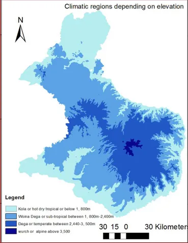
Gojam is located within the tropics where there is no significant variation in day length and the angle of the sun throughout the year. As a result, average annual temperature in the region are high and variations low. Although latitude mainly influence the overall temperature, the great variations in altitude and slope aspects also have very significant effects on regional microclimates and temperature. Traditional climate classification zone of the region based on elevation is Kola or hot dry tropical between 1500-1800m above sea level, Woina Dega or sub-tropical (1800-2400m above sea level), Dega or temperate (2440-3500m above sea level), and wurch or alpine (over 3500m above sea level) with mean annual temperatures of less than 10°C and rainfall less than 900mm. The most dominant crop in this climatic zone is Barley (Tegene 2002; FAO 1995; Mengistu 2006). Highlands above an altitude of 1500m experiences relatively cool temperature conditions in contrast to the lowlands (Figure 6).

(35)

23 Figure 6 Climatic regions of the study area depending on elevation

The climate of Gojam, Ethiopia is mainly controlled by the seasonal migration of the Inter-tropical Convergence Zone (ITCZ), which follows the position of the sun relative to Earth and the associated atmospheric circulation, in conjunction with the

country’s complex topography.

(36)

24 According to National Meteorological Agency there are three seasons in the region: Bega (dry season) from October to December, Belg (small rainy season) from February to May and Kiremt (main rainy season) from June to September (Babu 2009). The Belg rains begin when the Saharan and Siberian High Pressures are weakened and various atmospheric activities occur around the Horn of Africa. Low-pressure air related to the Mediterranean Sea moves and interacts with the tropical moisture and may bring precipitation to the region (Seleshi and Zanke, 2004). The high pressure in the Arabian Desert also pushes that low-pressure air from south Arabian Sea into mid- and southeast Ethiopia, which in turn, creates the Belg rains. The beginning of the Belg rain is also the period when the Inter-tropical convergences zone (ITCZ) begins to reach south and southwest Ethiopia in its south-north movement (Wolde-Georgis et al., 2000). For example, the creation of strong low pressure and cyclones in the southern Indian Ocean reduces the amount and distribution of rainfall in Ethiopia. The small rains also contribute to increased pasture for domestic and wild animals. Normal Belg rainfall adds moisture to the soil, enabling land preparation for the Kiremt or summer planting. The short rainy season, the Belg is the result of moist easterly and southeasterly winds and produces rains in March, April and May.

According to many previous studies and National Meteorological Agency of Ethiopia, ENSO has a great impact on Ethiopian, Gojam weather and climate variability (Bekele 1997; Wolde-Georgis et al., 2000). A negative sea surface temperature anomalies (SSTA) or La Niña is strong associated with rainfall deficiency in Belg and excess rainfall in Kiremt season; while, a positive SSTA or El-Nino is mostly associated with normal and above-normal rainfall amounts in Belg and deficiency of rainfall in Kiremt season. Furthermore, the National Meteorological Agency also realized that the sea surface temperatures (SSTs) in the Indian and Atlantic oceans also affect the region weather and climate variability. Most of the drought years are associated with El-Nino events; however, most of wet/flood years are associated with La-Nina episodes.

(37)

25

MATERIALS AND METHODS

4 Gridded datasets derived from climate data

4.1

Monthly mean maximum, minimum temperature and rainfall data were collected from National Meteorological Agency of Ethiopia. These data were also recorded from 15 Meteorological station placed in the study area for agricultural or rainy seasons (February -September)during the period 2000-2008 (Table 2; Figure 7). Three variables are analyzed in this study: mean monthly, seasonal and yearly rainfall, maximum and minimum temperature. The meteorological stations were irregularly distributed over the

study area and doesn’t represent the whole region well. There were a few data gaps and

removed by averaging data from the nearest neighbor stations.

Preparation of gridded climate maps was made by interpolation of these records based on the longitude, latitude and elevation of the weather stations. Use of elevation as secondary information for modeling gridded maps was not that much important but the relief or topography of study area has a bit influence on the spatial patterns of climate parameters. The magnitude of elevation ranges from 639 m to 4038 m. The general increase in precipitation with elevation is well known, it is due to fact that hills are barriers to moist airstreams, forcing the airstreams to rise and they act as high-level heat sources on sunny day.

Different interpolation methods were tried in order to increase the prediction accuracy such as inverse distance weighting (IDW), simple kriging, Universal kriging and ordinary kriging. Ordinary kriging method was the best for this study and all raster maps of seasonal precipitation for the study region were constructed using the geostatistical interpolation method known as ordinary kriging (OK). OK relies on the spatial correlation structure of the data to determine the weighting values instead of weighting nearby data points by some power of their inverted distance.Ordinary kriging is an effective spatial interpolation and mapping tool, because it honors data locations provides unbiased estimates at unsampled locations, and provides for minimum estimation variance, i.e. a best linear unbiased estimator (Jantakat and Ongsomwang, 2011).

(38)

26 Stations Longitude

(°E)

Latitude (°S)

Altitude (m)

Rainfall (mm) Temperature (oC)

Belg ( Feb-May)

Kiremt

(Jun-Sep)

Belg ( Feb-May)

Kiremt

(Jun-Sep)

Motta 37.52 11.05 2440 34.01 220.53 23.11 22.21

Debre Work 38.08 10.44 2740 38.72 187.21 9.42 22.99

Adet 37.28 11.16 2080 25.21 210.3 29.02 23.69

Ayehu 36.55 10.45 1725 54.94 211.91 31.36 24.33

Zege 37.19 11.41 1800 14.5 336.12 31.09 26.42

Bahar Dar 37.25 11.36 1770 22.19 321.53 29.63 25.35

Yetemen 38.08 10.2 2060 37.59 255.99 26.01 22.14

Gundil 37.04 10.57 2540 61.13 473.23 24.14 19.88

Dengay Ber 37.33 10.43 2800 58.55 415.72 24.44 18.92

Deke

Istifanos 37.16 11.54 1795 11.73 309.9 28.84 25.56

Wegedade 37.13 11.18 2000 39.2 213.68 29.29 26.00

Abay Sheleko 38.41 10.21 2000 54.86 238.96 29.74 27.29

Elias 37.28 10.18 2140 50.82 337.76 29.17 22.42

Shebelberenta 38.2 10.27 2000 40.31 198.16 27.51 23.45

Yetnora 38.09 10.12 2540 38.62 215.42 24.63 19.84

(39)

27 Figure 7 Distribution of the meteorological stations and Administrative regions in Gojam

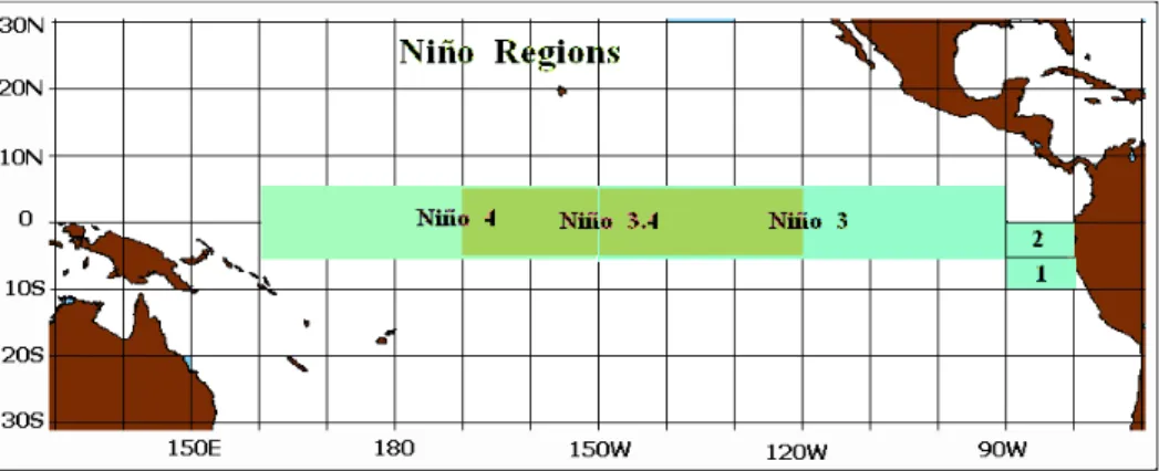
Figure 8 Geographical extent of the currently defined El Niño regions

Source:http://www.cgd.ucar.edu/cas/catalog/climind/TNI_N34/index.html; accessed 3 November, 2011

Gridded datasets derived from satellite data

4.2

(40)

28 requirement quality assessment also processed. NDVI pixels that fell below the acceptable QASDS quality level were deleted and flagged. The 16-days composite NDVI data sets were generated using a maximum value composite (MVC) procedure, which selects the maximum NDVI value within a 16-day period for every pixel. This procedure is used to reduce noise signal in NDVI data due to clouds or other atmospheric factors. The monthly NDVI raster map and others such as maximum, minimum and mean NDVI values were extracted by averaging the 16-composite. Negative NDVI values indicate non-vegetated areas such as snow, ice, and water. Positive NDVI values indicate green, vegetated surfaces, and higher values indicate increase in green vegetation.

Digital terrain model also used from United States Geological Survey (USGS) for pre-processing of satellite data and the supplementary statistical analysis in the main part of the study

Satellite system Sensor Spatial resolution

Temporal resolution

Time-period/ Acquisition date

NASA MODIS Terra MOD13Q1

250m NDVI 16 day composite From 2000-2008

Table 3 Satellite data used in the study

Although the Normalize difference vegetation index (NDVI) value classification is not specific, depending on previous some studies the vegetation condition of the region classified as High vegetation (values above 0.5), medium vegetation (from 0.292 - 0.5), low vegetation (0.166- 0.292), no vegetation ( from 0.1 -0.166) and water body (USAID, 2006; USGS 2011; USGS & USAID, 2005).

General statistical analysis of vegetation or biomass

4.3 condition

(41)

29 value of a pixel-level Cv over time relates to increased dispersion of values, not increase NDVI; similarly a negative Cv means decreasing dispersion of NDVI around the mean values, not decreasing NDVI.

Source: Bai et al. (2005) and Tucker et al. (2005)

Max-Min NDVI NDVI CV Interpretation of biomass variation

+ + Increase of biomass but unstable

- + Decrease of biomass but unstable

+ - Increase of biomass, stable

- - Decrease of biomass, stable

(42)

30

General methodological framework

4.4

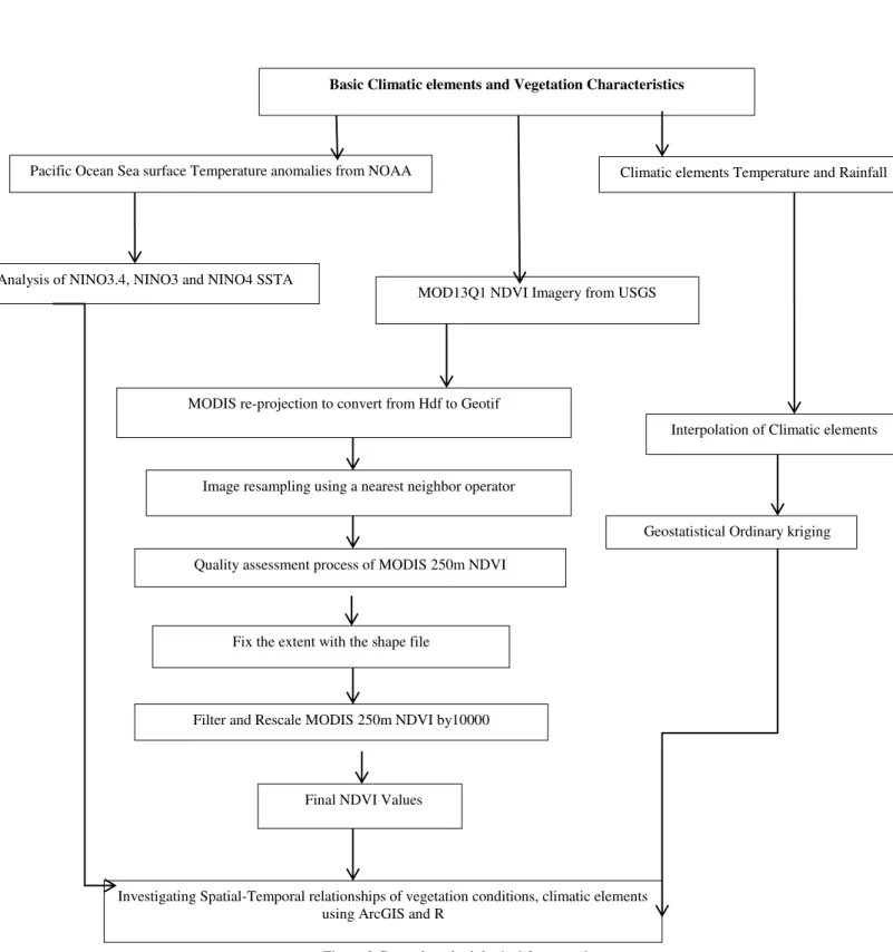
Figure 9 General methodological framework

Pacific Ocean Sea surface Temperature anomalies from NOAA Climatic elements Temperature and Rainfall

MOD13Q1 NDVI Imagery from USGS

Interpolation of Climatic elements MODIS re-projection to convert from Hdf to Geotif

Quality assessment process of MODIS 250m NDVI Image resampling using a nearest neighbor operator

Fix the extent with the shape file

Filter and Rescale MODIS 250m NDVI by10000

Final NDVI Values Analysis of NINO3.4, NINO3 and NINO4 SSTA

Geostatistical Ordinary kriging

Investigating Spatial-Temporal relationships of vegetation conditions, climatic elements using ArcGIS and R

(43)

31

RESULTS AND DISCUSSION

5 Spatial and temporal variation of Mean monthly NDVI for

5.1 Belg and Kiremt season

Generally, there is high vegetation coverage in Kiremt season (June, July, August and September) than Belg (February, March, April and May) from the period 2000 to 2008 due to good amount of rainfall in Kiremt season for plants or crop to grow. Relating to the altitude there is better vegetation coverage in the central part of the region, around choke mountain (the highest plateau of the region) in both seasons. In the other hand, there is less vegetation coverage in the eastern periphery of the region while, better vegetation coverage in the western part of region( Figure 10 and Figure 43). From seasonal quantitative analysis of vegetation coverage in both seasons as shown in (Table 5 and Table 6) there is 77.14 % highest high vegetation coverage class in the year 2002 Kiremt season. Yearly Kiremt season high vegetation coverage class from highest to lowest 2002 (77.14 %) and 2003 (66.59%) consecutively. Highest Kiremt season medium vegetation coverage class is in 2003 (23.24%) while, lowest medium vegetation coverage class and low vegetation coverage is in 2002 (12.74%).

In the Belg season the highest high vegetation coverage class year is 2007 (2.55%) and lowest high vegetation coverage class year is 2004(0.48%). The highest medium vegetation coverage class year is 2000 (58.15%) while, the lowest year 2003 (26.69%). The highest low vegetation class also in 2003 (61.91%).

(44)

32 and rainfall west, south, north west and south west part of region(Figure 13, Figure 15, Figure 16, Figure 17 and Figure 43).

(45)

33 Figure 11 Illustration maps of mean monthly NDVI in rainy season for 2008 La Nina year

(46)

34 Figure 12 Illustration maps of mean monthly NDVI in rainy season for 2002 El Niño year

(47)

35

(48)

36

(49)

37

Figure 15 Mean yearly vegetation coverage for rainy season from 2000 - 2008

Quantitative analyses of vegetation coverage in Belg and Kiremt

5.1.1

season

The quantitative analyses vegetation coverage shows almost similar quantity of high vegetation coverage that ranges from 70-77 percent in Kiremt season. The medium and low vegetation coverage of Kiremt season also shows similar quantity in the nine years. The Belg season quantitative analyses show high quantity of medium and low vegetation coverage not high vegetation coverage as Kiremt season.

(50)

38 Table 5 Kiremt season quantitative vegetation coverage

Table 6 Belg season quantitative vegetation coverage

Spatial and temporal variation of mean seasonal rainfall in

5.2 Belg and Kiremt

Ordinary kriging considered to be the best methods, as it provided smallest RMSE and ME value for nearly all cases. Since the distribution of sample data points is uneven

and sparse IDW interpolation techniques quality is very less and doesn’t cover the whole

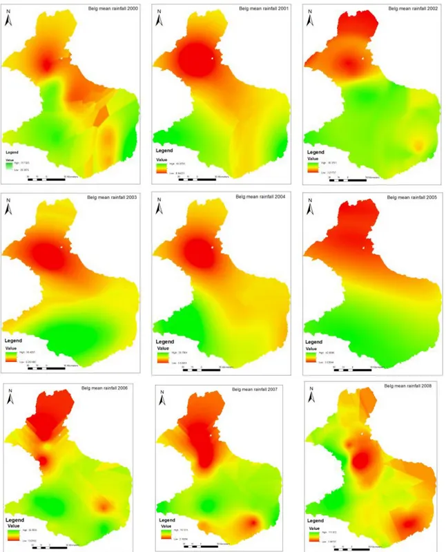
study area. Ordinary kriging was selected for this study based on how well it has performed on prior years data and because the statistical characteristics of the data in 2002 and 2003 make Ordinary Kriging the appropriate choice of estimator (Table 7). Exponential and stable type of models are used for ordinary Kriging interpolation of seasonal rainfall data ( Figure 49and Table 11).

% of vegetation coverage per year

Type of

vegetation 2000 2001 2002 2003 2004 2005 2006 2007 2008

High

Vegetation 72.66 68.83 77.14 66.59 75.90 70.10 72.02 74.59 76.61

Medium

Vegetation 17.03 20.85 12.74 23.24 13.97 19.69 17.78 15.19 13.19

Low

vegetation 0.302 0.32 0.17 0.24 0.18 0.26 0.23 0.27 0.23

No vegetation 0.09 0.10 0.10 0.11 0.10 0.10 0.10 0.10 0.10

Water 9.92 9.89 9.83 9.83 9.85 9.85 9.86 9.86 9.85

% of vegetation coverage per year

Type of

vegetation 2000 2001 2002 2003 2004 2005 2006 2007 2008

High

Vegetation 0.77 1.76 1.58 1.09 0.48 0.92 0.85 2.55 0.90

Medium

Vegetation 58.15 58.01 36.85 26.69 30.42 38.99 47.16 50.47 50.44

Low

vegetation 30.94 30.10 51.21 61.91 58.66 49.911 41.66 36.75 38.28

No vegetation 0.18 0.17 0.36 0.40 0.48 0.26 0.43 0.30 0.51

(51)

(52)

SPATIAL-TEMPORAL ANALYSES OF CLIMATE ELEMENTS, VEGETATION CHARACTERISTICS AND SEA SURFACE TEMPERATURE ANOMALY

Yitea Seneshaw Getahun

SPATIAL-TEMPORAL ANALYSES OF CLIMATE

SPATIAL-TEMPORAL ANALYSES OF CLIMATE ELEMENTS, VEGETATION

CHARACTERISTICS AND SEA SURFACE TEMPERATURE ANOMALY

ACKNOWLEDGEMENTS

ABSTRACT

SPATIAL-TEMPORAL ANALYSES OF CLIMATE ELEMENTS, VEGETATION

CHARACTERISTICS AND SEA SURFACE TEMPRATURE ANOMALY

KEYWORDS

ACRONYMS

TABLE OF CONTENTS

INDEX OF TABLES

INDEX OF FIGURES

INTRODUCTION

1

Motivation and Rational

1.1

Objectives

1.2

Assumptions

1.3

General Methodology

1.4

Organization of the thesis

1.5

LITERATURE REVIEW

2

Changes in land use and land cover pattern

2.1

Global Characteristics of Climate and Vegetation

2.2

2.2.1.1

Relationship between temperature, rainfall and vegetation

2.3

dynamics

Global climate variability and vegetation dynamics

2.4

General interactions between the ocean, atmosphere, earth

2.5

and climate variability

Analyses of vegetation dynamics and climate variability

2.6

using remote sensing

Geostatistics methods

2.7

Literature review summary

2.8

STUDY AREA

3

Description of the study area

3.1

MATERIALS AND METHODS

4

Gridded datasets derived from climate data

4.1

Gridded datasets derived from satellite data

4.2

General statistical analysis of vegetation or biomass

4.3

condition

General methodological framework

4.4

RESULTS AND DISCUSSION

5

Spatial and temporal variation of Mean monthly NDVI for

5.1

Belg and Kiremt season

Spatial and temporal variation of mean seasonal rainfall in

5.2

Belg and Kiremt