The Wagner hypothesis from the perspective of the Romanian economy

The Wagner hypothesis from the perspective

of the Romanian economy

Ana-Maria ŢEPUŞ Bucharest Academy of Economic Studies

anamaria.tepus@yahoo.com

Abstract. The study consists in determining a long term relationship between the size of the governmental expenses and the economic growth in Romania during the 2000-2010 period. By using the quarterly data of this period and the econometric techniques like the Granger causality, the co-integration analysis and VAR analysis, we have reached the conclusion that there is enough proof in favour of validating the Wagner law.

Keywords: Wagner law; Granger causality; the size of the governmental sector.

JEL Codes: E20, E21. REL Codes: 13C, 13K.

1. Introduction

The economic growth is one of the most fascinating subjects of the macro economy; the budgetary expenses represent one of the potential factors interesting to be studied in connection with the growth of an economy. The empiric studies regarding the impact of the budgetary expenses on the long term economic growth include the works of Romer(1) (1990), Barro(2) (1991), Levine and Renelt(3) (1992), Feder(4) (1997). Most of the studies utilize transversal data series for connecting the governmental expenses with the economic growth rates. The disadvantage of these studies is that the transversal analysis can identify the correlation but not the causality between the variables (Hsieh, Lai, 1994), because it provides only pooled estimations of the effect of the governmental sector size on the economic growth (Ghali, 1999), not allowing to identify the effect generated by each country.

The traditional OLS regression analysis is not enough for determining the sense of the causality(5). In any case, the value of the coefficient (which is a significant one) is compatible with the Keynes vision (causality from the budgetary expenses toward economic growth), the law of Wagner (causality from growth toward expense) and bidirectional causality between the two variables. The most indicated method for determining this relation is that of using the Granger(6) causality test.

The paper models the relationship between the GDP and the share of budgetary expenses in the GDP, by starting from the study of Ghali, correlated with the literature on the law of Wagner.

2. The level of knowledge regarding the Wagner hypothesis

The Law of Wagner(7) on expanding the activity of the state within the

economy, which states that the determining factor for increasing the size of the governmental sector is economic growth, continues to attract the econometricians. The critical examination of the most relevant articles (written during a time interval of four decades) that approaches this subject highlights the repeated divagations from the definition of Wagner on the activity of the state(8) and sacrificing the essence of formulating it with the view of presenting sophisticated econometric models, that will rival and even outrank those of the predecessors(9).

investment expenses; thus there was a question of the long term evolution of the governmental expenses and of the causes that generate their growth.

The Law of Wagner is brought back to our attention and it presupposes

the following:

1. Detects certain regularities on increasing the size of the governmental sector;

2. Including the public finances of the central and local administration as well as of the state enterprises within the definition of the governmental sector;

3. Wagner utilizes the term of “law” when referring to this regularities, stating also that its sense is imposed by the Wilhelm Lexis statistician (1911) (10).

4. Determining an absolute and relative growth of the public sector size, in comparison with the national economy, and a different growth rhythm from one branch to the other;

5. Including the traditional services (defence, justice, public order), as well as education, social assistance services and expenses generated by the modification of the economic structures(11);

6. Wagner was aware of the fact that by associating the growth of the governmental activity with the development of industrial companies raises the problem of the analysis period(12) and he is reserved in the attempt of finding this kind of limits. He also states that there are no specific limits regarding the contribution of the economic and cultural progress on the growth of the governmental sector.

The law of Wagner offers two possibilities of expanding the research in the field of measuring the growth of governmental expenses:

 It does not present an articulate model of the growth process of the of the governmental process within which the cause and effect have to be clearly defined;

 The agents involved in this dynamic process are not clearly identified. Rowley and Tollison (1994) state the hypothesis of Wagner is consistent with the comparative advantage doctrine. Wagner brings to the table the complementarity between the growth of the industrial sector and the growth of the demand for public services with economic character (like transportation and other communication networks, waste management and the other services provided in general by the state agencies). Therefore, Stigler (1986) expands the idea and explains the long term demand for the governmental expenses.

private industry. Instead the governmental sector is seen as a planner of the economy working for the public interest and it takes intelligent decisions that would promote the industrial development in line with taking over and developing the basic public utilities.

The rather vague hypotheses of the Wagner theory do not satisfy the rigors of the partisans of the present economic models that use statistic techniques very advanced for testing, yet the advantages do not counter weight the survival power of the theory.

The numerous testing of the theory have focused on the following aspects:

a) measuring the size of the governmental sector

 there are approximately 14 different techniques for measuring the governmental expenses, starting with the restrictive definitions (which excludes the transfers or expenses related to defence) up to the very detailed definitions (that include all the expenses that can be found in the public accounts(13));

 misinterpretation of the Wagner theory (which also includes the public utilities in the governmental sector); omission of the influence of public enterprises can be seen as being intentional;

 three possibilities of referring to increasing the variable which depends on the governmental sector (G) were identified;

‐ the stricto sensu increase of the governmental sector (G);

‐ increase of the governmental sector share within the GDP (G/Y); ‐ increase of the public expense value per capita (G/N).

Each of these possibilities is consistent with a certain interpretation of the Wagner law. By corroborating these options with the 14 modalities of measuring the governmental expenses we reach a result of 42 possible dependent variables.

b) independent variables

 gross national income/GDP;

 changes regarding the population;

 the degree of industrialization;

 the degree of urbanization.

Difficulties: Wagner draws the attention in regard to the analysis period of his law; therefore in a period characterized by deindustrialization it is called into question if the governmental activity, as an important component of the services sector, would be influenced by the productivity lag associated with the

Baumol effect(14), a fact which introduces a structural element in the analysis,

c) data series

 focus on comparisons between the developed countries and the emerging markets, as well as between the developed countries (there is a uniformity regarding the growth levels of the G/Y ratio in the Western-European economies, yet there is a difference between G/Y of Sweden vs. Japan).

d) testing methods

 multiple regression (it presents the deficiencies which are trying to be resolved by utilizing more complex models);

 co-integration – the one most consistent with the hypothesis of Wagner (who states that there isn’t necessarily a cause-effect type of relationship between the economic development and the increase of the governmental expenses(15)), that is trying to identify the existence of a long term relationship between the variables, which cannot be pointed out through the multiple regression method(16);

 later on the presence/direction of a causality is determined => the Granger causality test(17).

The various tests applied to the Wagner law are criticized: on the one hand, the omission (the superficial approach of the governmental activity significance), and on the other hand, commission (utilizing excessively the econometric techniques, which led to fake precision in formulating the causal relationship identified between the governmental activity variable and other macroeconomic variables).

3. Data and methodology

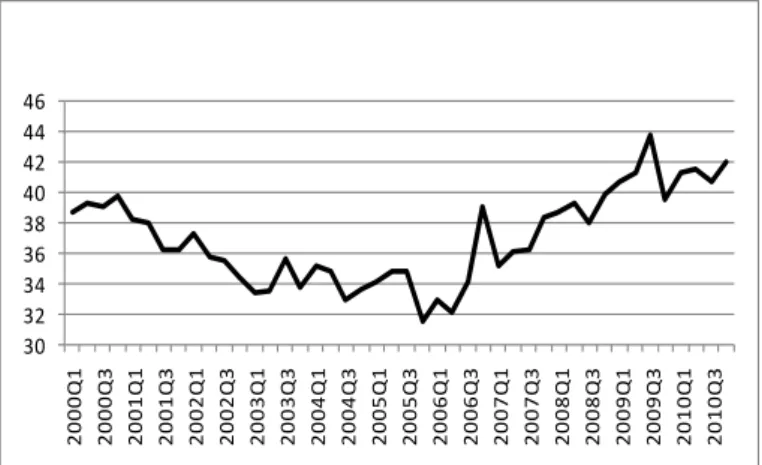
In order to present for Romania the accuracy of the law of Wagner, we have utilized the data that have a quarterly frequency available on the EUROSTAT web site, for the following variables in the 2000-2010 period:

 y = the real ration of governmental expenses in the GDP;

 x = real GDP (expressed in the prices of 2005);

Due to the fact that the quarterly data present an accentuated seasonality, the variables where de-seasoned by using the TRAMO/SEATS procedure, available in Eviews5.

We decided to utilize the quarterly data instead of the annual ones, for two reasons:

 from the perspective of efficiency and significance of the statistic tests, the annual data series is too restricted to allow obtaining trustworthy results;

 the variables that characterize the Romanian economy in the 1990-2010 period have serious structural gaps and significant trend reversals, which makes an analysis for this time horizon by utilizing the annual data to be not feasible.

30 32 34 36 38 40 42 44 46

2

000Q

1

2

000Q

3

2

001Q

1

2

001Q

3

2

002Q

1

2

002Q

3

2

003Q

1

2

003Q

3

2

004Q

1

2

004Q

3

2

005Q

1

2

005Q

3

2

006Q

1

2

006Q

3

2

007Q

1

2

007Q

3

2

008Q

1

2

008Q

3

2

009Q

1

2

009Q

3

2

010Q

1

2

010Q

3

15000 17000 19000 21000 23000 25000 27000 29000 31000 33000 35000 2000 Q 1 2000 Q 3 2001 Q 1 2001 Q 3 2002 Q 1 2002 Q 3 2003 Q 1 2003 Q 3 2004 Q 1 2004 Q 3 2005 Q 1 2005 Q 3 2006 Q 1 2006 Q 3 2007 Q 1 2007 Q 3 2008 Q 1 2008 Q 3 2009 Q 1 2009 Q 3 2010 Q 1 2010 Q 3

Figure 2. RealGDP (million lei, for the average prices of 2005) – series adjusted in a seasonal manner

3.1. The regression method utilized to determine the correlation between the GDP and the governmental expenses

The easiest method for determining the potential correlations between the analysed variables is the classic linear regression; unfortunately, its hypotheses are very restricted and such a model can only signal the presence of a linear correlation. Furthermore it is improper to speak about the regression as a method for determining the existence of causality.

Nevertheless, the estimation of a regression model can provide clues regarding the existence of a possible long term relationship between the variables.

In the following, we have tested the law of Wagner in the formal sense of Mann (1980), in accordance to which the share of governmental expenses within the GDP can be expressed according to the real GDP:

t t

t x

y 







ln _{0 1} , where



In order to validate the law of Wagner, the₁ coefficient needs to be significant and furthermore₁ 0.

3.2. Stationary and co-integration tests

Practically, the two time series are co-integrated if they have the same order of integration, yet their linear combination has a lower integration order.

For example, we can have two integrated series of order one, e.g. the order one differences are stationary, yet there can be a linear combination of the two series which should be stationary, namely an order 0 integral.

The stationary test was carried out through the Augmented Dickey-Fuller

general procedure, by estimating the following regression model:



t t y y u

y

1 1 1

0  ( 1) 

 , where y_t is the variable for

which the stationary is verified, and p is the optimum number of lags utilized to verify the possible auto-correlations of higher order. The optimum number of lags utilized for the ADF test can be chosen based on maximizing the Schwarz informational criteria (SIC).

The hypotheses of the test are the following      1 : 1 : 0   A H H

, rejecting the null

hypothesis equivalent with accepting the stationary r.

We have Y_t (lny_t lnx_t)' the vector of the time series so that lny_tI(1)

and lnx_tI(1). Then lny_t and lnx_t are co-integrated if there is a  matrix so

that '_{Y I}(0) t

 .

In order to be able to check if the two data series are co-integrated we have applied the Johansen (1991) procedure.

Therefore, we have a VAR model of the order p:

t p t p t

t AY A Y

Y  _{1 1}... _  , where Y_t (lny_t lnx_t)' is the vector of the

two studied variables, integrated of order one, and



The above VAR model can be rewritten:

t i t p i i t

t Y Y

Y    

    



1 , where



    p i i I A 1

and



     p i j i i A 1 .

The Granger representation theorem states that if the matrix of the  coefficients has the rank rk, then we have matrix,M(kr), each

having rank k, so that 



The Johansen method consists in estimating the  matrix from a VAR model without restrictions and afterwards testing the restrictions that results from taking a rank rk.

In fact, the following possible situations are being tested:

 vector Y_t does not have a deterministic trend, and the co-integration equations do not have an absolute term: _1 ' _t1

t Y

Y

 ;

 vector Y_t does not have a deterministic trend, and the co-integration equations have the absolute term: ( ' _{1 0})

1   

Yt_ Yt_ ;

 vector Y_t has a deterministic trend, and the co-integration equations only have absolute term: Y_t1 ('Y_t1₀)_t₀;

 vector Y_t and the co-integration equations have a linear trend:

0 1

0 1 '

1 ( t   ) t

t Y t

Y    

 _{ } ;

 vector Y_t has a square trend, and the co-integration equations have a linear trend: Y_t1 ('Y_t1₀₁t)_t(₀₁t).

3.3. The Granger causality

We can determine the existence of a long term relationship between the GDP and the governmental expenses by testing the bi-varied Granger causality.

The Granger causality between two variables refers to the manner in which the past values of a variable can be utilized in order to explain the values of the other variables.

In our situation, testing the Granger causality is reduced to estimating the regression models:

t l t l t

l t l t

t y y x x

y 













ln _{0 1 1 1 1}

t l t l t

l t l t

t x x y y u

x   ln _ ... ln _  ln _ ... ln _ 

ln











The null hypothesis for which the validity is being tested is

0 ...

: ₁

0   l 

H





have tested the fact that ln does not cause Granger y lnx.

Before applying the test we need to determine the correct VAR model(19). Between a VAR model with dummy variables and one with “forged” periods, the second one seems to be a model with better specifications. During the causality testing, the results are sensitive to the number of lags utilized in the analysis.

3.4. The VAR model for the relationship between the governmental expenses and the GDP

In order to express the magnitude and the sense of the GDP-governmental expenses causality relation, we have estimated the VAR(p) model:

t p t p t

t AY A Y

Y  _{1 1}... _  , where Y_t (lny_t lnx_t)' is the vector of the

two studied variables, integrated of order one, and



The results of such a model show the orientation of the link between the two variables as well as the significant temporal delay which describes this link.

4. Results

Due to the fact that we have worked with quarterly data, it is normal that there would be a temporal delay between the GDP evolution and the evolution of the governmental expenses; because of this we have estimated the following types of regression models:

t k t

t x

y 







ln _{0 1} , where k is the temporal delay and



Table 1

Results of the regression models with lags

k 1 SE (1) Statistic t Prob t R2 Statistic F Prob F

0 0.128 0.077 1.658 0.105 0.061 2.749 0.105

1 0.166 0.077 2.165 0.036 0.103 4.685 0.036

2 0.214 0.075 2.863 0.007 0.170 8.196 0.007

As it can be observed from the results of the estimated models, there is a significant direct correlation between the GDP and the share of governmental expenses in the GDP, but this relation does not have a mechanism of immediate communication, which suggests the existence of a potential long term correlation.

In other words, it is expected that the law of Wagner should have empiric verification for Romania, as there is a positive relation between the two variables.

Nevertheless the classic regression model does not provide robust results, if the two series are not stationary, otherwise having the possibility of obtaining a false regression.

In order to test the stationary of the two series, as well as their integration order, we have used the ADF test, above described, for the level series and for the order one differences.

Table 2

Unit root test for lny, lnx, lny, lnx

lny lny lnx lnx

 - 1 -0.143 -1.349 -0.023 -0.427

Statistic t -1.620 -3.597 -1.770 -3.296

Critical value (5%) -2.931 -2.933 -2.933 -2.933

2

adj

R _{0.037 0.673 0.346 0.194}

Statistic F 2.625 82.256 11.836 10.865

Prob F 0.113 0.000 0.000 0.002

Due to the fact that the probability associated with the null hypothesis of unitary root is lower than the usual level of significance of 5%, we reject the non-stationary hypothesis, therefore the order one differences of the two series are stationary and as a consequence the lny_t and lnx_t series have the same

integration order (lny_tI(1) and lnx_tI(1)).

Table 3

Results of the co-integration tests

Data trend: None None Linear Linear Quadratic Test type No intercept Intercept Intercept Intercept Intercept

No trend No trend No trend Trend Trend

Trace 1 2 2 1 0

Max-Eig 0 2 2 0 0

Table 4

Results of the Granger causality test for l _{= 5}

The causality F-Statistic P-value

GDPGovernmental expenses 4.30021 0.005

Governmental expenses GDP 1.96548 0.11502

Because the probability of the Granger test is lower than the level of significance only for the first causality relationship, the conclusion is that the Granger causality relationship is unique, and the orientation is given from the GDP toward the governmental expenses and not the other way around.

Taking into account that we have established that there is a significant Granger causality relationship in the GDPGovernmental expenses orientation, we can estimate a VAR(p) model in order to evaluate the direction of this causality relationship. We have estimated for this a VAR model without restrictions and a VECM (Vector Error Correction Model), to take into consideration the co-integration relationship which exists between the two series of data.

Taking into account the results of the Granger causality test, we chose the order for the two models p=4.

The VAR model

The VAR(4) Model has the following form:

                                             t t t t t t t t t t t t t t t t t t t t x x x x y y y y x x x x x y y y y y 2 4 44 3 23 2 22 1 21 4 24 3 23 2 22 1 21 20 1 4 14 3 13 2 12 1 11 4 14 3 13 2 12 1 11 10 ln ln ln ln ln ln ln ln ln ln ln ln ln ln ln ln ln ln                    

The results of the estimates are presented in the following table.

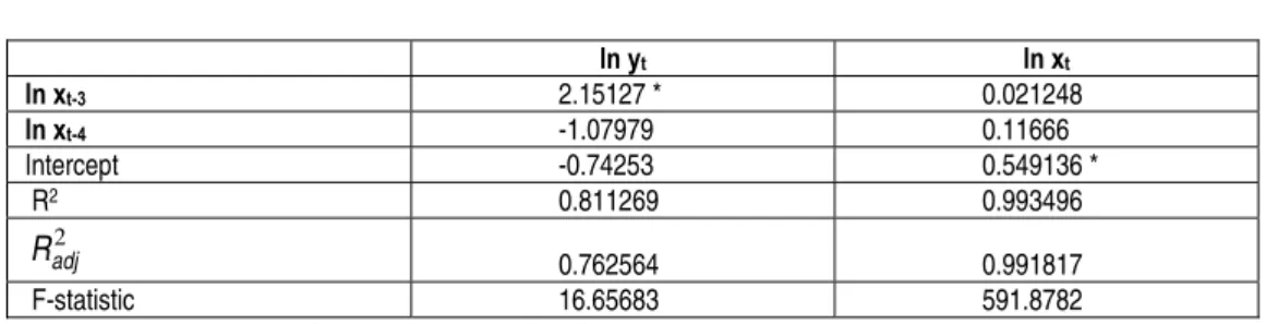
Table 5

Estimates of the VAR(4) model

ln yt ln xt

ln yt-1 0.396545 * -0.02393

ln yt-2 0.267232 0.022208

ln yt-3 0.12822 -0.05277

ln yt-4 0.043196 -0.02461

ln xt-1 -0.1818 1.429455 *

ln yt ln xt

ln xt-3 2.15127 * 0.021248

ln xt-4 -1.07979 0.11666

Intercept -0.74253 0.549136 *

R2 _{0.811269 0.993496}

2

adj

R _{0.762564 0.991817}

F-statistic 16.65683 591.8782

* - statistically significant with a probability of 95%

From the analysis of the coefficients of the estimated VAR(4) model we can observe a significant influence of the GDP on the governmental expenses, with a delay of three quarters, all the other coefficients are not significantly different from zero. The fact that this coefficient is positive symbolizes the existence of a direct relationship between the two variables, which is a validity clue of the Wagner law.

Also, the coefficients corresponding to the governmental expenses are not significant to any lag in the GDP equation, which is in accordance with the results of the Granger causality test.

Figure 3. The governmental expenses function of responding to a shock of the GDP

As it can be observed in the impulse-response graph, the governmental expenses react significantly to a shock of the GDP with a delay of at least three quarters.

The VECM model

The VECM(4) model has the following form:

The a,b,c coefficients are estimated based on a co-integration

relationship between lny_t and lnx_t.

In the above model the c coefficient describes, for the long term, the elasticity of the governmental expenses in relation to the Gross Domestic Product.

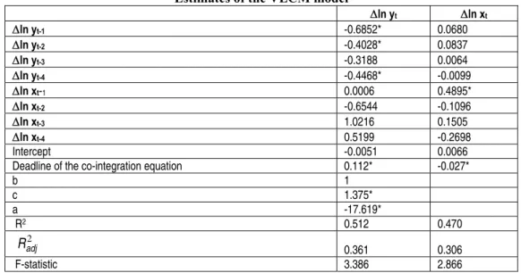
The results of the estimates are presented in the following table:

Table 6

Estimates of the VECM model

ln yt ln xt

ln yt-1 -0.6852* 0.0680

ln yt-2 -0.4028* 0.0837

ln yt-3 -0.3188 0.0064

ln yt-4 -0.4468* -0.0099

ln xt-1 0.0006 0.4895*

ln xt-2 -0.6544 -0.1096

ln xt-3 1.0216 0.1505

ln xt-4 0.5199 -0.2698

Intercept -0.0051 0.0066

Deadline of the co-integration equation 0.112* -0.027* b 1

c 1.375* a -17.619*

R2 _{0.512 0.470}

2

adj

R _{0.361 0.306}

F-statistic 3.386 2.866

* - statistically significant with a probability of 95%

The results of this model’s estimates show a direct and significant relationship between the governmental expenses and the GDP.

This long term influence can be observed in an even clearer manner from the impulse-response graph, as the governmental expenses react in a significant manner to a shock of the GDP, even for a longer period.

An interesting conclusion can be drawn from the value and sign of the long term elasticity coefficient (c=1.375), which suggests a direct relationship between the dynamic of the Gross Domestic Product and the dynamic of the share of the governmental expenses within the GDP.

5. Conclusions

The law of Wagner, which postulates the existence of a causality relationship between the GDP and the evolution of the governmental sector, is one of the subjects that are intensely studied by the economists. The difficulty of the empiric verification consists in the fact that there are various functional forms of this causality relation, and the econometric methods that were used over time provided contradictory results.

In this study we have verified the validity of this law for the Romanian economy, using the quarterly data belonging to the 2000-2010 period. The results obtained from applying certain varied econometric techniques are consistent with those obtained by other researchers in this area.

The data series of the governmental expenses and of the GDP series are integrated of order one, and there is a significant co-integration relationship between them. Furthermore, we can establish the existence of a Granger causality relationship between the size of the governmental sector and the GDP, but this causality is unidirectional, manifesting from the GDP toward the governmental sector. The fact that as a following of the applied tests there was no significant causality from the dimension of the governmental sector toward the GDP is an illustration of the fact that the effects of the governmental policies did not manifest in the direction of generating economic growth, the latter actually having exogenous causes, because of the favourable international and local context(20).

Notes

(1)

Paul Romer, Stanford University- California.

(2)

Robert Barro, Harvard University- Cambridge, MA; one of the most influential economists at global level in accordance with IDEAS- Research Papers in Economics.

(3)

Ross Levine (World Bank) and David Renelt (Harvard University, Cambridge, MA).

(4)

Kris Feder, Leon Levy Institute- New York.

(5)

When the economic growth is regressed based on the governmental expenses, the researches tend to interpret the result as being a confirmation of the causality from the last toward the first variable.

(6)

Clive Granger (1934-2009), winner of the Nobel prize for economy in 2003; the results of this technique shows that the size of the governmental sector determine in a positive manner the economic growth – which supports the Keyenes vision (Ghali, 1999, in the study that focuses on the OCDE countries); Hsieh and Lai (1994), on the other hand drew the conclusion that there is no proof of the presence of a certain Granger causality from the governmental expense toward the GDP growth PIB per capita for the G7 countries.

(7)

Named after the German economist Adolph Wagner (1835-1917).

(8)

“The appearance of an industrialized modern society entails a political pressure having the purpose of supporting the social progress and the allocation by the industry of certain higher amounts for promoting the social aspects” (Wagner) – “law” formulated for the first time in 1883, finalized in 1911 and utilized for the first time in English in 1958 by the American economist of German origins Richard A. Musgrave (economist-researcher of FED and a professor at Harvard University).

(9)

Wahab (2004 – “Economic Growth and Expenditure: evidence from a new test specification”) tried to point out the effects of a increasing or decreasing rhythm of the economic growth for the OCDE, EU and G7 countries for the 1950-2000 period; it established that the Wagner law is complied with only for the EU countries (in regard to the other countries, it determined that the size of the governmental sector increases with a rhythm lower than the one of the economic growth and it decreases more than proportional along with the decrease of the economic growth rhythm). Contrary the study of Kolluri et al. (2000) focuses on the relationship between the economic growth and certain components of the public expenses (the dependent utilized variables are: total budgetary expenses, total governmental consumption and the expenses with the governmental transfer) of the G7 countries and it certifies that the law of Wagner is respected. For the UK especially, the law of Wagner was confirmed for all the categories of public expenses taking into account the positive sign of the coefficients.

(10)

It utilizes the term of “law” with the meaning of “uniformity observed from the empiric perspective”, and not with the meaning applied by Pareto to the law of income distribution.

(11)

The increase of the governmental sector is also associated with the extensive use of the legislation regulating the economy.

(12)

Along which this empiric uniformity is being verified.

(13)

(14)

A phenomena described in the 60’s, which implies salary increases in the areas that have not experienced an improvement of the labor productivity, as an answer to the salary increases in areas that have registered an increase of the labor productivity.

(15)

The presence of co-integration does not imply causality.

(16)

The interpretation is the following one: once we establish the integration degree of the independent variables , we can establish the degree of co-integration of the series (if a linear combination of the integrated series is very static).

(17)

The verification of the law depends on verifying the causality direction of the co-integrated data series, namely it has be from the economic development variable toward the governmental activity variable.

(18)

Technological Institute of Western Macedonia, Department of Financial Informatics.

(19)

A VAR model specified in the correct manner needs to take into consideration the data gaps.

(20)

Namely, taking into account the very globalized international economic context and the weak industrialization of the Romanian economy vs. the one of the developed European states, the increase of the budgetary expenses was actually translated into an increase of the budgetary deficit; the low share of the capital expenses led to increasing the external deficit (the relationship is 1 p.p. budget deficit growth binds a 0.75 p.p. external deficit growth), attracting thus a reaction contrary to that originally expected - namely boosting the imports and depreciating the national currency; there were measures taken to fight against inflation (increasing the monetary interest rate) which generated a deceleration of the Romanian economy.

References

Andrei, T., Lefter, V., Oancea, B., Stancu, S. (2010). “A Comparative Study of Some Features of Higher Education in Romania, Bulgaria and Hungary”, Romanian Journal for Economic Forecasting, Institute for Economic Forecasting, Vol. 2, July, pp. 280-294 Barro, R.J. (1990). “Government spending in a simple model of endogenous growth”, Journal

of Political Economy, 98, pp. 103-S124

Barro, R.J. (1991). “Economic growth in a cross section of countries”, Quarterly Journal of Economics, 106, pp. 407-44

Cosimo, M. (2010). “Wagner’s law and augmented Wagner’s law in EU-27. A time-series analysis on starionarity, cointegration and causality’, C.R.E.I. Working Papers, No. 5 (October 2010)

Dritsaki, C., Dritsaki, M. (2010). “Government Expenditure and National Income: Causality Tests for Twelve New Members of E.E.”, Romanian Economic Journal, Year XIII, No. 38, December 2010

Feder, G. (1983). “On exports and economic growth”, Journal of Development Economics, 12, pp. 59-73

Hsieh, E., Lai, K. (1994). “Government Spending and Economic Growth: The G- 7 Experience”, Applied Economics, Vol. 26, pp. 535-542

Levine, R., Renelt, D. (1992). ”A sensitivity analysis of cross-country growth regressions”, American Economic Review, 82, pp. 943-63

Romer, P.M. (1990). “Endogenous technological change”, Journal of Political Economy, 98, pp. 71-102

Wagner, A. (1890). Fiannzwissenschaft (3rd ed.), partly reprinted in (Eds.) R.A. Musgrave and A. T. Peacock, Classic in the Theory of Public Finance, Macmillan, London, 1958

Wahab, M. (2004). “Economic growth and expenditure: evidence from a new test specification”, Applied Economics, 36, pp. 2125-2135