http://dx.doi.org/10.7494/OpMath.2017.37.3.403
SUFFICIENT CONDITIONS FOR OPTIMALITY
FOR A MATHEMATICAL MODEL
OF DRUG TREATMENT
WITH PHARMACODYNAMICS
Maciej Leszczyński, Elżbieta Ratajczyk, Urszula Ledzewicz,
and Heinz Schättler
Communicated by Marek Galewski
Abstract. We consider an optimal control problem for a general mathematical model of drug treatment with a single agent. The control represents the concentration of the agent and its effect (pharmacodynamics) is modelled by a Hill function (i.e., Michaelis-Menten type kinetics). The aim is to minimize a cost functional consisting of a weighted average related to the state of the system (both at the end and during a fixed therapy horizon) and to the total amount of drugs given. The latter is an indirect measure for the side effects of treatment. It is shown that optimal controls are continuous functions of time that change between full or no dose segments with connecting pieces that take values in the interior of the control set. Sufficient conditions for the strong local optimality of an extremal controlled trajectory in terms of the existence of a solution to a piecewise defined Riccati differential equation are given.
Keywords:optimal control, sufficient conditions for optimality, method of characteristics, pharmacodynamic model.
Mathematics Subject Classification:49K15, 93C15, 92C45.
1. INTRODUCTION
We consider optimal control problems for drug treatment. The controls u in the formulation represent the dosages of various therapeutic agents while pharmacokinetic models (PK) describe the relations between the dosages of the agents and their concentrationsc in the blood stream (“what the body does to the drug”) and pharma-codynamic models (PD) describe the effects that the drugs have on the disease (“what the drug does to the body”). Generally, PK is modelled by low-dimensional linear differential equations with real eigenvalues [7]. Pharmacodynamic models, on the other
c
hand, are simply given by functional relations of the formϕ(c) that model the effect the concentration c has. Here both linear models (based on the log-kill hypothesis [17]) as well as Michaelis-Menten or sigmoidal functional relations are commonly used [10,13]. While there exists a large literature on optimal control of mathematical models for chemotherapy going back to the early papers by Swierniak [19] and Swan [18], even including papers with state-space constraints (e.g., [5]), in most of these papers pharmacodynamic relations are not included. Yet, these type of functional relations are highly nonlinear and thus the dependence of optimal controls on the specific relations used in the modeling becomes a mathematically nontrivial problem [8, 9, 15] which at the same time is of great practical interest. These changes thatpharmacometrics(i.e., both PK and PD) induce on the structure of optimal solutions are the scope of our research.
In this paper, we present results about the structure of optimal controls for a single chemotherapeutic agent when pharmacodynamics is modelled by a Michaelis-Menten type equation. This relation is based on enzyme kinetics and takes the form
Emax
c C50+c
, (1.1)
whereEmaxdenotes the maximum effect the drug can have andC50is the concentration for which half of this maximum effect is realized. These are standard parameters used in pharmacology to describe the effectiveness of drugs. This model, also called the
Emax-model in pharmacology, is appropriate for fast acting drugs that do not have a prolonged initial phase when the concentration builds up slowly. During such a phase the drug is still rather ineffective and a sigmoidal model would be more appropriate. Contrary to linear models of the formγc, a Michaelis-Menten form captures the typical saturation effects when the concentration becomes too large. As such it is the most commonly used model for PD in the industry. For simplicity, here we also do not include a pharmacokinetic model and thus identify the drug’s dosage with its concentration in the blood stream. Once more, this is a reasonable modeling assumption for fast acting drugs.
For a fixed therapy horizon, we consider the optimal control problem to minimize a weighted average of quantities related to the state of the disease or infection and the total amount of drugs administered. The latter is given by the integralRT
2. FORMULATION OF THE OPTIMAL CONTROL PROBLEM
We consider a general system of differential equations of the form
˙
x=f(x) + u
1 +ug(x), (2.1)
where f : D → Rn and g : D → Rn are continuously differentiable vector fields
defined on some domainD⊂Rn. The dynamics represents an abstract formulation
for chemotherapy with a single agent. The vector fieldf, called thedrift, describes the evolution of the system when no drugs are given (u≡0), while the vector fieldg, thecontrol vector field, in combination with the control term describes the effects of drug treatment. The variableu, thecontrolin the system, represents theconcentration
of the chemotherapeutic agent given. In this formulation we do not yet include a pharmacokinetic equation and thus identify the dosage with the concentration. The functional form used for the controlurepresents a Michaelis-Menten orEmax-model withC50 normalized to 1 and the constantEmax subsumed ing.
Controls are Lebesgue measurable functions u : [0, T] → [0, umax] defined over an a priori fixed therapy horizon [0, T] that take values in a compact interval [0, umax]. It follows from standard results on solutions of differential equations that for any
x0∈Dthe initial value problem for the dynamics (2.1) with initial conditionx(0) =x0 has a unique local solutionx(·;x0) which we call the corresponding trajectory. However, for general vector fieldsf andg there is no guarantee that this solutions will exist on all of [0, T].Admissible controls thus are only those controls for which this solution exists over the full therapy horizon. For an admissible control we then define the
objective functional J in the form
J =J(u) =αx(T) +
T
Z
0
βx(s) +γu(s)ds, (2.2)
whereαandβ aren-dimensional row vectors,α, β∈(Rn)∗, andγ is a positive real number. The term αx(T) represents a weighted average of the variables x at the terminal timeT (such as the total number of cancer cells at the end of therapy) while the integral term on the statexis included to prevent that this quantity would increase to unacceptably high levels in between. The integral of the control is the AUC-term of pharmacology and it is a measure for the side effects of treatment. Minimizing this quantityJ generates a compromise between two competing aims of treatment. On one hand, the aim is to reduce the statexwhich represents the severity of the disease or infection (e.g., tumor volume) and this requires to give as much drugs as possible. On the other hand, side effects need to be limited and so the aim also is to give as little drugs as possible. Clearly, the balance will be determined by the weightsα, β
andγin the objective and generally these coefficients are variables of choice which often need to be selected carefully to obtain a meaningful behavior.
We thus consider the following optimal control problem:
3. NECESSARY CONDITIONS FOR OPTIMALITY
The fundamental necessary conditions for optimality for problem [MM] are given by the Pontryagin maximum principle [12] (for some more recent references on optimal control, see [1,2,14]). Since the optimal control problem [MM] does not involve terminal constraints on the state, extremals are normal and without loss of generality we already define the Hamiltonian functionH for the control problem as
H : (Rn)∗×Rn×R→R,
(λ, x, u)→H(λ, x, u) =βx+γu+
λ, f(x) + u 1 +ug(x)
(3.1)
withhλ, vi=λvdenoting the inner product of a row vectorλwith a column vectorv. It follows from the Pontryagin maximum principle [12] that, if u∗ is an optimal
control and x∗ denotes the corresponding trajectory, then there exists a covector
λ: [0, T]→(Rn)∗ which is a solution to theadjoint equation,
˙
λ=−β−λ
Df(x) + u
1 +uDg(x)
(3.2)
with terminal conditionλ(T) =αsuch that the Hamiltonian H is minimized almost everywhere on [0, T] byu∗ along (λ(t), x∗(t)), i.e.,
H(λ(t), x∗(t), u∗(t)) = min
0≤v≤umax
H(λ(t), x∗(t), v). (3.3)
Controlled trajectories (x, u) for which there exists a multiplierλsuch that these conditions are satisfied are called extremals and the triples (x, u, λ) including the multipliers are called extremal lifts (to the cotangent bundle).
An important property for solutions to the optimal control problem [MM] is that optimal controls are continuous. More specifically, we have the following representation of optimal controls.
Theorem 3.1. Letu∗ be an optimal control with corresponding trajectory x∗ and let
λbe an adjoint vector such that the conditions of the maximum principle are satisfied. Then we have that
u∗(t) =
umax ifhλ(t), g(x∗(t))i ≤ −γ(umax+ 1)2,
q
−hλ(t),g(x∗(t))i
γ −1 if −γ(umax+ 1)
2≤ hλ(t), g(x
∗(t))i ≤ −γ,
0 if −γ≤ hλ(t), g(x∗(t))i.
(3.4)
Proof. We need to minimize the HamiltonianH as a function of the controluover the control set [0, umax]. Since
∂H ∂u =γ+
hλ, g(x)i
it follows thatH(λ(t), x∗(t), u) is strictly increasing inuif the function
Φ(t) =hλ(t), g(x∗(t))i (3.5)
is non-negative. In this case the minimum over the control set [0, umax] therefore is attained foru∗= 0. If Φ(t) is negative, then it follows from
∂2H
∂u2 =−
2hλ, g(x)i
(1 +u)3
that the HamiltonianH(λ(t), x∗(t), u) is a strictly convex function ofuonR. Hence
it has a unique stationary point and this point is the global minimum of the function. Solving ∂H
∂u = 0, the stationary point is given by
ust(t) =
s
−Φ(t)
γ −1. (3.6)
Depending on the location of ust(t) we have the following three cases: if ust(t)<0, then the function H(λ(t), x∗(t),·) is strictly increasing on [0, umax] with minimum
atu∗= 0; if 0≤ust(t)≤umax, then the global minimum lies in the control set and
thus u∗ is given by the stationary point, and ifust(t)> umax, then H(λ(t), x∗(t),·)
is strictly decreasing over [0, umax] with minimum at u∗ = umax. This proves the
result.
Corollary 3.2. Optimal controls are continuous.
Proof. Using the notation from the proof above, as long as Φ(t) is negative, the point
ust(t) where the HamiltonianH(λ(t), x∗(t),·) attains its minimum varies continuously
witht. For this case we can represent the control in the form
u∗(t) = max{0,min{ust(t), umax}} (3.7)
and thusu∗ is continuous as long as Φ(t) is negative. For Φ(t)≥0 the optimal control
is given byu∗ ≡0 which is also the optimal control for Φ(t)≥ −γ. Hence, optimal
controls remain continuous as Φ becomes nonnegative.
Thus optimal controls continuously change between the limiting valuesumaxand 0 and values that lie in the interior of the control set as the function Φ crosses the levels
−γ and−γ(1 +umax)2. We therefore call the function Φ the indicator function for the optimal control. Clearly, it is this function that determines the optimal controls. For example, we have the following result:
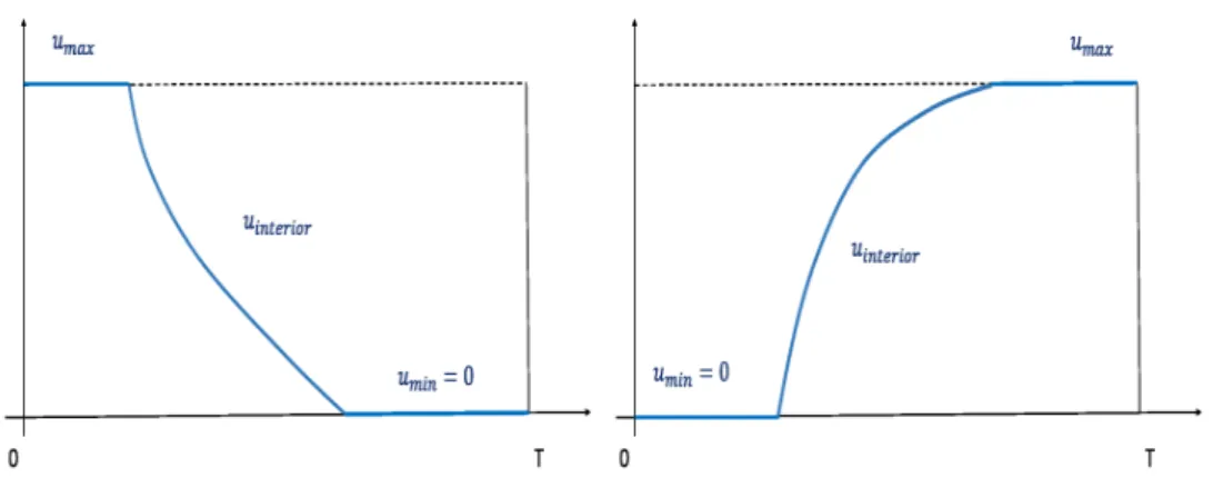
Proposition 3.3. If the indicator function Φ is strictly increasing on [0, T], then optimal controls are concatenations of boundary and interior controls of at most the sequence umax→ust(t)→0, i.e., possibly starting with a full dose segment,u∗(t)≡
umax, controls switch to the interior control u∗(t) =ust(t) and end with a segment
where no drugs are given,u∗(t)≡0. For some initial conditions this sequence may
is strictly decreasing. Analogously, ifΦ is strictly decreasing on[0, T], then optimal controls are at most concatenations that follow the sequence 0→ust(t)→umax and
in this case the interior control is strictly increasing (see Figure 1).
Fig. 1. Illustration of the structure of optimal controls if the indicator function Φ is strictly monotone (on the left for an increasing indicator function, on the right for a decreasing one).
In this case the interior control is also strictly monotone, but in the opposite direction
Overall, monotonicity and convexity properties of the indicator function determine the concatenation structure of the optimal controls. It is therefore of importance to be able to compute the derivatives of the indicator function effectively. The result below follows from a direct calculation.
Proposition 3.4. Let (x, u, λ) be an extremal lift for the optimal control prob-lem [MM]. Given a continuously differentiable vector field h, define the function
Ψ(t) =hλ(t), h(x(t))i. Then the derivative of Ψis given by
˙
Ψ(t) =− hβ, h(x(t))i+hλ(t),[f, h] (x(t))i+ u(t)
1 +u(t)hλ(t),[g, h] (x(t))i, (3.8)
where[k, h](x) =Dh(x)k(x)−Dk(x)h(x)denotes the Lie bracket of the vector fields k andh.
4. EXAMPLE: A MATHEMATICAL MODEL FOR ANTI-ANGIOGENIC TREATMENT
principal variables. The dynamics consists of two ODEs that describe the evolution of the tumor volume and its carrying capacity and we refer the reader to [6] or [15] for a detailed development of the mathematical model. The optimal control problem [MM] for this model takes the following form:
[H] For a fixed terminal timeT, minimize the functional
J =J(u) =p(T) +
T
Z
0
θp(s) +γu(s)ds
subject to the dynamics
˙
p=−ξpln
p q
, p(0) =p0, (4.1)
˙
q=bp−dp23q−µq− Guq
1 +u, q(0) =q0. (4.2)
over all Lebesgue measurable (respectively, piecewise continuous) functions
u: [0, T]→[0, umax].
Administering anti-angiogenic drugs directly leads to a reduction of the carrying capacityq of the vasculature, but only indirectly effects the tumor volumep. For this reason here we have taken the weights in the objective asα= (1,0) andβ = (θ,0) normalizing the weight for the tumor volume at the end of the therapy interval and putting the emphasis on tumor reductions. The drift and control vector fields in the general description [MM] are, withx= (p, q), given by
f(x) =
−ξplnp q
bp−µ+dp23
q
, g(x) =
0 −Gq ,
and the Hamiltonian functionH for the control problem is
H(λ, x, u) =θp+γu−λ1ξpln
p q
+λ2
bp−µ+dp23
q− Gu
1 +uq
. (4.3)
Ifu∗is an optimal control defined over an interval [0, T] with corresponding
trajec-tory (p∗, q∗), then there exists an absolutely continuous co-vector,λ: [0, T]→(R2)∗,
such thatλ1 andλ2 satisfy the adjoint equations
˙
λ1=−
∂H
∂p =−θ+λ1ξ
ln p q + 1
−λ2
b−2
3dp −1 3q , (4.4) ˙
λ2=−
∂H
∂q =−λ1ξ p q +λ2
µ+dp23 + Gu
1 +u
, (4.5)
with terminal conditions
By Theorem 3.1, optimal controls satisfy
u∗(t) =
umax ifGq(t)λ2(t)≥γ(umax+ 1)2,
q
Gq(t)λ2(t)
γ −1 ifγ(umax+ 1)
2≥Gq(t)λ2(t)≥γ,
0 ifγ≥Gq(t)λ2(t)
(4.6)
and it follows from the transversality condition that Φ(T) =−Gλ2(T)q(T) = 0. Thus optimal controls end with an interval [τ, T] where u∗(t)≡0. The precise sequence of
segments when the control lies on the boundary or in the interior still needs to be determined. It is expected that for biomedically realistic initial conditions optimal controls start with a full dose segment and then the dose is lowered to 0 at the end along one segment for which optimal controls take values in the interior of the control set.
5. SUFFICIENT CONDITIONS FOR STRONG LOCAL OPTIMALITY
We develop numerically verifiable sufficient conditions for the strong local optimality of an extremal controlled trajectory whose control consists of a finite number of concatenations of interior and boundary pieces.
Definition 5.1 (regular junction). Let (x∗, u∗) be an extremal controlled trajectory
for problem [MM] and denote the corresponding adjoint variable byλ. We call a time
τ∈(0, T) ajunction time if the control changes between a boundary value (given by 0 or umax) and the interior controlust; the pointx∗(τ) is ajunction. A junction is
said to beregular if the derivative of the indicator function Φ, Φ(t) =hλ(t), g(x∗(t))i,
at the junction timeτ does not vanish, i.e., ˙Φ(τ)6= 0.
We call an extremal triple Γ = (x∗, u∗, λ) for problem [MM] an extremal lift with
regular junctions if it only has a finite number of junctions and if each junction is regular. Under these conditions, it is rather straightforward to embed the reference extremal into a parameterized family of broken extremals (x(·, p), u(·, p), λ(·, p)) with regular junctions. We only note that a parameterized family of broken extremals essentially is, as the name indicates, a collection of extremal controlled trajectories along with their multipliers which piecewise satisfies some smoothness properties in the parameterization. We refer the reader to [14, Chapters 5 and 6] for the mathemat-ically precise, but somewhat lengthy definitions. In our case, such a parameterized family of extremals is simply obtained by integrating the dynamics and the adjoint equation backward from the terminal time T with terminal conditionsx(T, p) =p
andλ(T, p)≡αwhile choosing the controlu(t, p) to satisfy the minimality condition (3.4). The terminal value of the state takes over the role of the parameterpand forp
extremal simply carry over onto the extremal for the parameterp. Specifically, states, controls and multipliers are defined by
˙
x(t, p) =f(x(t, p)) + u(t, p)
1 +u(t, p)·g(x(t, p)), (5.1)
˙
λ(t, p) =−β−λ(t, p)
Df(x(t, p)) + u(t, p)
1 +u(t, p)Dg(x(t, p))
, (5.2)
u(t, p) =
umax ifhλ(t, p), g(x(t, p)i ≤ −γ(umax+ 1)2,
q
−hλ(t,p),gγ(x(t,p))i−1 if −γ(umax+ 1)2≤ hλ(t, p), g(x(t, p))i ≤ −γ,
0 if −γ≤ hλ(t, p), g(x(t, p)i
(5.3)
with terminal values
x(T, p) =p and λ(T, p) =α. (5.4)
Proposition 5.2. Let Γ∗= (x(·, p∗), u(·, p∗), λ(·, p∗)) be an extremal lift with regular
junctions at timesti,i= 1, . . . , k,0 =t0< t1<· · ·< tk < tk+1=T, and suppose that
the terminal timetk+1=T is not a junction time for the reference extremal. Then there
exists a neighborhoodP ofp∗ and continuously differentiable functionsτi defined onP,
i= 1, . . . , k, that satisfy τi(p∗) =ti such that the family Γp= (x(·, p), u(·, p), λ(·, p)) forp∈P is a parameterized family of broken extremals with regular junctions at times τi,i= 1, . . . , k. All controls follow the same switching sequence (between interior and boundary controls)as the reference control u(·, p∗).
Proof. For pin some open neighborhood P of p∗ andt ≤ T, let x(t, p) and λ(t, p)
denote the solutions to equations (5.1) and (5.2) with terminal conditions (5.4) when the controlu=u(t, p) is given by the same type of control as the reference control
u(t, p∗) on the last interval [tk, T]. That is, we chooseu(t, p) constant and with the same
value asu∗(t) if the uast(t) is constant or we define
u(t, p) =
s
−hλ(t, p), g(x(t, p))i
γ −1
if u∗(t) is given by the interior value. For values pclose enough to p∗ =x∗(T), by
the continuous dependence of solutions of an ODE on initial data and parameters, these solutions exist on an interval [tk−ε, T] for someε >0. Furthermore, since the
terminal time T is not a junction for the reference extremal, it also follows that the triples (x(·, p), u(·, p), λ(·, p)) are extremal lifts on a sufficiently small interval prior to T. At the last junction the control changes between a boundary value and the interior value and thus either Φ(tk, p∗) = −γ or Φ(tk, p∗) = −γ(1 +u2max). Since
˙
Φ(tk, p∗)6= 0, by the implicit function theorem the equation Φ(t, p) =−γ, respectively
differentiable functionτk=τk(p) nearp∗ which satisfiesτk(p∗) =tk. By construction
the controlled trajectories (x(·, p), u(·, p) are extremals on the intervals [τk(p), T] and for pclose enough to p∗ we still have ˙Φ(τk(p), p)6= 0. Hence for pclose enough to
p∗ these functions define a parameterized family of extremals on [τk(p), T] which
has a regular junction at the switching surface defined by t = τk(p). Then iterate this construction over the next interval [tk−1, tk] by taking the valuesx(τk(p), p) and λ(τk(p), p) as terminal conditions on the junction surface. ForP sufficiently small once
more all required inequality relations will be satisfied. Since we only consider a finite number of junctions, there exists a small enough neighborhoodP that works for all junctions. This proves the result.
The triples Γp = (x(·, p), u(·, p), λ(·, p)), p ∈ P, define a parameterized family
of broken extremals; that is, they satisfy all the necessary conditions for optimality of the maximum principle and are differentiable functions of the parameter between the junction times [14]. The associated flow map of the controlled trajectories is defined as
̥: (t, p)7→̥(t, p) = (t, x(t, p)), (5.5)
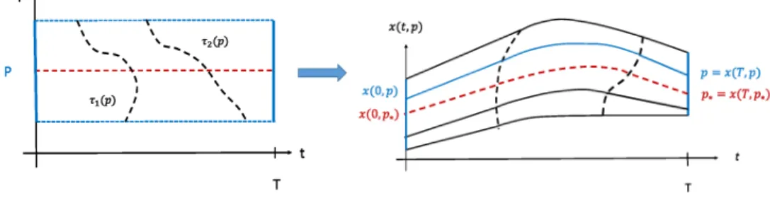
i.e., through the graphs of the corresponding trajectories. This is the correct formulation as our problem formulation overall is indeed time-dependent since there exists a fixed finite terminal time (e.g., see [14, pg. 324]). We emphasize that it is not required for a parameterized family of extremals that this flow defines an injective mapping. If it does, we call it afield of extremals. Obviously, since the trajectories for different parameter values typically obey different differential equations, it is quite possible that these graphs could intersect. In fact, conjugate points and associated loss of local optimality of extremals precisely correspond to fold singularities in this mapping while the reference controlled extremal will be a strong local minimum if this flow map is a diffeomorphism along the reference trajectory t 7→ x∗(t) = x(t, p∗) [14].
In principle, loss of injectivity of the flow can occur both in between the junction surfaces (and this corresponds to the classical conjugate points like in the calculus of variations) and at the junction surfaces (e.g., see [4, 11, 14]). In our case, however, since the controls remain continuous at junctions, the latter is not possible (also see [16]). Because of the continuity of the controls, trajectories before and after the junction point to the same side of the junction surface and thus the combined flow is injective near the junction surface (see Figure 2). In the terminology of [14], all junction surfaces aretransversal crossings. Hence, the strong local optimality of an extremal lift with regular junctions reduces to determiningwhether or not the flow map̥is a diffeomorphism along the reference controlled trajectory on the segments
between the junction times. If this is the case, then a continuously differentiable solution to the Hamilton-Jacobi-Bellman equation can be constructed on the region covered by the flow̥of extremals in the family by taking the cost along the extremals. The
desired strong local optimality of the reference trajectory then follows from classical results.
trajectories are solutions of the same differential equation and then this is merely the statement about uniqueness and smooth dependence on parameters for the solutions. It is the case when the controls lie in the interior of the control set that is the non-trivial one. However, in this case we are in the classical situation of neighboring feedback control laws (e.g., see [3, Chap. 6], [14, Sect. 5.3] or [16]). We briefly describe this theory and adjust its formulas to our problem formulation.
Fig. 2. A parameterized field of extremals with regular junctions
The mapping ̥: (t, p)→̥(t, p) = (t, x(t, p)) is a local diffeomorphism along the
reference trajectoryt→x(t, p∗) on the interval [ti, ti+1] if and only if the Jacobian
matrixD̥is nonsingular on the interval [ti, ti+1]. If we denote by ∂x∂p(t, p∗) then×n
matrix with (i, j) entry given by ∂xi
∂pj, i.e., the ith row is the gradient ofxi(t, p) with
respect to the parameter p, then this is equivalent to ∂x
∂p(t, p∗) being non-singular
on [ti, ti+1]. Note that this is automatic at the terminal timeT because of the chosen
parameterization,x(T, p)≡p, which gives ∂x∂p(T, p∗) =Id. Furthermore, ∂x∂p(t, p∗) is
non-singular over the interval [ti, ti+1] if and only if the matrix
S∗(t) =
∂λT ∂p (t, p∗)
∂x ∂p(t, p∗)
−1
(5.6)
is well defined over this interval. Similarly as above, the ith row of ∂λT
∂p is the the
gradient of λi(t, p) and the transpose is taken sinceλ is a row vector. The partial
derivatives ∂x
∂p(t, p) and ∂λT
∂p (t, p) are solutions of thevariational equations of (5.1)
and (5.2). Formally, these equations are obtained by differentiating equations (5.1) and (5.2) with respect to t and interchanging the partial derivatives with respect to p.
Using the relations
˙
x(t, p) =
∂H ∂λT(λ
T(t, p), x(t, p), u(t, p)
T
and
˙
λT(t, p) =
−∂H ∂x(λ
T(t, p), x(t, p), u(t, p)
it follows that (e.g., see [14, Sect. 5.3] and [16]) d dt ∂x ∂p
=HλTx ∂x
∂p+HλTu ∂u
∂p, (5.7)
and d dt ∂λT ∂p
=−HxλT ∂λT
∂p −Hxx ∂x ∂p −Hxu
∂u
∂p. (5.8)
Herex,u, λand their partial derivatives are evaluated at (t, p) and the second-order partial derivatives ofH are evaluated along the full extremals, (λ(t, p), x(t, p), u(t, p)). For notational clarity, however, we have dropped these arguments. Also, when differen-tiating the HamiltonianH twice with respect to column vectors (xorλT ), we write the corresponding matrices of second partial derivatives with the components of the first vector as row indices and the components of the second vector as column indices. Thus, the (i, j) entry of ∂x∂λ∂2HT is given by
∂2 H
∂xi∂λj. We denote this matrix by HxλT.
Note thatHλTx= (HxλT)T. Finally, we also have that HλTλT ≡0 sinceH is linear
in λ.
If the control uis constant on the domain Di ={(t, p) :τi(p)≤τi+1(p), p∈P},
then ∂u∂p(t, p)≡0 and we have that
d dt ∂x ∂p d dt ∂λT ∂p =
HλTx 0
−Hxx −HxλT
∂x ∂p ∂λT ∂p
. (5.9)
If the control utakes values in the interior of the control set on Di, then, by the maximum principle, we have that
∂H ∂u(λ
T(t, p), x(t, p), u(t, p))≡0.
Differentiating inp, it follows that
HuλT ∂λT
∂p +Hux ∂x ∂p +Huu
∂u
∂p ≡0. (5.10)
In our case,
∂2H
∂u2 =− 2
(1 +u)3hλ, g(x)i=− 2Φ
(1 +u)3 (5.11)
and this expression is positive if the control takes values in the interior of the control set (Theorem 3.1). Hence
∂u ∂p =H
−1
uu
Hux∂x
∂p +HuλT ∂λT
∂p
Substituting this expression into the variational equations gives the following homoge-neous matrix linear differential equation:
d dt ∂x ∂p d dt ∂λT ∂p =
HλTx−HλTuHuu−1Hux −HλTuHuu−1HuλT
−Hxx+HxuHuu−1Hux − HxλT −HxuHuu−1HuλT
∂x ∂p ∂λT ∂p . (5.13) Note that
HxλT −HxuHuu−1HuλT = HλTx−HλTuHuu−1Hux
T
.
Let X(t) = ∂x
∂p(t, p∗) andY(t) = ∂λT
∂p (t, p∗) be the solutions of the variational
equations along the reference extremal Γ∗. The variational equations are linear matrix
differential equations with time-varying coefficients given by continuous functions and thus these solutions exist on the full interval [ti, ti+1]. It is a classical result in control theory, going back to Legendre and the calculus of variations, that if a pair ofn×n
matrices (X, Y) is a solution to a linear matrix differential equation of the form
˙ X ˙ Y = A R
−M −AT X Y
, (5.14)
whereA,RandM are matrices whose entries are continuous functions over [ti, ti+1] and X(ti+1) is nonsingular, then the matrix X(t) is nonsingular over the interval
[ti, ti+1] if and only if there exists a solution to the matrix Riccati differential equation
˙
S+SA(t) +AT(t)S+SR(t)S+M(t)≡0, S(ti+1) =Y(ti+1)X(ti+1)−1 (5.15)
over the full interval [ti, ti+1] while the matrixX(τ) is singular if this Riccati differential
equation has a finite escape time τ ≥ ti. (For example, a proof is given in [14,
Proposition 2.4.1]). For an interior control we thus have the following result:
Proposition 5.3. Suppose the control u=u(t, p)takes values in the interior of the control set over the domainDi={(t, p) :τi(p)≤τi+1(p), p∈P}. If the matrix matrix X(ti+1) = ∂x
∂p(ti+1, p∗) is nonsingular, then X(t) = ∂x
∂p(t, p∗) is nonsingular on the full interval [ti, ti+1] if and only if there exists a solutionS∗ to the following matrix
Riccati differential equation (all partial derivatives are evaluated along the reference extremalΓ∗)
˙
S+S HλTx−HλTuHuu−1Hux
+ HλTx−HλTuHuu−1Hux
T
S (5.16)
−SHλTuHuu−1HuλTS+ Hxx−HxuHuu−1Hux≡0
with terminal condition S∗(ti+1) =Y(ti+1)X(ti+1)−1 over the full interval[ti, ti+1]. In this case, we have thatS∗(t) =Y(t)X(t)−1 for all t∈[ti, ti+1].
full interval. This once more confirms that the flow is a diffeomorphism along intervals where the reference control is constant, but, more importantly, gives us the formula for how to propagate the matrixS along those intervals. We summarize the statement in the proposition below:
Proposition 5.4. Suppose the control u=u(t, p)takes the constant valueu(t, p)≡0
oru(t, p)≡umax over the domainDi={(t, p) :τi(p)≤τi+1(p), p∈P}. If the matrix
X(ti+1) = ∂x
∂p(ti+1, p∗) is nonsingular, then X(t) = ∂x
∂p(t, p∗) is nonsingular over the full interval [ti, ti+1] and the matrixS∗(t) =Y(t)X(t)−1 can be computed as the
solution to the linear Lyapunov equation
˙
S+SHλTx+HxλTS+Hxx≡0 (5.17) with terminal conditionS∗(ti+1) =Y(ti+1)X(ti+1)−1.
Note that the Riccati differential equation (5.16) can be rewritten in the form ˙
S+SHλTx+HλTTxS+Hxx−(SHλTu+Hxu)Huu−1(HuλTS+Hux)≡0
which brings out its relation with the Lyapunov equation (5.17) more clearly. These equations only differ in the addition of a rank 1 matrix which accordingly is added respectively deleted as the reference control takes values in the interior of the control or goes back to boundary values. We therefore can combine Propositions 5.3 and 5.4 to obtain the following result (c.f., also [15, Sect. 4.1]):
Theorem 5.5. LetΓ∗= (x∗(·), u∗(·), λ∗(·))be an extremal lift with regular junctions
at timesti, i= 1, . . . , k, 0 =t0< t1<· · ·< tk< tk+1=T. LetS∗denote the solution
to the terminal value problem for the matrix Riccati differential equation
˙
S+SHλTx+HxλTS+Hxx−ι(SHλTu+Hxu)Huu−1(SHλTu++Hxu)T≡0, S∗(T) = 0,
(5.18)
where all partial derivatives are evaluated along the reference extremalΓ∗ andι= 1
on intervals where the control u∗ takes values in the interior of the control set and
ι= 0otherwise. If the solution S∗ exists on the full interval[0, T], then there exists
a neighborhood P ofx∗(T)such that the flow
̥: [0, T]×P→[0, T]×P, (t, p)7→(t, x(t, p)),
is a diffeomorphism on the domainD ={(t, p) : 0≤t≤T, p∈P}. In this case, the reference controlu∗ is a strong local minimum for problem[MM]. Specifically, the
refer-ence controlled trajectory(x∗, u∗)is optimal relative to any other controlled trajectory
(x, u)for which the graph of the trajectoryxlies in the set̥(D).
We still specify these formulas for model [MM]. Recall that
H =βx+γu+hλ, f(x) + u
1 +ug(x)i.
Hence
∂H
∂λ =f(x) + u
and thus
HλTx=Df(x) +
u
1 +u
Dg(x)
and
HλTu=
1
(1 +u)2g(x). Furthermore,
∂H ∂u =γ+
hλ, g(x)i
(1 +u)2 gives
Hux=
1
(1 +u)2λDg(x) and Huu=− 2
(1 +u)3hλ, g(x)i. In particular,
(SHλTu+Hxu)Huu−1(SHλTu++Hxu)T
=− 1
2(1 +u)hλ, g(x)i Sg(x) +Dg(x) TλT
Sg(x) +Dg(x)TλTT
.
Since the indicator function is negative when the control takes values in the interior, the matrix−(SHλTu+Hxu)Huu−1(SHλTu++Hxu)T is negative semi-definite and the
existence of a solution to the Riccati differential equation (5.18) is not guaranteed a priori by comparison results for solutions to Riccati differential equations. Indeed, this constitutes a true requirement for local optimality. In fact, it can also be shown that the existence of a solution on the interval (0, T] (open at the initial time) is a necessary condition for strong local optimality of the reference trajectory and thus these statements correspond to theJacobi conditionsin the calculus of variations.
6. CONCLUSION
In this paper we considered optimal control problems for the administration of one therapeutic agent when pharmacodynamics was modelled by a Michaelis-Menten relation, probably the most commonly used model in the pharmaceutical industry. It was shown that optimal controls are continuous concatenations of segments that consist of full or no dose controls connected by interior segments. This is in agreement with an interpretation of the controls as concentrations. Second-order conditions for local optimality of such extremals were formulated based on the method of characteristics in terms of the existence of a solution to a piecewise defined Riccati differential equation.
Acknowledgments
The research of U. Ledzewicz and H. Schättler is based upon work partially sup-ported by the National Science Foundation under collaborative research Grants Nos. DMS 1311729/1311733. Any opinions, findings, and conclusions or recommendations expressed in this material are those of the author(s) and do not necessarily reflect the views of the National Science Foundation.
REFERENCES
[1] B. Bonnard, M. Chyba, Singular Trajectories and their Role in Control Theory, Mathématiques & Applications, vol. 40, Springer Verlag, Paris, 2003.
[2] A. Bressan, B. Piccoli,Introduction to the Mathematical Theory of Control, American Institute of Mathematical Sciences, 2007.
[3] A.E. Bryson (Jr.), Y.C. Ho,Applied Optimal Control, Revised Printing, Hemisphere Publishing Company, New York, 1975.
[4] Z. Chen, J.B. Caillau, Y. Chitour,L1-minimization for mechanical systems, SIAM J. on Control and Optimization54(2016) 3, 1245–1265.
[5] M.M. Ferreira, U. Ledzewicz, M. do Rosario de Pinho, H. Schättler,A model for cancer chemotherapy with state space constraints, Nonlinear Anal.63(2005), 2591–2602. [6] P. Hahnfeldt, D. Panigrahy, J. Folkman, L. Hlatky,Tumor development under angiogenic
signaling: a dynamical theory of tumor growth, treatment response, and postvascular dormancy, Cancer Research59(1999), 4770–4775.
[7] A. Källén,Computational Pharmacokinetics, Chapman and Hall, CRC, London, 2007. [8] U. Ledzewicz, H. Schättler,Controlling a model for bone marrow dynamics in cancer
chemotherapy, Mathematical Biosciences and Engineering1(2004), 95–110.
[9] U. Ledzewicz, H. Schättler,The influence of PK/PD on the structure of optimal control in cancer chemotherapy models, Mathematical Biosciences and Engineering (MBE)2 (2005) 3, 561–578.
[10] P. Macheras, A. Iliadin,Modeling in Biopharmaceutics, Pharmacokinetics and Pharma-codynamics, Interdisciplinary Applied Mathematics, vol. 30, 2nd ed., Springer, New York, 2016.
[11] J. Noble, H. Schättler,Sufficient conditions for relative minima of broken extremals, J. Math. Anal. Appl.269(2002), 98–128.
[12] L.S. Pontryagin, V.G. Boltyanskii, R.V. Gamkrelidze, E.F. Mishchenko,The Mathe-matical Theory of Optimal Processes, Macmillan, New York, 1964.
[13] M. Rowland, T.N. Tozer,Clinical Pharmacokinetics and Pharmacodynamics, Wolters Kluwer Lippicott, Philadelphia, 1995.
[15] H. Schättler, U. Ledzewicz,Optimal Control for Mathematical Models of Cancer Thera-pies, Interdisciplinary Applied Mathematics, vol. 42, Springer, New York, 2015. [16] H. Schättler, U. Ledzewicz, H. Maurer,Sufficient conditions for strong locak optimality
in optimal control problems withL2-type objectives and control constraints, Dicrete and Continuous Dynamical Systems, Series B,19(2014) 8, 2657–2679.
[17] H.E. Skipper,On mathematical modeling of critical variables in cancer treatment (goals: better understanding of the past and better planning in the future), Bulletin of Mathe-matical Biology48(1986), 253–278.
[18] G.W. Swan,Role of optimal control in cancer chemotherapy, Mathematical Biosciences 101(1990), 237–284.
[19] A. Swierniak,Optimal treatment protocols in leukemia – modelling the proliferation cycle, Proc. of the 12th IMACS World Congress, Paris,4(1988), 170–172.
Maciej Leszczyński [email protected]
Lodz University of Technology Institute of Mathematics 90-924 Lodz, Poland
Elżbieta Ratajczyk [email protected]
Lodz University of Technology Institute of Mathematics 90-924 Lodz, Poland
Urszula Ledzewicz [email protected]
Lodz University of Technology Institute of Mathematics 90-924 Lodz, Poland
Southern Illinois University Edwardsville Department of Mathematics and Statistics Edwardsville, Il, 62026-1653, USA
Heinz Schättler [email protected]
Washington University
Department of Electrical and Systems Engineering St. Louis, Mo, 63130, USA