An empirically derived inorganic sea spray source function incorporating sea surface temperature

(1)

ACPD

15, 13783–13826, 2015

A sea spray source function incorporating SST

M. E. Salter et al.

Title Page

Abstract Introduction

Conclusions References

Tables Figures

◭ ◮

Back Close

Full Screen / Esc

Printer-friendly Version Interactive Discussion

Discussion

P

a

per

|

Discussion

P

a

per

|

Discussion

P

a

per

|

Discussion

P

a

per

|

Atmos. Chem. Phys. Discuss., 15, 13783–13826, 2015 www.atmos-chem-phys-discuss.net/15/13783/2015/ doi:10.5194/acpd-15-13783-2015

This discussion paper is/has been under review for the journal Atmospheric Chemistry and Physics (ACP). Please refer to the corresponding final paper in ACP if available.

An empirically derived inorganic sea

spray source function incorporating sea

surface temperature

M. E. Salter1, P. Zieger1, J. C. Acosta Navarro1, H. Grythe1,2,3, A. Kirkevåg4,

B. Rosati5, I. Riipinen1, and E. D. Nilsson1

1

Stockholm University, Department of Environmental Science and Analytical Chemistry, 11418 Stockholm, Sweden

2

Norwegian Institute for Air Research, P.O. Box 100, 2027 Kjeller, Norway

3

Finnish Meteorological Institute, Air Quality Research, Erik Palmenin aukio 1, P.O. Box 503, 00101 Helsinki, Finland

4

Norwegian Meteorological Institute, P.O. Box 43, Blindern, 0313 Oslo, Norway

5

Paul Scherrer Institute, Laboratory of Atmospheric Chemistry, 5232 Villigen, Switzerland

Received: 20 April 2015 – Accepted: 23 April 2015 – Published: 13 May 2015

Correspondence to: M. E. Salter (matthew.salter@aces.su.se)

(2)

ACPD

15, 13783–13826, 2015

M. E. Salter et al.

Title Page

Tables Figures

◭ ◮

Back Close

Full Screen / Esc

Discussion

P

a

per

|

Discussion

P

a

per

|

Discussion

P

a

per

|

Discussion

P

a

per

|

Abstract

We have developed an inorganic sea spray source function that is based upon state-of-the-art measurements of sea spray aerosol production using a temperature-controlled plunging jet sea spray aerosol chamber. The size-resolved particle production was measured between 0.01 and 10 µm dry diameter. Particle production decreased

non-5

linearly with increasing seawater temperature (between−1 and 30◦C) similar to

previ-ous findings. In addition, we observed that the particle effective radius as well as the

particle-surface, -volume and -mass, increased with increasing seawater temperature due to increased production of super-micron particles. By combining these measure-ments with the volume of air entrained by the plunging jet we have determined the

10

size-resolved particle flux as a function of air entrainment. Through the use of existing parameterisations of air entrainment as a function of wind speed we were subsequently able to scale our laboratory measurements of particle production to wind speed. By

scaling in this way we avoid the di_fficulties associated with defining the “white-area” of

the laboratory whitecap – a contentious issue when relating laboratory measurements

15

of particle production to oceanic whitecaps using the more frequently applied whitecap method.

The here-derived inorganic sea spray sea spray source function was implemented in a Lagrangian particle dispersion model (FLEXPART). An estimated annual global

flux of inorganic sea spray aerosol of 5.9_±0.2 Pg yr−1 was derived that is close to

20

the median of estimates from the same model using a wide range of existing sea spray source functions. When using the source function derived here, the model also showed

good skill in predicting measurements of Na+ concentration at a number of field sites

further underlining the validity of our source function.

In a final step, the sensitivity of a large-scale model (NorESM) to our new source

25

function was tested. Compared to the previously implemented parameterisation, a clear decrease of sea spray aerosol number flux and increase in aerosol residence time was observed, especially over the Southern Ocean. At the same time an increase in aerosol

(3)

ACPD

15, 13783–13826, 2015

M. E. Salter et al.

Title Page

Tables Figures

◭ ◮

Back Close

Full Screen / Esc

Discussion

P

a

per

|

Discussion

P

a

per

|

Discussion

P

a

per

|

Discussion

P

a

per

|

optical depth due to an increase in the number of particles with optically relevant sizes

was found. That there were noticeable regional di_fferences may have important

impli-cations for aerosol optical properties and number concentrations, subsequently also

affecting the indirect radiative forcing by non-sea spray anthropogenic aerosols.

1 Introduction

5

Primary marine aerosol or sea spray aerosol particles (SSA) are those particles pro-duced directly at the ocean surface following wave breaking, air entrainment as bub-bles, and the subsequent bubble bursting process at the ocean surface (Lewis and Schwartz, 2004). When considered in terms of mass, sea spray aerosol particles con-stitute the largest flux of particulate matter to the atmosphere after wind-blown dust,

10

with a global production of 3 to 30 Pg yr−1(Lewis and Schwartz, 2004).

Sea spray aerosol is important for the climate system where it acts as both a direct and indirect radiative forcing component (Stocker et al., 2013). Both of these forcing

e_ffects are highly dependent upon the total number and size distribution parameters of

the emitted sea spray aerosol particles; the direct effect is dominated by airborne

par-15

ticulate surface area while the indirect effect is more closely related to the number of

particles above a given size. Thus, sea spray aerosol properties have been the subject of significant scientific debate, centred on both the environmental factors that might

affect the production of sea spray aerosol and the best experimental approach to

esti-mate the source function of sea spray aerosol particles emitted (Lewis and Schwartz,

20

2004; de Leeuw et al., 2011).

Although wind speed is the major driver of air entrainment into surface waters, sim-ply parameterising sea spray aerosol production in terms of wind speed often fails to reconcile predicted and observed sea spray aerosol concentrations (e.g. Grythe et al., 2014). Secondary factors such as wave state and sea surface temperature (SST) are

25

known to affect a host of processes from initial air entrainment to the final production

(4)

ACPD

15, 13783–13826, 2015

M. E. Salter et al.

Title Page

Tables Figures

◭ ◮

Back Close

Full Screen / Esc

Discussion

P

a

per

|

Discussion

P

a

per

|

Discussion

P

a

per

|

Discussion

P

a

per

|

may also explain some of the disparity between different sea spray aerosol source

parameterisations (de Leeuw et al., 2011).

A number of recent findings have highlighted the potential importance of sea sur-face temperature on sea spray aerosol production. Salter et al. (2014) have shown that the interfacial bubble flux and bubble size spectra are strongly dependent on water

5

temperature and that these are strongly correlated to total particle number flux in a lab-oratory setting. Grythe et al. (2014) noted a strong influence of sea surface tempera-ture on sea spray aerosol production when they compared existing sea spray aerosol source functions with a global database of sea spray aerosol mass concentration

mea-surements. Salisbury et al. (2014) noted large differences between a commonly used

10

whitecap fraction parameterisation (Monahan and O’Muircheartaigh, 1980) derived al-most entirely in low-latitude regions and a satellite estimate derived over the entire globe. The authors postulate that the weaker wind speed dependence observed in their global dataset may in part be due to the influence of secondary factors which co-vary with the wind geographically, such as sea surface temperature. Their data

indi-15

cated that at a given wind speed, the satellite-derived whitecap fraction decreases with increasing sea surface temperature (see Fig. 9 in Salisbury et al., 2013).

Much of the discussion on the role of sea surface temperature in sea spray aerosol production has focused on the apparent contradiction between observations made us-ing laboratory systems that attempt to replicate oceanic whitecaps and observations

20

of sea salt concentrations made in the field or inferred from aerosol optical depth (AOD) measurements. A series of laboratory systems designed to replicate sea spray aerosol production by whitecaps have shown that the number production flux increases markedly as water temperatures are decreased (e.g. Salter et al., 2014; Zábori et al., 2013; Bowyer et al., 1990). In contrast, observational data from the field, such as

chem-25

ical analysis of particulate matter smaller than 10 µm (PM₁₀) or total suspended mass,

have often been used to infer that sea spray aerosol production increases with higher sea surface temperatures due to higher observed concentrations at lower latitudes (e.g. Jaeglé et al., 2011; Grythe et al., 2014). Similarly, Sofiev et al. (2011) noted a bias

(5)

ACPD

15, 13783–13826, 2015

M. E. Salter et al.

Title Page

Tables Figures

◭ ◮

Back Close

Full Screen / Esc

Discussion

P

a

per

|

Discussion

P

a

per

|

Discussion

P

a

per

|

Discussion

P

a

per

|

between predictions of sea spray aerosol induced aerosol optical depth and measure-ments of aerosol optical depth when using a sea spray source function not dependent on sea surface temperature. They noted that the aerosol optical depth determined near the tropics using a sea spray aerosol source function without sea surface temperature dependence was a factor of 2 lower than observations of aerosol optical depth,

sug-5

gesting that sea spray aerosol production was underestimated at lower latitudes where sea surface temperatures are higher and wind speed is generally lower.

One explanation for the aforementioned contradiction could be the distinct

proper-ties of the sea spray aerosol that the different approaches measure. In the laboratory

studies, emphasis has been placed on obtaining estimates of the number production

10

flux of particles. The majority of these studies have focused on particles smaller than 1 µm dry diameter, both through system design and instrumental restrictions, but also because this size range dominates sea spray aerosol number production. However, particles with dry diameter larger than 1 µm provide the dominant contribution to the fluxes of surface area and volume; thus, these particles are the most important for

ap-15

plications involving light scattering and particle mass. Consequently, studies that infer a temperature dependence of sea spray aerosol production fluxes based upon sea salt

concentrations (determined from PM₁₀ data) and aerosol optical depth measurements

in the field are likely to be highly influenced by the latter properties. The incongruity between laboratory studies and aerosol optical depth/sea salt mass studies may

sim-20

ply result from changes to the size distribution of sea spray aerosol coincident with changes to the total number production flux as seawater temperature changes.

To test this hypothesis we have determined the particle number flux in the size range

0.01 to 10 µm dry diameter (D_p) in a temperature-controlled laboratory sea spray

cham-ber. This setup previously highlighted a significant dependence of particle number

con-25

centration (Dp≥0.01 µm) on water temperature, with significant increases at lower

wa-ter temperatures (Salwa-ter et al., 2014). However, during these experiments this system

was not optimised to measure larger particles and suffered from significant particles

(6)

ACPD

15, 13783–13826, 2015

M. E. Salter et al.

Title Page

Tables Figures

◭ ◮

Back Close

Full Screen / Esc

Discussion

P

a

per

|

Discussion

P

a

per

|

Discussion

P

a

per

|

Discussion

P

a

per

|

measurements of PM₁₀, we have improved both the sampling protocol and the

instru-mentation used to measure particles withD_plarger than 1 µm (Sect. 3). Using this new

data we have derived a sea spray aerosol source function (Sect. 4) and compared it to field measurements using a Lagrangian particle dispersion model (FLEXPART; Stohl et al., 2005, see Sect. 5). Finally, we have deployed the new parameterisation in an

5

Earth system model (NorESM; Kirkevåg et al., 2013, see Sect. 6) to facilitate compari-son with the previous temperature dependent parameterisation.

2 Methods

2.1 The sea spray chamber

In order to observe the e_ffects of sea surface temperature on the source flux of aerosol

10

produced, we have utilised a temperature controlled sea spray generation chamber. This system has been described in detail by Salter et al. (2014). However, a number of modifications were made to the system to improve estimates of the aerosol particle

production flux, especially for particles withD_p>1 µm.

The sea spray chamber is fabricated from stainless steel components and

incorpo-15

rates temperature control (_±0.1◦C) so that the water temperature can be held constant

between−1 and 30◦C. Air was entrained using a plunging jet that exited a stainless

steel nozzle with inner diameter 4.3 mm held in a vertical position 30 cm above the air–water interface. Water was circulated from the centre of the bottom of the tank back through this nozzle using a peristaltic pump (Watson–Marlow, 620S) and silicone

20

tubing. All surfaces below the water level on the inside of the tank were coated in Teflon, and prior to all experiments all internal surfaces were rinsed thoroughly with reagent grade ethanol and low-organic-carbon (American Society for Testing and

Ma-terials Type 1) standard deionised water (>18.2 MΩ), hereafter referred to as DIW.

Both seawater salinity and temperature were measured continuously using an

Aan-25

deraa 4120 conductivity sensor. Seawater dissolved oxygen concentration was

(7)

ACPD

15, 13783–13826, 2015

M. E. Salter et al.

Title Page

Tables Figures

◭ ◮

Back Close

Full Screen / Esc

Discussion

P

a

per

|

Discussion

P

a

per

|

Discussion

P

a

per

|

Discussion

P

a

per

|

sured with an Aanderaa oxygen optode 4175. This sensor also provided an indepen-dent temperature measurement. Both sensors were placed towards the centre of the tank approximately halfway between the tank base and the air–water interface. Relative humidity and temperature were measured in the headspace of the sea spray simulator using a Vaisala model HMT333 probe.

5

Dry zero sweep air entered the tank at 6 L min−1 after passing through an ultrafilter

(Type H cartridge, MSA) and an activated carbon filter (Ultrafilter, AG-AK). The air-flow rate was maintained and quantified using a mass air-flow controller (Brooks, 5851S). Aerosol particle-laden air was sampled through a number of ports in the lid of the sea spray simulator and transferred under laminar flow to all aerosol instrumentation. To

10

prevent contamination by room air, the sea spray simulator was operated under slight

positive pressure by maintaining the sweep-air flow several L min−1 greater than the

sampling rate. Excess air was vented through a 1-way flutter valve on the lid of the system.

2.2 Particle size distribution measurements

15

2.2.1 Di_fferential mobility particle sizer and condensation particle counter

Aerosol particle-laden air was directed through 2 m of 1/4′′stainless steel tubing and

a custom made silica diffusion dryer at which point the flow was split. Immediately

fol-lowing this split a TSI model 3010 condensation particle counter (CPC) was used to

enumerate the total number concentration at 1 Hz for particles withD_p>0.01 µm. The

20

aerosol particle-laden air which entered the second sampling line was first directed

to a custom made impactor (0.0707 cm nozzle, with a cuto_ff diameter of _∼1 µm at

1 L min−1), it was then passed through a bipolar charger (neutralizer, Ni-63.), before it

entered a closed-loop sheath air, custom-built differential mobility particle sizer (DMPS)

which selected negatively charged particles using a positive high voltage in the di_ff

eren-25

tial mobility analyser (DMA). The selected particles were enumerated with a TSI 3772

(8)

ACPD

15, 13783–13826, 2015

M. E. Salter et al.

Title Page

Tables Figures

◭ ◮

Back Close

Full Screen / Esc

Discussion

P

a

per

|

Discussion

P

a

per

|

Discussion

P

a

per

|

Discussion

P

a

per

|

the size range 0.01 µm< Dp<0.7 µm (electrical mobility diameter) and a single scan

over 37 size bins was completed in 12 minutes.

A particle’s mobility equivalent diameter,D_mob, is defined as the diameter of a sphere

with the same electrical mobility as the particle.Dmobis only equal to the volume

equiv-alent diameter, D_ve, for spherical particles. Since NaCl and the other salts present in

5

the artificial seawater used during our study form cubic and not spherical particles when aerosolised and dried, we have shape corrected the mobility diameters obtained

using our DMPS. The relation betweenD_mobandD_veof a particle is:

f = Dve

D_mob =

1 χ

C_c(D_ve)

C_c(D_mob) (1)

wheref is the correction factor applied to each diameter measured, χ is the dynamic

10

shape factor of the particle, and C_c is the Cunningham slip correction factor (Hinds,

1999). For spherical particles,χ has by definition the value 1, while for NaClχ is equal

to 1.08 or that of a cube (Hinds, 1999). We assume that this value holds for the artificial sea salt used during our experiments and have used it to correct the size distributions obtained with our DMPS system to volume equivalent diameters.

15

2.2.2 White-light optical particle size spectrometer

Aerosol particle-laden air was vertically sampled and drawn directly upwards, without

bends or contractions in the sample line, through 0.75 m of 1/2′′stainless steel tubing

and a custom made silica diffusion dryer to a Palas WELAS 2300 white-light aerosol

spectrometer (WELAS; Palas GmbH) that was mounted directly above the sea spray

20

chamber. This is an optical particle size spectrometer (OPSS) with a white-light source

(Osram XBO-75 Xenon short arc lamp in the wavelength range of λ_≈350–750 nm)

that illuminates a measuring volume of_∼7 cm−3. Optical lenses collect the scattered

light between 78 and 102◦ with respect to the incident beam and direct it to a

pho-tomultiplier tube (PMT). The sensor is connected to the light source and detector via

25

(9)

ACPD

15, 13783–13826, 2015

M. E. Salter et al.

Title Page

Tables Figures

◭ ◮

Back Close

Full Screen / Esc

Discussion

P

a

per

|

Discussion

P

a

per

|

Discussion

P

a

per

|

Discussion

P

a

per

|

the sensor. This instrument was used to obtain the aerosol size distribution for the size

range 0.2 µm< D_p<10 µm (polystyrene latex sphere optical equivalent diameter) at

1 Hz, sizing particles in 59 bins.

Given that the OPSS instrument employs a white-light source it should be less in-fluenced by so called “Mie wiggles” than OPSS instruments which use monochromatic

5

light sources. Thus, the OPSS should be less affected by sizing ambiguities than a

sin-gle wavelength OPSS.

The OPSS reports equivalent optical diameters which were calculated by the in-strument’s firmware using a preset empirical calibration curve based on polystyrene latex (PSL) sphere measurements. In order to account for systematic instrumental

10

drifts caused by changes in the incident light intensity, changes of the PMT efficiency,

or degradations of the optical fibers, we made periodic measurements of 0.85 µm monodisperse Caldust (Calibration Dust provided by the manufacturer). Using these measurements the instruments firmware applied a correction factor to maintain a con-stant relation between scattered light intensity and optical diameter.

15

The probability that the OPSS will detect a particle is a function of the particle’s size

or cross section resulting in a size dependant counting efficiency. For particles close to

the small end of the OPSS sizing range there is a decreased probability of detection or

counting efficiency. Rosati et al. (2015) have determined the counting efficiency of the

OPSS used in this study and their results were similar to those of Mullins et al. (2012).

20

One hundred percent counting e_fficiency is attained for all particles larger than 0.3 µm,

and the counting efficiency increases to a maximum of∼130 %. The raw counts

ob-tained by the OPSS were multiplied by the reciprocal of the counting efficiency curve

generated by Rosati et al. (2015) to correct for the counting e_fficiency of the instrument.

As with all OPSS instruments, the OPSS measurements depend on the

wavelength-25

(10)

dif-ACPD

15, 13783–13826, 2015

M. E. Salter et al.

Title Page

Tables Figures

◭ ◮

Back Close

Full Screen / Esc

Discussion

P

a

per

|

Discussion

P

a

per

|

Discussion

P

a

per

|

Discussion

P

a

per

|

ferences in the refractive index of the materials. Since this diameter shift is likely to have a large influence on the aerosol particle surface and volume size distributions, we have corrected for it assuming that the sea salt aerosol particles had a refractive index

ofm=1.54₋0i (Abo Riziq et al., 2007) which corresponds to the value of NaCl

(com-pared to a refractive index ofm=1.588₋0i for the PSLs the instrument was calibrated

5

with).

As with the DMPS measurements, there is also an effect of particle shape on the

OPSS measurements. Therefore, these measurements were also corrected, through the use of PALAS PDAnalyze software, assuming that the shape factor of 1.08 for NaCl holds for the artificial sea salt used during these experiments.

10

2.2.3 Temperature and humidity of the sampled aerosol

The temperature and relative humidity (RH) of the sample entering the DMPS, as well as the sheath air of the DMPS were monitored using a Campbell Scientific HMP50 sensor. Although the relative humidity of the air entering the OPSS instrument was not measured directly, it is assumed that it was always well below 30 % such that the sea

15

spray aerosol had effloresced. This conclusion was made on the basis that all driers

were of identical design and because the flow through the OPSS drier was significantly

lower than the flow through the DMPS drier (OPSS: 0.5 L min−1; DMPS: 2 L min−1).

Based upon the dimensions of the diffusion driers used and the flow rates of the various

instruments, the residence time of the aerosol particle-laden air in the driers was _∼

20

6 s, and _∼1.5 s for the OPSS, and DMPS instruments respectively. The silica gel in

each drier was replaced when the relative humidity measured at the inlet to the DMPS exceeded 25 %. Therefore, we report our aerosol in dry diameters.

2.3 Experimental setup

Each experiment was conducted with artificial seawater (ASW) consisting of Sigma sea

25

salt (Sigma Aldrich, S9883; mass fraction: 55 % Cl−_{, 31 % Na}+_{, 8 % SO}2−

4 , 4 % Mg

2+_,

(11)

ACPD

15, 13783–13826, 2015

M. E. Salter et al.

Title Page

Tables Figures

◭ ◮

Back Close

Full Screen / Esc

Discussion

P

a

per

|

Discussion

P

a

per

|

Discussion

P

a

per

|

Discussion

P

a

per

|

1 % K+, 1 % Ca2+, <1 % other) rehydrated to an absolute salinity of 35 g Kg−1 _using

DIW. We subjected our artificial seawater to a purification process in the same manner as previously described by Salter et al. (2014). This consisted of activated charcoal

treatments, artificial UV exposures and hydrogen peroxide (H₂O₂, 30 % solution, no

stabilizer) additions. Here H₂O₂acted as an oxidising agent to remove organic matter.

5

Manipulating the water temperature in the sea spray chamber could potentially have changed gas saturation levels in the water. Since there has been speculation in the

liter-ature that sub- or super-saturations of atmospheric gases in seawater might affect

par-ticle production through changes to the bubble population (e.g. Stramska et al., 1990), we conducted constant temperature experiments to ensure that gas saturations were

10

in thermodynamic equilibrium with the headspace of the sea spray chamber. Once the artificial seawater purification procedure was complete, the water temperature was

held constant at a series of values between ₋1 and 30◦_{C whilst measurements of}

the aerosol generated were conducted. The water temperatures investigated were−1,

3, 5, 8, 10, 20, and 30◦C. At each water temperature aerosol measurements were

15

conducted over a period_≥2 h following a period of at least 12 h at the desired

tem-perature. Measurements of oxygen concentration in the seawater confirmed that gas saturations were in thermodynamic equilibrium and the oxygen % saturations were not

significantly di_fferent between the experiments. The mean oxygen saturation across

all experiments was 111 % with a standard deviation of 1 % (the reported accuracy of

20

the Aanderaa oxygen optode 4175 is to within<5 % saturation), within the range of

anomalies typically encountered in ocean surface waters (Najjar and Keeling, 1997). The second phase of the experiment consisted of measurements of the sea spray aerosol particles generated whilst the temperature of the water was slowly ramped

downward from 30 to 2◦C over a period of 29 h. This second phase was conducted

25

24 h after the first phase of experiments were completed. In the interim period the chamber was kept closed with a constant in-flow of zero-particle air and the same wa-ter was used for both experiments. At no point during the seawawa-ter cooling experiment

(12)

signifi-ACPD

15, 13783–13826, 2015

M. E. Salter et al.

Title Page

Tables Figures

◭ ◮

Back Close

Full Screen / Esc

Discussion

P

a

per

|

Discussion

P

a

per

|

Discussion

P

a

per

|

Discussion

P

a

per

|

cantly different than the mean of the constant temperature experiments (mean oxygen

saturation: 111 %).

2.4 Model simulations

2.4.1 The FLEXPART Lagrangian particle dispersion model

The FLEXPART Lagrangian particle dispersion model (Stohl et al., 2005) has been

5

used to simulate sea spray aerosol transport from its source to a series of observations

sites where chemical analysis of Na+ on aerosol filter samples has been conducted.

This model computes the trajectories of particles in the atmosphere to describe the

transport and turbulent diffusion of tracers. In this study particles were released from

the observation sites at a constant rate of 15000 particles per hour during every

mea-10

surement sampling interval and followed backwards in time for 20 days. When run in backward mode tracing mass concentrations the output of the model is an emission

sensitivity in seconds as a function of space (1◦_×1◦ with variable vertical resolution)

and time (every 3 h). By multiplying the emission sensitivity in the lowest model layer (100 m) by a source flux the source contribution is obtained which when integrated over

15

all grid cells and 3 hour intervals provides the simulated sea spray aerosol concentra-tion at the measurement point averaged over the sampling interval. Further detail on the manner in which we run this model can be found in Grythe et al. (2014).

In order to facilitate comparison with other commonly deployed sea spray source functions, four lognormal modes with modal diameters of 1.3, 9.4, 13.6, and 17.8 µm

20

and corresponding geometric standard deviations of 1.350, 1.100, 1.075, and 1.050 were used to approximate the source function presented in Sect. 4.

FLEXPART modelled sea spray aerosol concentrations using the parameterisation presented in this study are compared with the database of observed sea spray aerosol concentrations compiled by Grythe et al. (2014). This consists of observational data

25

obtained at 21 monitoring sites and on-board ships during 11 research cruises (see

(13)

ACPD

15, 13783–13826, 2015

M. E. Salter et al.

Title Page

Tables Figures

◭ ◮

Back Close

Full Screen / Esc

Discussion

P

a

per

|

Discussion

P

a

per

|

Discussion

P

a

per

|

Discussion

P

a

per

|

Table 1 in Grythe et al., 2014) and totals over 20000 observations distributed over the global oceans.

2.5 The NorESM Earth system model

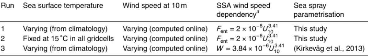
We have used a modified first version of the Norwegian Earth System Model, NorESM1-M (Bentsen et al., 2013; Iversen et al., 2013; Kirkevåg et al., 2013). This

5

model is run with intermediate atmospheric resolution (1.9◦_×2.5◦) and is based on the

CCSM4 model developed at NCAR (Gent et al., 2011). The model was set up to run in the same manner as described by Kirkevåg et al. (2013) with only slight modifications to the version of the atmospheric model, CAM4-Oslo. The model was set up using

pre-scribed sea surface temperatures and run in offline mode, so that changes in aerosol

10

treatment do not affect the meteorology.

The aerosol module in the atmospheric model, CAM4-Oslo, describes the size-resolved aerosol physics and transport of 20 aerosol components and combines a life-cycle model which handles the emissions, processing and transport of aerosol mass

combined with a physics scheme with look-up tables calculated by an o_ffline

micro-15

physics model. The look-up tables are used to compute the bulk (from size-resolved)

physical and optical properties of the aerosol population. The differences introduced

in the aerosol schemes compared to Kirkevåg et al. (2013) are the modified modal median diameters and standard deviations of the lognormal (and dry) sea spray size distributions at the point of emission. The new size parameters are listed in Table 1. The

20

(14)

ACPD

15, 13783–13826, 2015

M. E. Salter et al.

Title Page

Tables Figures

◭ ◮

Back Close

Full Screen / Esc

Discussion

P

a

per

|

Discussion

P

a

per

|

Discussion

P

a

per

|

Discussion

P

a

per

|

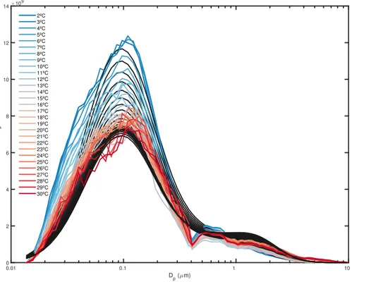
3 Results

3.1 Measured number size distributions during the constant temperature

experiments

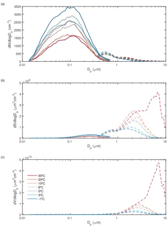
Over the 0.01 to 10 µm diameter size range covered by the DMPS system and OPSS

in-strument, when represented in the form dN/d logD_p, the size distributions obtained

dur-5

ing the constant water temperature experiments exhibit three modes (Fig. 1). A note-worthy observation is the apparent lack of agreement between the DMPS measure-ments and the OPSS measuremeasure-ments in the particle size range where they overlap. This is despite correcting both instruments for particle shape and correcting the OPSS instrument for the likely influence of particle refractive index. Both of these corrections

10

only influence the sizing of the particles and have no influence on the number of parti-cles counted by the instruments. Most likely the DMPS instrument was increasingly in-fluenced by particle losses due to the system tubing and the impactor placed before it in its upper sizing range. It should be borne in mind that the particle size range over which

the instruments disagree is not dominating dN/d logDp, dS/d logDpor dV/d logDpso it

15

is unlikely to influence the number fluxes, optical properties, or mass fluxes of the sea spray source function derived later in this study.

Following correction for the effect of shape, the DMPS system data exhibited a

sin-gle mode centred close to 0.1 µm when plotted in the form dN/d logD_p. This mode

decreased in number as the water temperature was increased between−1 and 30◦C.

20

Following correction for the effect of both shape and refractive index, the data obtained

using the OPSS exhibited two modes when plotted in the form dN/d logD_p. One was

centred around 0.55 µm and another was centred around 1.5 µm. The mode centred around 0.55 µm exhibited similar behaviour to the mode centred around 0.1 µm in that it decreased in number as the water temperature increased. However, the mode

cen-25

tred around 1.5 µm exhibited different behaviour in that it increased in number as the

water temperature was increased. This effect is much more prominent when the size

distribution is plotted in the form of the particle surface size distribution dS/d logD_p or

(15)

ACPD

15, 13783–13826, 2015

M. E. Salter et al.

Title Page

Tables Figures

◭ ◮

Back Close

Full Screen / Esc

Discussion

P

a

per

|

Discussion

P

a

per

|

Discussion

P

a

per

|

Discussion

P

a

per

|

particle volume size distribution dV/d logD_p which both assume that the particles are

spherical (Fig. 1).

Also noteworthy is the observation that the data obtained at 30◦C appears to show

a sudden shift in the size distribution to larger sizes. Although we cannot discount that

this effect is real, that we observe this effect only at a water temperature of 30◦C

sug-5

gests that this is more likely to have been a measurement artifact. Given that at a water

temperature of 30◦C in the chamber the air temperature was only slightly lower and the

sea spray chamber headspace had an RH of_∼98 %, the absolute water content will

have been high. This combined with the observed increase in the number of larger

particles (>1 µm) at this temperature relative to lower water temperatures may mean

10

that despite the fact that the RH at the inlet to the OPSS was below the e_fflorescence

point of the particles, assuming they were mainly NaCl, the particles may not have

had adequate time to fully effloresce and thus could have still been partially liquid. The

rate at which the particles were crystallising may also have changed, a factor which is

known to effect the ultimate shape NaCl particles take when dried (Wang et al., 2010).

15

3.2 Measured number size distributions during the temperature ramp

experiments

Once the constant temperature experiments were complete, an experiment where the

temperature of the water was slowly ramped downward from 30 to 2◦C over a period

of 29 h was conducted. In order to obtain estimates of the particle size distributions

20

as a function of water temperature during this experiment the data were binned at

a resolution of 1◦C. Here the data from the DMPS system and the OPSS have been

combined following corrections for particle shape and refractive index respectively. The two instruments both provide size resolved particle number in the dry diameter range

between∼0.2 to 0.7 µm. Given that for particles close to the small end of the OPSS

25

(16)

ACPD

15, 13783–13826, 2015

M. E. Salter et al.

Title Page

Tables Figures

◭ ◮

Back Close

Full Screen / Esc

Discussion

P

a

per

|

Discussion

P

a

per

|

Discussion

P

a

per

|

Discussion

P

a

per

|

the_∼1 µm impactor placed prior to it, we have chosen to use the DMPS measurements

in the range 0.01 to 0.45 µm and the OPSS measurements in the range 0.45 to 10 µm.

Measured dN/d logD_p was very similar to the constant temperature experiments,

consisting of three modes centred at dry diameters of _∼0.1, _∼0.55, and _∼1.5 µm

(see Supplement). The two smallest modes decreased in magnitude with increased

5

water temperature whilst the mode at the largest dry diameter exhibited opposite be-haviour and increased in number as the water temperature was increased. Once again this trend is much more apparent when the size distribution is presented in the forms

dS/d logD_pand dV/d logD_p. The sudden shift towards larger particles observed in the

constant temperature experiments was also apparent during the temperature ramp

ex-10

periments. However, it appeared at a slightly lower temperature of_∼23◦C.

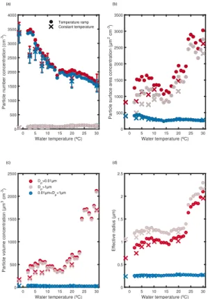
Comparison of the constant temperature experiments and the temperature ramp ex-periments is facilitated in Fig. 2. The integrated total particle number concentration (integrated across the size range 0.01 to 10 µm) in the temperature ramp experiments

was not significantly di_fferent to the constant temperature experiments. Figure 2d plots

15

the effective radius (r_e_ff) of both the constant temperature experiments and the

temper-ature ramp experiment as a function of water tempertemper-ature where:

r_e_ff=3V

A (2)

where V is the total integrated particle volume and A is the total integrated particle

surface area (assuming spherical particles). The effective radius of both the constant

20

temperature experiments and the temperature ramp experiment were also very similar at comparable water temperatures.

Given the observed similarity between the constant water temperature experiments and the water temperature ramp experiments as well as the higher water temperature resolution of the latter experiments, we have chosen to use the data from only the

25

temperature ramp experiments to generate a new inorganic sea spray aerosol param-eterisation as a function of water temperature in the following section.

(17)

ACPD

15, 13783–13826, 2015

M. E. Salter et al.

Title Page

Tables Figures

◭ ◮

Back Close

Full Screen / Esc

Discussion

P

a

per

|

Discussion

P

a

per

|

Discussion

P

a

per

|

Discussion

P

a

per

|

4 Derivation of a model parameterisation of the sea spray aerosol production

flux

4.1 Air entrainment as a function of wind speed

We have combined the number of particles in a unit logarithmic interval of D_p

pro-duced per unit time (p(D_p,T)) as a function of seawater temperature measured during

5

our experiments with measurements of the air entrained by the plunging jet as a func-tion of temperature presented in Salter et al. (2014). This approach is based on the assumption that all air entrained into the water column detrains as bubbles that pro-duce particles. Thus, the size-resolved particle production flux measured in the sea

spray chamber as a function of water temperature during our experiments (fτ(Dp,T)) is

10

defined as:

f_τ(D_p,T)=p(Dp,T)

τ(T) (3)

wherep(D_p,T) is the number of particles in a unit logarithmic interval of D_pproduced

per unit time as a function of water temperature (T) andτ(T) is the rate of air

entrain-ment in m3s−1_{as a function of water temperature.}

15

In order to estimate the size-resolved oceanic interfacial sea spray aerosol produc-tion flux, we have combined the size-resolved particle producproduc-tion flux from Eq. (3) with an estimate of the entrainment flux of air into the oceanic water column in the same manner as described by Long et al. (2011):

f_int(D_p,T)₌fτ(Dp,T)Fent (4)

20

whereF_entis the dependence of the air entrainment flux into the oceanic water column

on wind speed measured at 10 m height (U10).

As discussed by Long et al. (2011), the air entrainment flux into the water column

(F_ent) can be estimated from

F_ent=αǫ_d (5)

(18)

ACPD

15, 13783–13826, 2015

M. E. Salter et al.

Title Page

Tables Figures

◭ ◮

Back Close

Full Screen / Esc

Discussion

P

a

per

|

Discussion

P

a

per

|

Discussion

P

a

per

|

Discussion

P

a

per

|

whereǫ_dis the rate of energy dissipation by wave breaking in W m−2_and_α_{is the ratio}

of the volume of air entrained by breaking waves to the energy dissipated by the wind-wave through wind-wave breaking. As presented by Long et al. (2011), initially we assumed

a range of (4_±2)_×10−4_m3_J−1_for_α_{and that}_ǫ

dvaries as a function of wind speed as

(5_±1)_×10−5(U₁₀)3.74W m−2giving

5

F_ent=(2±1)×10−8

·(U₁₀)3.74 (6)

where F_ent is in m3m−2_s−1_{. However, this resulted in unrealistic over-production of}

sea spray aerosol at low latitudes in the Southern Hemisphere when implemented in the Earth system model, NorESM (see Sect. 6). Numerous existing sea spray aerosol parameterisations based upon the whitecap method utilise a wind speed dependence

10

of (U₁₀)3.41 with recent studies advocating even lower wind speed dependencies with

a smaller exponent forU10(e.g. Callaghan, 2013). Given this we have kept the scaling

to air entrainment the same as that used by Long et al. (2011) but use a lower wind

speed dependency of (U₁₀)3.41, which is the same value used by Kirkevåg et al. (2013).

This results in a final dependency of air entrainment on wind speed of

15

F_ent=2(_±1)_×10−8

·(U10)3.41 (7)

whereF_entis in m3m−2s−1.

4.2 E_ffective vs. interfacial sea spray aerosol fluxes

The aim of this study is to provide a parameterisation of sea spray aerosol production to represent the production flux in atmospheric chemical transport models or global

20

circulation models. Usually such models have their lowest atmospheric layer at 10 m and often much higher (e.g. 100 and 180 m in FLEXPART and NorESM, respectively). Therefore, knowledge of the size distribution of particles that attain significant height

in the atmosphere, often referred to as the effective flux, is required. Since the inlets

(19)

ACPD

15, 13783–13826, 2015

M. E. Salter et al.

Title Page

Tables Figures

◭ ◮

Back Close

Full Screen / Esc

Discussion

P

a

per

|

Discussion

P

a

per

|

Discussion

P

a

per

|

Discussion

P

a

per

|

to the aerosol instrumentation used during this study were sited ∼30 cm above the

water surface we have determined the flux of particles that reached this height, often

referred to as the interfacial flux. As such, consideration should be given to the di_ff

er-ence between the effective production flux and the interfacial production flux measured

at_∼30 cm.

5

Using an approach described by Lewis and Schwartz (2004) we have attempted to convert the interfacial fluxes measured in the sea spray chamber utilised during this

study to effective fluxes at 10 m height. This approach is outlined in detail in the

Sup-plement accompanying this work. Since the ratio of effective fluxes to interfacial fluxes

depends on both particle size and wind speed, computation of the e_ffective sea spray

10

aerosol particle flux should take into account both variables. However, since it would be

computationally expensive to compute the ratio of effective fluxes to interfacial fluxes

on the fly in Earth system models, we have converted the temperature dependent

in-terfacial fluxes measured during our study to temperature dependent effective fluxes

based upon a single wind speed (U₁₀) of 7 m s−1, approximately the global average

15

wind speed over the ocean. Although an implication of this assumption is that e_ffective

fluxes may be overestimated at wind speeds below 7 m s−1and underestimated at wind

speeds above 7 m s−1, we expect this effect to be negligible compared to the alternative

of simply implementing interfacial fluxes into models.

4.3 Size distribution as a function of temperature

20

Using the data presented in Sect. 3.2 we have generated a temperature dependent sea spray source function. Since the majority of Earth system models utilise modal mod-ules as input for aerosol emissions to limit computation time, we present our source function in this manner. A large number of these models are limited to three lognormal modes that are fixed to prescribed size-ranges with fixed model diameters and

geo-25

(20)

ACPD

15, 13783–13826, 2015

M. E. Salter et al.

Title Page

Tables Figures

◭ ◮

Back Close

Full Screen / Esc

Discussion

P

a

per

|

Discussion

P

a

per

|

Discussion

P

a

per

|

Discussion

P

a

per

|

The effective particle production flux (see Fig. 3) has been parameterized by fitting

the 1◦C binned interfacial number fluxes obtained during the temperature ramp

experi-ments corrected to an effective flux at 7 m s−1wind speed, to the sum of three lognormal

distributions of the form:

dF

d logD_p =

3

X

i=1

N_i

√

2πlogσ_i exp



−

1 2

logD_p−log ¯Dmod,i

2

logσ_i



 (8)

5

whereNi is the number production flux, ¯Dmod,i is the mode (median) diameter,σi is the

standard deviation of theith lognormal mode, and log is the logarithm with base 10.

Least-squares polynomial curve fitting was conducted to allow estimation of the

num-ber production flux (Ni) of the lognormal modes, with fixed modal diameters and

geo-metric standard deviations, as a function of water temperature. Therefore, in the final

10

form of the parameterisation, the number production flux (N_i) of each of the three

log-normal modes is a cubic function of sea surface temperature:

N_i=F_ent(_U₁₀₎_·(A_i_·T3+B_i_·T2+C_i_·T+D_i) (9)

whereF_ent(_U₁₀₎ is the volume of air entrained as a function ofU₁₀ (Eq. 7) and T is the

sea surface temperature in Celsius. Table 1 describes the details of the three modes

15

and the modal emission coe_fficients for use in Eq. (9).

Figure 3 depicts the number effective fluxes, per cubic metre of air entrained,

deter-mined from the temperature ramp data (see Sect. 3.2) using the approach described earlier in this section. Overlaid in black are the lognormal fits for each water tempera-ture obtained when the modal diameters and geometric standard deviations were fixed

20

to the values given in Table 1 and the number fluxes were estimated using the

polyno-mial coe_fficients given in Table 1 using Eq. (9). Generally the fits are able to account

for most of the variability in the measured number effective flux distributions, with the

coefficient of determination (R2) values of the fits ranging between 0.94 and 0.97 for

the effective number fluxes across the range of temperatures 2 to 30◦C. Comparison

25

(21)

ACPD

15, 13783–13826, 2015

M. E. Salter et al.

Title Page

Tables Figures

◭ ◮

Back Close

Full Screen / Esc

Discussion

P

a

per

|

Discussion

P

a

per

|

Discussion

P

a

per

|

Discussion

P

a

per

|

between the predicted surface area fluxes and those measured highlight

discrepan-cies, however. Between 2 and 22◦C the correlation between predicted surface area

fluxes and those measured is generally good withR2 values between 0.96 and 0.99.

However, at water temperatures higher than 22◦C the correlation between predicted

surface area fluxes and those measured becomes much poorer, withR2 values

de-5

creasing monotonically from 0.70 at 23◦C to 0.21 at 30◦C. This disconnect results

from the fact that the measured particles increase considerably in size, an effect which

the fits, constrained to constant modal diameter and geometric standard deviations, cannot account for. The observation that a transition to larger particle sizes occurred at

a water temperature of_∼23◦C was discussed in detail in Sect. 3.1 with the conclusion

10

that we cannot exclude that the particles had not fully effloresced at these higher water

temperatures. Given this, we have assumed that the small increase in the number of

super-micron particles observed as water temperatures increased from 2 to 22◦C

con-tinued at higher water temperatures by simply extrapolating the increase in the number production flux in the fitted mode centred at 1.5 µm observed in the water temperature

15

between 2 and 22 up to 30◦C.

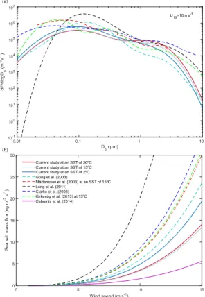
The source function estimated during this study is compared with a variety of

source functions from other recent studies for wind speeds of 10 m s−1 _{in panel a of}

Fig. 4 (Mårtensson et al., 2003; Gong, 2003; Long et al., 2011; Clarke et al., 2006) as well as the previous source function implemented in the Earth system model, NorESM

20

described by Kirkevåg et al. (2013). The latter source function is a slight modification of the previous sea spray aerosol treatment in NorESM1-M introduced by Struthers et al. (2013), which in turn was based on the Mårtensson et al. (2003) source func-tion. Therefore, it includes a dependence on sea surface temperatures. In contrast, the source functions of Gong (2003), Long et al. (2011) and Clarke et al. (2006) do not

in-25

(22)

ACPD

15, 13783–13826, 2015

M. E. Salter et al.

Title Page

Tables Figures

◭ ◮

Back Close

Full Screen / Esc

Discussion

P

a

per

|

Discussion

P

a

per

|

Discussion

P

a

per

|

Discussion

P

a

per

|

water temperature. All the source functions are shown for particle sizes normalised to dry diameter. The source function obtained during this study lies within the range of the other functions for all particle sizes measured.

Assuming the measured sea spray aerosol particles are spherical it is possible to integrate the sea spray aerosol mass flux to obtain mass emissions as a function of

5

wind speed and sea surface temperature. This can then be compared to observations as well as previously published sea spray aerosol source functions. Sea spray aerosol

mass emissions, ¯F can be obtained as follows:

¯

F =π

6ρss

Dp,2

Z

Dp,1

dF

d logD_pDp

3_d_D

p (10)

whereρ_ssis the density of sea salt, 2.16 g cm−3assuming it is similar to that of NaCl.

10

Panel b in Fig. 4 shows sub-micron ¯F (integrated across the size range: 0.029 µm<

D_p<0.580 µm) as a function of wind speed for the sea spray source function derived

during this study at sea surface temperatures of 2, 15, and 30◦C, a number of

pre-viously published source functions, the source function prepre-viously implemented in the Earth system model, NorESM described by Kirkevåg et al. (2013), as well as a fit to

15

measurements made at the Mace Head coastal station recently published by Ceburnis et al. (2014). It is clear from these figures that the previously published source func-tions, including the source function previously implemented in NorESM, overpredict

sub-micron sea salt mass emissions to the extent that atU₁₀=10 m s−1they are all at

least a factor of_∼3 too high. The Long et al. (2011) source function overpredicts by an

20

order of magnitude atU₁₀=10 m s−1in part due to its strong wind speed dependence

of (U₁₀)3.74. This appears to support our decision to reduce the wind speed

depen-dence of our function down from (U₁₀)3.74 to (U₁₀)3.41. Indeed, the new source function

presented in this study compares much better with the measurements of Ceburnis et al. (2014).

25

(23)

ACPD

15, 13783–13826, 2015

M. E. Salter et al.

Title Page

Tables Figures

◭ ◮

Back Close

Full Screen / Esc

Discussion

P

a

per

|

Discussion

P

a

per

|

Discussion

P

a

per

|

Discussion

P

a

per

|

5 Comparison to a Lagrangian particle dispersion model

Using European Centre for Medium-Range Weather Forecasts (ECMWF) wind fields over a 25 yr period, sea spray aerosol production was calculated using the source function presented here as well as a number of source functions more commonly de-ployed in large scale models. Annual mean global sea spray aerosol production was

5

5.9±0.2 Pg yr−1. Although this is at the low end of the range of estimates presented

by Grythe et al. (2014) of between 1.83 and 2444 Pg yr−1 it compares favourably with

the median of the 22 source functions of 5.91 Pg yr−1 _{(Grythe et al., 2014). For}

com-parison the source functions of Monahan et al. (1986), Gong (2003), and Sofiev et al.

(2011) produced 4.5, 4.6, and 2.6 Pg yr−1, respectively. Further comparison to existing

10

source functions can be made using Table 2 in Grythe et al. (2014).

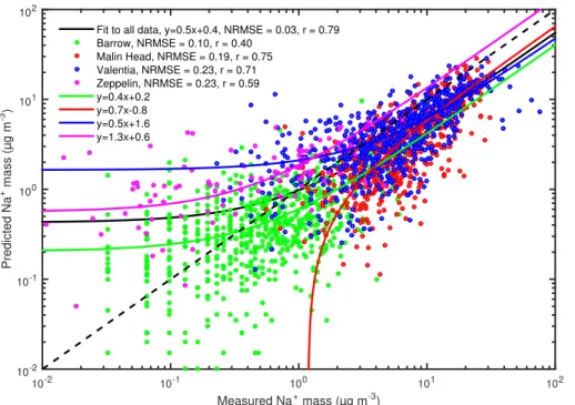
FLEXPART modelled sea spray aerosol concentrations using the parameterisation presented in this study can be compared with the database of observed sea spray aerosol concentrations compiled by Grythe et al. (2014). This consists of observa-tional data obtained at 21 monitoring sites and on-board ships during 11 research

15

cruises (see Table 1 in Grythe et al., 2014) and totals over 20000 observations dis-tributed over the global oceans. Figure 5 compares FLEXPART modelled with

mea-sured Na+ concentrations using the sea spray source function presented here for four

stations included in the comparison, Barrow, Malin Head, Valentia, and Zeppelin. The

Pearson’s correlation coe_fficient when comparing measured and modelled

concentra-20

tions at these four stations is 0.79 which compares favourably with those of other com-mon parameterisations when the same comparison was conducted by Grythe et al. (2014) of between 0.42 and 0.81. However, the performance of the model using the source function presented here ranged considerably across the four stations – lower skill was observed at the two polar stations, Barrow, Alaska, and Zeppelin, Svalbard,

25

which are characterised by lower concentrations of Na+ overall. Their distance from

(24)

representa-ACPD

15, 13783–13826, 2015

M. E. Salter et al.

Title Page

Tables Figures

◭ ◮

Back Close

Full Screen / Esc

Discussion

P

a

per

|

Discussion

P

a

per

|

Discussion

P

a

per

|

Discussion

P

a

per

|

tive of fresh sea spray aerosol. The Pearson’s correlation coefficient when comparing

the entire data set is 0.4, whilst it is 0.3, 0.8, and 0.3 when comparing only PM₁₀

measurements, EMEP station observations, and weekly observations, respectively. The value for the entire dataset compares favourably with the correlations between modelled and observed sea spray aerosol concentrations for other common sea spray

5

aerosol parameterisations found by Grythe et al. (2014). Here correlations ranged be-tween 0.16 and 0.41 when comparing the entire data set.

It is clear from Fig. 5 that the model is biased_∼50 % low compared to the

measure-ments. A low bias of similar magnitude was observed for many commonly deployed source functions tested by Grythe et al. (2014). It may be caused by the proximity of

10

the observations to coastal wave breaking in the form of surf which is not accounted for in the models, as well as inadequate treatment of sea spray aerosol post production in the model. For example, errors in the rate of below cloud aerosol scavenging in the

model will have knock-on effects on the aerosol residence time and how much of the

aerosol produced by wave breaking was predicted to reach the point of measurement.

15

6 Global simulations using an Earth system model

We ran a total of three two-year NorESM simulations after one year of spinup. The model was set-up as atmosphere-only and the atmosphere was coupled with the data ocean and sea-ice model (from CCSM4). In addition, the CAM4-Oslo aerosol life cycle

module was run o_ffline with respect to the atmospheric component so that the aerosol

20

changes induced by changing sea spray aerosol emissions in CAM4-Oslo had no effect

on the meteorology in any of the simulations. We chose not to include these feedbacks in order to obtain a clearer causal relation between sea surface temperature and sea spray aerosol given that all of these runs had exactly the same meteorology. All

sim-ulations employ emissions of SO₂, SO₄, particulate organic matter, and black carbon

25

from fossil-fuel and bio-fuel combustion and biomass burning, taken from the IPCC

(25)

ACPD

15, 13783–13826, 2015

M. E. Salter et al.

Title Page

Tables Figures

◭ ◮

Back Close

Full Screen / Esc

Discussion

P

a

per

|

Discussion

P

a

per

|

Discussion

P

a

per

|

Discussion

P

a

per

|

AR5 data sets as in Kirkevåg et al. (2013). The description of the runs and the sea spray parametrisation is presented in Table 2.

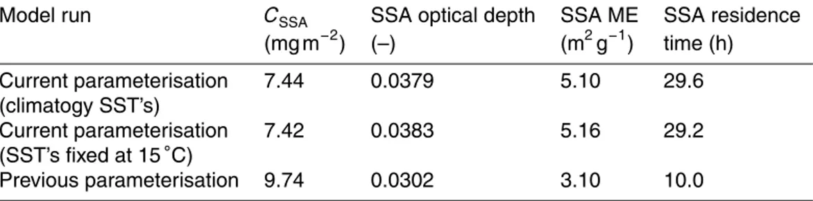
The global sea spray aerosol mass emission predicted by the model using the sea

spray source function presented in this study is 1.84_±0.92 Pg yr−1 _{whilst the global}

sea spray aerosol number emission is 210 000±105 000 particles m−2s−1 based on

5

the uncertainty in oceanic air entrainment presented by Long et al. (2011). Although the global sea spray aerosol mass emission predicted by NorESM is significantly lower than that predicted by the Lagrangian particle dispersion model, FLEXPART, the reader

should be aware that comparison between different model estimates is not direct. This

is because the di_fferent models have di_fferent assumptions for the sea spray size

rep-10

resentation. NorESM uses the three modes described in Table 1, whilst FLEXPART used four lognormal distributions with modal diameters of 1.3, 9.4, 13.6, and 17.8 µm and corresponding geometric standard deviations of 1.350, 1.100, 1.075, 1.050, re-spectively to approximate the source function (as well as all others in the comparison). To determine the influence of including a dependence on sea surface temperature in

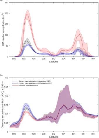
15

the sea spray aerosol source function relative to no dependence on sea surface

tem-perature we ran a simulation where the sea surface temtem-perature was fixed at 15◦C over

the entire ocean. Figure 6 plots the difference in sea spray aerosol number flux, mass

flux and clear-sky aerosol optical depth at 550 nm between the run with variable sea

surface temperatures and the run with sea surface temperatures fixed at 15◦C (the

20

variable sea surface temperature run minus the fixed sea surface temperature run). Sea spray aerosol number fluxes are slightly larger at higher latitudes in the North-ern Hemisphere and significantly larger at higher latitudes in the SouthNorth-ern Hemisphere

when a temperature dependence is included. There is no discernible difference at lower

latitudes in both hemispheres. When a temperature dependence is included, sea spray

25