Solar cycle signals in sea level pressure and sea surface temperature

(1)

ACPD

9, 25839–25852, 2009

Solar cycle signals in sea level pressure

and sea surface temperature

I. Roy and J. D. Haigh

Title Page

Abstract Introduction

Conclusions References

Tables Figures

◭ ◮

Back Close

Full Screen / Esc

Printer-friendly Version

Interactive Discussion Atmos. Chem. Phys. Discuss., 9, 25839–25852, 2009

www.atmos-chem-phys-discuss.net/9/25839/2009/ © Author(s) 2009. This work is distributed under the Creative Commons Attribution 3.0 License.

Atmospheric Chemistry and Physics Discussions

This discussion paper is/has been under review for the journal Atmospheric Chemistry and Physics (ACP). Please refer to the corresponding final paper in ACP if available.

Solar cycle signals in sea level pressure

and sea surface temperature

I. Roy and J. D. Haigh

Department of Physics, Imperial College, London, UK

Received: 29 October 2009 – Accepted: 20 November 2009 – Published: 2 December 2009 Correspondence to: I. Roy (i.roy06@imperial.ac.uk)

(2)

ACPD

9, 25839–25852, 2009

Title Page

Tables Figures

◭ ◮

Back Close

Full Screen / Esc

Interactive Discussion

Abstract

We identify solar cycle signals in 155 years of global sea level pressure (SLP) and sea surface temperature (SST) data using a multiple linear regression approach. In SLP we find in the North Pacific a statistically significant weakening of the Aleutian Low and a northward shift of the Hawaiian High in response to higher solar activity, confirming 5

the results of previous authors. We also find a weak but broad reduction in pressure across the equatorial Pacific. In SST we identify a weak El Ni ˜no-like pattern in the tropics, unlike the strong La Ni ˜na-like signal found recently by some other authors. We show that the latter have been influenced by the technique of compositing data from peak years of the sunspot cycle as these years have often coincided with the negative 10

phase of the ENSO cycle. Furthermore, the date of peak annual sunspot number generally falls a year or more in advance of the broader maximum of the 11-year solar cycle so that analyses which incorporate data from all years represent more coherently the difference between periods of high and low solar activity on these timescales.

1 Introduction

15

Signals of the 11-year solar cycle in various meteorological fields of the lower atmo-sphere, and in sea surface temperatures, have been presented by a number of authors. There is a consensus that any warming due to increased solar activity is not uniform, either within the atmosphere or at the ocean surface, but the patterns and amplitudes of the derived responses in temperature, and other fields, are still the subject of some 20

uncertainty. In sea level pressure (SLP) the Aleutian Low tends to be weaker when the Sun is more active and that the Hawaiian High moves northwards (Christoforou and Hameed, 1997). A large response is found in the Pacific in boreal winter: a positive anomaly in the Bay of Alaska, consistent with Christoforou and Hameed results, and also a reduction in SLP near the date line around 20–40◦N with a positive anomaly 25

(3)

ACPD

9, 25839–25852, 2009

Title Page

Tables Figures

◭ ◮

Back Close

Full Screen / Esc

Interactive Discussion This is consistent with the vL07 analysis of sea surface temperatures (SSTs) which

shows a strong La Ni ˜na (Cold Event, CE)-like signal when the Sun is more active. However, another SST analysis (White et al., 1997) shows a slightly warmer band of water across the tropical Pacific associated with peaks in a decadal signal (DSO) identified as in phase with solar activity. A modeling study suggests that coupling of 5

changes in surface windstress to ocean circulation produces a Warm Event (WE) a few years after solar maximum (Meehl and Arblaster, 2009) (MA09). It also suggests that the White et al results might be interpreted as lagging solar maximum by 1–2 years so that the results are not inconsistent. A more recent SST analysis (White and Liu, 2008), however, shows a phase-locking of harmonics of the ENSO time series with the 10

solar cycle resulting in a WE-like signal for about 3 years around the peak of the DSO (with CEs approximately 2 years either side of the peak, and stronger WEs peaking 3–4 years before and after it). Thus there is no clear picture of the SST response at solar maximum.

Any strong signal in SSTs would likely also be seen in near surface air temperature 15

but a multiple regression analysis of 118 years data (Lean and Rind, 2008) shows very little solar signal in the tropics. It does, however, show bands of warming around mid-latitudes in both hemispheres, consistent with a response seen previously in 27 years of zonal mean tropospheric air temperatures (Haigh, 2003). In this paper we investigate further the solar signal in SLP and SSTs using a multiple regression technique.

20

2 Data and methodology

We present results of a multiple linear regression analysis of over 150 years of SLP and SST data. For sea level pressures we use the Hadley Centre HadSLP2 dataset acquired from http://www.hadobs.org. This is an upgraded version of the monthly his-torical mean sea level pressure dataset HadSLP1, based on a compilation of numerous 25

(4)

ACPD

9, 25839–25852, 2009

Title Page

Tables Figures

◭ ◮

Back Close

Full Screen / Esc

Interactive Discussion We analyse two different sets of data for sea surface temperatures: one from the

Hadley Centre and another from NOAA. The Hadley Centre dataset (HadSST2), ob-tained from http://hadobs.metoffice.com/hadsst2/, is based on the recently created International Comprehensive Ocean Atmosphere Data Set (ICOADS) (Rayner et al., 2006). SST anomalies (relative to the mean values over 1961–1990) have been cal-5

culated over the globe between 1850 and 2004. The other SST dataset we use is the NOAA extended reconstructed sea surface temperature data set (ERSST.v2) for 1854– 2007 from http://www.cdc.noaa.gov/cdc/data.noaa.ersst.html. The two SST datasets differ in their data sources, in analysis procedure and the corrections algorithm applied before 1940s. In terms of sources, the NOAA product uses only in situ measurements 10

while Hadley centre data includes satellite-derived SST since early 1980s. The latter also includes additional in situ observations from the UK Meteorological Office archive which are not included in the former (Vecchi et al., 2007).

The independent time-varying indices we use in the multiple regression are a lin-ear trend (to simulate long-term climate change), stratospheric aerosol optical depth 15

(mainly representing the influence of explosive volcanic eruptions), solar variability and ENSO. We employ a code which estimates amplitudes of variability due to these cli-mate factors using an autoregressive noise model. In this methodology, noise co-efficients (that might be present due to several unobserved sources) are calculated simultaneously with the components of variability so that the residual is consistent with 20

a red noise model of order one. By this process it is possible to minimize noise being interpreted as signal. We then use a Student’s t-test to measure the level of confidence of variability for different indices.

Stratospheric aerosol optical depth data are from http://data.giss.nasa.gov/ modelforce/strataer/tau line.txt. It has been extended to 2005 with near zero values. 25

(5)

ACPD

9, 25839–25852, 2009

Title Page

Tables Figures

◭ ◮

Back Close

Full Screen / Esc

Interactive Discussion Thus we include solar variability on solar cycle timescales but do not include the effect

of any underlying long-term variations in solar irradiance which are di_fficult to separate statistically from a climate change signal.

3 Results

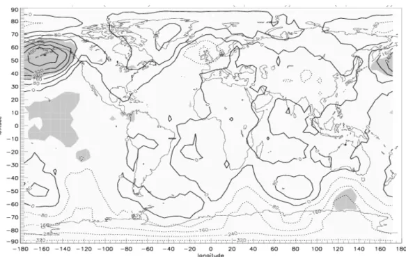
The signal in SLP associated by the multiple regression analysis with solar cycle vari-5

ability is presented in Fig. 1. It shows a region of positive anomaly, of up to 5 hPa, in the North Pacific with a smaller negative anomaly, magnitude around 0.5 hPa, in the equatorial Pacific. This pattern is robust to the inclusion or not of the ENSO index as an independent index in the regression analysis. It is consistent with the results of Christoforou and Hameed (1997) who showed that the Aleutian Low is weaker, and the 10

Hawaian High positioned further north, during periods of higher solar activity. It is also consistent with observational studies (Br ¨onnimann et al., 2006; Haigh et al., 2005) and modeling studies (Haigh, 1996, 1999; Larkin et al., 2000; Matthes et al., 2006) which have indicated an expansion of the zonal mean Hadley cell, and poleward shift of the Ferrel cell, at solar maxima. It does not, however, reproduce the pattern found by vL07, 15

using the HadSLP1 dataset, which placed a negative anomaly around 10–30◦_{N in the} mid-Pacific.

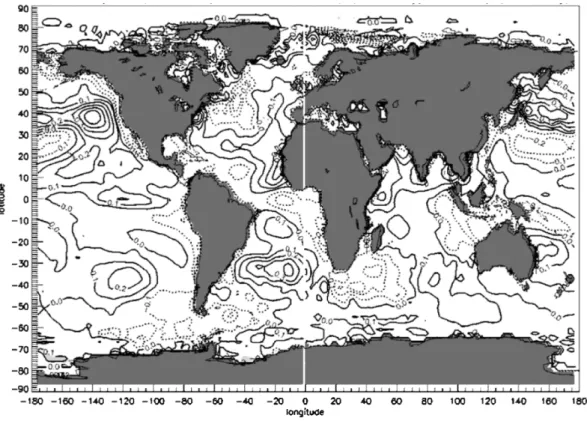
The solar cycle signal deduced in the NOAA SST data is presented in Fig. 2. No regions of high statistical significance are found but the pattern is essentially repro-duced using the HadSST2 dataset and is robust to the inclusion or otherwise of an 20

independent ENSO index. In the Eastern equatorial Pacific a tongue of warmer water is found, resembling a weak warm event. A stronger region of warming, of around 0.5K occurs at 40◦ latitude across the North Pacific, and more weakly in the South Pacific, with cooler regions equatorward in both hemispheres. The results in the North Pacific are qualitatively similar to those of vL07, although of much smaller magnitude, but in 25

(6)

ACPD

9, 25839–25852, 2009

Title Page

Tables Figures

◭ ◮

Back Close

Full Screen / Esc

Interactive Discussion and also the analyses of near surface air temperature by (Lean and Rind, 2008) and

(Haigh, 2003).

4 Discussion

To explain the apparent discrepancy between the di_fferent results, we investigate the different methodologies employed. vL07 deduced the solar signal by taking a com-5

posite of the data corresponding to the years identified with the peaks of the 14 solar activity cycles within the data period, and then associating the anomaly relative to the climatology with the effects of the Sun. The pattern was robust to the removal of data from either 1989 or 1905, the only years identified as having a strong ENSO influence. To investigate further any potential link between the apparent solar signal and ENSO 10

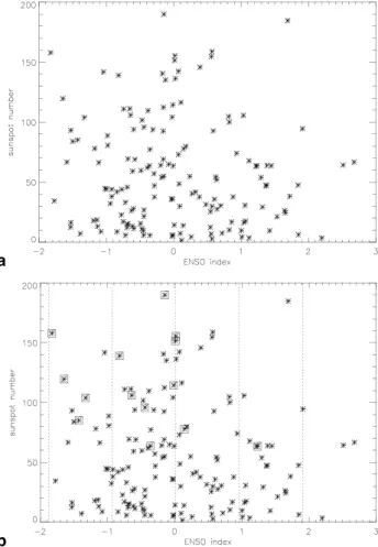
Fig. 3a presents a scatter plot of the values of these two parameters. No obvious relationship exists, and this is confirmed by a separate regression analysis of the ENSO time series (not shown). This would suggest that a signal identified with solar variability in tropical sea surface temperatures would be unlikely to express a particular phase of ENSO. When, however, solar cycle maximum years are identified, as shown in Fig. 3b, 15

nine of the fourteen have a value of ENSO index lower than the average, and four of these years (1893, 1917, 1989, 2000) are associated with particularly strong cold events. Only one solar maximum year is associated with a significant positive ENSO signal and this, 1905, is a weak solar cycle. As it is only the solar maximum years that are used by vL07 to characterize the solar signal it is clear that their result will resemble 20

a Cold Event (La Ni ˜na) pattern. It then remains to be determined to what extent the derived signal can be assigned as due to the Sun rather than mainly due to natural ENSO variability.

It is not immediately obvious why Fig. 2 should show a weak WE-like response as-sociated with higher sunspot numbers (SSNs) rather than the CE pattern of vL07, and 25

(7)

ACPD

9, 25839–25852, 2009

Title Page

Tables Figures

◭ ◮

Back Close

Full Screen / Esc

Interactive Discussion and Liu (2008) there is non-linear coupling between the two influences and that the

latter cannot be cleanly separated from the former. However, this cannot be the whole story as the solar signal produced by the regression is essentially unaffected by the in-clusion of an independent ENSO index and, furthermore, White and Liu (2008) show a WE pattern at the peak of the DSO with or without ENSO coupling. Rather, the answer 5

appears to be related to the definition of peak solar activity.

Figure 4 shows the time series of monthly SSNs and of their annual means, it also identifies the years of highest annual SSN for each solar cycle, as used by vL07 to label solar peak years. It is apparent that peak years tend to occur very soon after the solar cycle becomes more active – this is true of all the stronger cycles – and at least a 10

1 year before a date that would represent the peak of a broader decadal variation. Thus an analysis based on solar peak years, such as the vL07 results, represents the solar signal at a particular phase of the solar cycle while Fig. 2, and the results of White et al. (1997), represent more broadly the di_fference between periods of higher and lower SSN. The work of White and Liu (2008) provides an indication as to why these may not 15

give the same results as a WE signal near the peak of the DSO is typically preceded and followed, with a lead/lag of about 2 years, by a CE.

This difference in timing might also provide an explanation for other apparent discrep-ancies in solar signals. For example, in observational data van Loon et al. (2004) find a strengthening of the tropical Hadley cell when the Sun is more active while Kodera 20

and Shibata (2006) find it weakened. Peak sunspot number composites are used in the former paper while correlations between meteorological data and the 10.7 cm solar activity index are used in the latter and thus, from the arguments presented above, they represent different aspects of solar cycle variability. Similarly in modeling stud-ies: Meehl et al. (2008), with a transient model run analysed by peak SSN year, find 25

a stronger Hadley circulation while Haigh (1996, 1999), using equilibrated solar maxi-mum and minimaxi-mum experiments, finds a weaker Hadley cell.

(8)

ACPD

9, 25839–25852, 2009

Title Page

Tables Figures

◭ ◮

Back Close

Full Screen / Esc

Interactive Discussion solar response (Meehl and Arblaster, 2009) requires that changes in absorption of solar

radiation at the ocean surface initiate the earlier CE response. The processes involved would be akin to those proposed to be acting on centennial to millennial timescales, in which overall global warming increases meridional gradients in tropical sea surface temperatures, surface winds and shallow meridional overturning of the ocean (Clement 5

et al., 1996). Thus periods of higher insolation are statistically associated with an increased frequency of La Ni ˜na-like events (Mann et al., 2005). How the necessary changes in ocean circulation might become established within the timescale of the ascending portion of the solar cycle still needs to be established.

Given the small signals, and the availability of data covering only 14 solar cycles, it 10

remains a possibility that apparent solar cycles in tropical SSTs are produced by ran-dom statistical fluctuations. The signal in SLP, however, appears more robust. Studies with atmosphere-only models have shown that a significant mid-latitude response in temperature, wind and surface pressure can be induced by solar changes in the strato-sphere (Haigh, 1996, 1999). A more complete coupled atmostrato-sphere-ocean-chemistry 15

model study presents a similar tropospheric response to stratospheric solar forcing and suggests that this is responsible for more than half of the solar signal found in the troposphere (Rind et al., 2008).

5 Summary

We identify solar cycle signals in the North Pacific in 155 years of sea level pressure 20

and sea surface temperature data. In SLP we find in the North Pacific a weakening of the Aleutian Low and a northward shift of the Hawaiian High in response to higher solar activity, confirming the results of previous authors. We also find a broad reduction in pressure across the equatorial region but not the negative anomaly in the sub-tropics detected by vL07. Again, in SST we identify the warmer and cooler regions in the North 25

(9)

ACPD

9, 25839–25852, 2009

Title Page

Tables Figures

◭ ◮

Back Close

Full Screen / Esc

Interactive Discussion as that of vL07, based on composites of sunspot peak years find a La Ni ˜na response.

As the date of peak annual sunspot number generally falls a year or more in advance of the broader maximum of the 11-year solar cycle, analyses which incorporate data from all years represent more coherently the difference between periods of high and low solar activity on these timescales.

5

Acknowledgements. Indrani Roy is supported by a UK Natural Environment Research Council postgraduate studentship. We are grateful to Myles Allen for provision of the multiple regression code. The NERC British Atmospheric Data Centre provided access to some of the datasets.

References

Allan, R. and Ansell, T.: A new globally complete monthly historical gridded mean sea level

10

pressure dataset (HadSLP2): 1850–2004, J. Climate, 19(22), 5816–5842, 2006.

Br ¨onnimann, S., Ewen, T., Griesser, T., and Jenne, R.: Multidecadal signal of solar variability in the upper troposphere during the 20th century, Space Sci. Rev., 125(1–4), 3050–317, 2006. Christoforou, P. and Hameed, S.: Solar cycle and the Pacific “centers of action”, Geophys. Res.

Lett., 24(3), 293–296, 1997.

15

Clement, A. C., Seager, R., Cane, M. A., and Zebiak, S. E.: An ocean dynamical thermostat, J. Climate, 9(9), 2190–2196, 1996.

Haigh, J. D.: The impact of solar variability on climate, Science, 272(5264), 981–984, 1996. Haigh, J. D.: A GCM study of climate change in response to the 11-year solar cycle, Q. J. Roy.

Meteor. Soc., 125(555), 871–892, 1999.

20

Haigh, J. D.: The effects of solar variability on the Earth’s climate, Philos. T. R. Soc. A., 361(1802), 95–111, 2003.

Haigh, J. D., Blackburn, M., and Day, R.: The response of tropospheric circulation to perturba-tions in lower-stratospheric temperature, J. Climate, 18(17), 3672–3685, 2005.

Kodera, K. and K. Shibata.: Solar influence on the tropical stratosphere and troposphere in the

25

northern summer, Geophys. Res. Lett., 33(19), L19704, doi:10.1029/2006GL026659, 2006. Larkin, A. et al.: The e_ffect of solar UV irradiance variations on the Earth’s atmosphere, Space

Sci. Rev., 94(1–2), 199–214, 2000.

(10)

ACPD

9, 25839–25852, 2009

Title Page

Tables Figures

◭ ◮

Back Close

Full Screen / Esc

regional surface temperatures: 1889 to 2006, Geophys. Res. Lett., 35(18), L18701, doi:10.1029/2008GL034864, 2008.

Mann, M. E., Cane, M. A., Zebiak, S. E., and Clement, A.: Volcanic and solar forcing of the tropical Pacific over the past 1000 years, J. Climate, 18(3), 447–456, 2005.

Matthes, K. Kurodo, Y., Kodera, K., and Langematz, U.: Transfer of the solar signal from the

5

stratosphere to the troposphere: Northern winter, J. Geophys. Res.-Atmos., 111, D06108, doi:10.1029/2005JD006283, 2006.

Meehl, G. A., Arblaster, J. M., Branstator, G., and van Loon, H.: A coupled air-sea response mechanism to solar forcing in the Pacific region, J. Climate, 21(12), 2883–2897, 2008. Meehl, G. A., Brohan, P., Parker, D. E., and Folland, C. K., et al.: A Lagged Warm Event-Like

10

Response to Peaks in Solar Forcing in the Pacific Region, J. Climate., 22(13), 3647–3660, 2009.

Rayner, N. A., Lean, J., Lerner, J., Lonergan, P., and Leboissitier, A.: Improved analyses of changes and uncertainties in sea surface temperature measured in situ sice the mid-nineteenth century: The HadSST2 dataset, J. Climate, 19(3), 446–469, 2006.

15

Rind, D., Lean, J., Lerner, J., Lonergan, P., and Leboissitier, A.: Exploring the strato-spheric/tropospheric response to solar forcing, J. Geophys. Res.-Atmos., 113, D24103, doi:10.1029/2008JD010114, 2008.

van Loon, H. Meehl, G. A., and Arblaster, J. M.: A decadal solar effect in the tropics in July-August, J. Atmos. Sol. Terr. Phy., 66(18), 1767–1778, 2004.

20

van Loon, H., Meehl, G. A., and Shea, D. J.: Coupled air-sea response to solar forcing in the Pacific region during northern winter, J. Geophys. Res.-Atmos.,112(D2), 112, D02108, doi:10.1029/2006JD007378, 2007.

van Loon, H. and Meehl, G. A.: The response in the Pacific to the sun’s decadal peaks and con-trasts to cold events in the Southern Oscillation, J. Atmos. Sol.-Terr. Phy., 70(7), 1046–1055,

25

2008.

Vecchi, G. A. and Soden, B. J.: Global Warming and the Weakening of the Tropical Circulation, J. Climate., 20, 4316–4340, 2007.

White, W. B., Lean, J, Cayan, D. R., and Dettinger, M. D.: Response of global upper ocean temperature to changing solar irradiance, J. Geophys. Res.-Oceans, 102(C2), 3255–3266,

30

1997.

(11)

ACPD

9, 25839–25852, 2009

Title Page

Tables Figures

◭ ◮

Back Close

Full Screen / Esc

Fig. 1.The solar cycle signal in DJF sea level pressure (solar max – solar min, Pa). The solar

(12)

ACPD

9, 25839–25852, 2009

Title Page

Tables Figures

◭ ◮

Back Close

Full Screen / Esc

Fig. 2.The solar cycle signal in DJF sea surface temperature (solar max – solar min, K) using

(13)

ACPD

9, 25839–25852, 2009

Title Page

Tables Figures

◭ ◮

Back Close

Full Screen / Esc

Interactive Discussion a

b

Fig. 3. (a)Scatter plot of ENSO index against sunspot number, DJF values from 1856 to 2007

(14)

ACPD

9, 25839–25852, 2009

Title Page

Tables Figures

◭ ◮

Back Close

Full Screen / Esc

Fig. 4.Monthly mean sunspot number (thin curve) and the annual mean (thick curve). Vertical