ACPD
11, 23349–23419, 2011The Wildland Fire Emission Inventory
S. P. Urbanski et al.
Title Page
Abstract Introduction
Conclusions References
Tables Figures
◭ ◮
◭ ◮
Back Close
Full Screen / Esc
Printer-friendly Version Interactive Discussion
Discussion
P
a
per
|
Dis
cussion
P
a
per
|
Discussion
P
a
per
|
Discussio
n
P
a
per
|
Atmos. Chem. Phys. Discuss., 11, 23349–23419, 2011 www.atmos-chem-phys-discuss.net/11/23349/2011/ doi:10.5194/acpd-11-23349-2011
© Author(s) 2011. CC Attribution 3.0 License.
Atmospheric Chemistry and Physics Discussions
This discussion paper is/has been under review for the journal Atmospheric Chemistry and Physics (ACP). Please refer to the corresponding final paper in ACP if available.
The Wildland Fire Emission Inventory:
emission estimates and an evaluation of
uncertainty
S. P. Urbanski, W. M. Hao, and B. Nordgren
Missoula Fire Sciences Laboratory, Rocky Mountain Research Station, United States Forest Service, Missoula, Montana, USA
Received: 11 August 2011 – Accepted: 12 August 2011 – Published: 18 August 2011
Correspondence to: S. P. Urbanski ([email protected])
ACPD
11, 23349–23419, 2011The Wildland Fire Emission Inventory
S. P. Urbanski et al.
Title Page
Abstract Introduction
Conclusions References
Tables Figures
◭ ◮
◭ ◮
Back Close
Full Screen / Esc
Printer-friendly Version Interactive Discussion
Discussion
P
a
per
|
Dis
cussion
P
a
per
|
Discussion
P
a
per
|
Discussio
n
P
a
per
|
Abstract
We present the Wildland Fire Emission Inventory (WFEI), a high resolution model for non-agricultural open biomass burning (hereafter referred to as wildland fires) in the contiguous United States (CONUS). WFEI was used to estimate emissions of CO and PM2.5for the western United States from 2003–2008. The estimated annual CO
emit-5
ted ranged from 436 Gg yr−1 in 2004 to 3107 Gg yr−1 in 2007. The extremes in esti-mated annual PM2.5emitted were 65 Gg yr−1in 2004 and 454 Gg yr−1in 2007. Annual wildland fire emissions were significant compared to other emission sources in the western United States as estimated in a national emission inventory. In the peak fire year of 2007, fire emissions were∼20 % of total CO emissions and∼39 % of total PM2.5
10
emissions. During the months with the greatest fire activity, wildland fires accounted for the majority of CO and PM2.5emitted across the study region.
The uncertainty in the inventory estimates of CO and PM2.5 emissions (ECO and EPM2.5, respectively) have been quantified across spatial and temporal scales
rele-vant to regional and global modeling applications. The uncertainty in annual, domain
15
wide emissions was 28 % to 51 % for CO and 40 % to 65 % for PM2.5. Sensitivity of the uncertainty in ECO and EPM2.5 to the emission model components depended on
scale. At scales relevant to regional modeling applications (∆x=10 km, ∆t=1 day) WFEI estimates 50 % of total ECO with an uncertainty<133 % and half of total EPM2.5 with an uncertainty <146 %. The uncertainty in ECO and EPM2.5 is significantly
re-20
duced at the scale of global modeling applications (∆x=100 km, ∆t=30 day). Fifty percent of total emissions are estimated with an uncertainty<50 % for CO and<64 % for PM2.5. Uncertainty in the burned area drives the emission uncertainties at regional scales. At global scales the uncertainty in ECO is most sensitive to uncertainties in the fuel load consumed while the uncertainty in the emission factor for PM2.5 drives
25
ACPD
11, 23349–23419, 2011The Wildland Fire Emission Inventory
S. P. Urbanski et al.
Title Page
Abstract Introduction
Conclusions References
Tables Figures
◭ ◮
◭ ◮
Back Close
Full Screen / Esc
Printer-friendly Version Interactive Discussion
Discussion
P
a
per
|
Dis
cussion
P
a
per
|
Discussion
P
a
per
|
Discussio
n
P
a
per
|
modeling applications that employ the emission estimates. When feasible, biomass burning emission inventories should be evaluated and reported across the scales for which they are intended to be used.
1 Introduction
Biomass burning (BB; defined here as open biomass burning which includes wildfires
5
and managed fires in forests, savannas, grasslands, and shrublands, and agricultural fire such the burning of crop residue) is a significant source of global trace gases and particles (Ito and Penner, 2004; Michel et al., 2005; van der Werf et al., 2010). Biomass fire emissions comprise a substantial component of the total global source of carbon monoxide (40 %), carbonaceous aerosol (35 %), and nitrogen oxides (20 %)
(Lang-10
mann et al., 2009). Other primary BB emissions include greenhouse gases (CO2, CH4, N2O) and a vast array of photochemically reactive non-methane organic
com-pounds (NMOC; Akagi et al., 2011) that contribute to the production of ozone (O3) and
secondary organic aerosol (Pfister et al., 2008; Sudo and Akimoto, 2007; Alvarado et al., 2009).
15
Biomass burning emissions have a significant influence on the chemical composition of the atmosphere, air quality, and the climate system (Langmann et al., 2009; Lapina et al., 2006; Simpson et al., 2006). Fires influence climate through the production of long-lived greenhouse gases and short-lived climate forcers (e.g. aerosol) which are agents for direct and indirect (e.g. aerosols cloud effects) climate forcing. Biomass fires
20
contribute to air quality degradation by increasing the levels of pollutants that are detri-mental to human health and ecosystems, and that decrease visibility. The air quality impacts occur through the emission of primary pollutants (e.g. fine particulate mat-ter; PM2.5) and the production of secondary pollutants (e.g. O3and secondary organic
aerosol) when NMOC and nitrogen oxides released by biomass fires undergo
photo-25
ACPD
11, 23349–23419, 2011The Wildland Fire Emission Inventory
S. P. Urbanski et al.
Title Page
Abstract Introduction
Conclusions References
Tables Figures
◭ ◮
◭ ◮
Back Close
Full Screen / Esc
Printer-friendly Version Interactive Discussion
Discussion
P
a
per
|
Dis
cussion
P
a
per
|
Discussion
P
a
per
|
Discussio
n
P
a
per
|
al., 2004; Sapkota et al., 2005; Spracklen et al., 2007), and continental (Morris et al., 2006) scales.
BB emission inventories (EI) serve as critical input for Atmospheric Chemistry Trans-port Models (ACTM) that are used to understand the role of biomass fires in the at-mosphere and climate. BB EI are also important for interpreting in-situ and remote
5
atmospheric observations. The application determines the requirements of a specific BB EI, such as spatial and temporal resolution and chemical speciation. Modeling of regional air quality needs high resolution EI (∆x<∼25 km, ∆t≤1 day), while global
modeling applications can use less resolved input (∆x=0.5 to 3 degree,∆t=week to month).
10
Many BB emission models and inventories have been developed to provide input for a range of modeling applications. Case study EI have been assembled to assess the impact of specific fire events on air quality (e.g., the October 2003 wildfire outbreak in southern California, USA, Clinton et al., 2006; M ¨uhle et al., 2007; and prescribed burns in Georgia, Liu et al., 2009). Emission models to support the simulation of cumulative
15
smoke impacts from fires have been implemented for the contiguous United States (CONUS; Zhang et al., 2008; Larkin et al., 2009) and North America (Wiedinmyer et al., 2006). These models are designed to provide near-real-time fire emission estimates for air quality forecasts. Other region specific BB EI have covered boreal Siberia (1998– 2002; Soja et al., 2004), Africa (2000–2007; Liousse et al., 2010), and tropical Asia
20
(Chang and Song, 2010).
Several global BB EI have been produced in the last decade. The spatial and tem-poral resolution, speciation, and coverage period of the inventories varies consider-ably. Ito and Penner (2004) and Hoelzemann et al. (2004) published global, monthly EI for 2000 at spatial resolutions of 1 km and 0.5 degree, respectively. The Global Fire
25
contempo-ACPD
11, 23349–23419, 2011The Wildland Fire Emission Inventory
S. P. Urbanski et al.
Title Page
Abstract Introduction
Conclusions References
Tables Figures
◭ ◮
◭ ◮
Back Close
Full Screen / Esc
Printer-friendly Version Interactive Discussion
Discussion
P
a
per
|
Dis
cussion
P
a
per
|
Discussion
P
a
per
|
Discussio
n
P
a
per
|
rary inventory to reconstruct historical (1900–2000) emissions. The Fire Locating and Modeling of Burning Emissions (FLAMBE) program estimates near-real-time global BB emissions to support operational aerosol forecasting (Reid et al., 2009). The FLAMBE archive provides emissions datasets from 2000 to the present. The most recent ad-dition to global BB EI category was the Fire Inventory from NCAR (FINN), a global,
5
high resolution BB emission model that is capable of supporting near-real-time ap-plications (Wiedinmyer et al., 2011). A unique aspect of FINN is that it provides a comprehensive inventory of NMOC emissions allocated as lumped species for widely used atmospheric chemical mechanisms. FINN emission estimates are available for 2005–2010 with daily, 1 km resolution.
10
Agreement among the many BB EI is erratic. For example, GFED v3 and FINN v1 showed excellent agreement in annual, total CO2, CO, and CH4 emissions; over
2005–2009 the inventories agreed within 3–35 % for each compound (Wiedinmyer et al., 2011, van der Werf et al., 2010). In contrast, Stroppiana et al. (2010) compared five global BB EI (including GFED v3) for the year 2003 and found that total CO emissions
15
differed by a factor of 3.9 (high/low). The authors cited differences in the area affected by fires and vegetation characteristics as the prime causes for variability among inven-tories. On a continental basis, the disagreement in annual emission estimates among various inventories can be much greater. While 2003 total CO emissions for Africa varied by a factor of 2.2, those for North America varied by a factor of 14.5
(Stroppi-20
ana et al., 2010). Other inventories showed somewhat better agreement; for example, annual CO emissions estimated for North America by GFED v3 (van der Werf et al., 2010) and a continental BB EI (Wiedinmyer et al., 2006) differed by a factor of 1.15 to 1.93 over 2002–2004. Over shorter time periods, the disagreement between BB EI is more significant. Year 2003 monthly CO emissions for Africa from six different
25
ACPD
11, 23349–23419, 2011The Wildland Fire Emission Inventory
S. P. Urbanski et al.
Title Page
Abstract Introduction
Conclusions References
Tables Figures
◭ ◮
◭ ◮
Back Close
Full Screen / Esc
Printer-friendly Version Interactive Discussion
Discussion
P
a
per
|
Dis
cussion
P
a
per
|
Discussion
P
a
per
|
Discussio
n
P
a
per
|
contiguous United States (CONUS) varied by up to a factor of 10.
The disagreement among emission inventories and the lack of information regard-ing uncertainty at pertinent scales makes it difficult to determine which BB EI is most appropriate for a particular application and hinders the evaluation model results. For example, the annual, continental scale uncertainty reported for a BB EI may not be
5
applicable for an air quality simulation conducted with horizontal grid spacing of 10 km. This is particularly true given that BB emissions typically have large spatio-temporal gradients. Further, the sensitivity of the emission estimates to the model components is generally not well characterized. Understanding the sensitivity of emission estimates to assumptions and uncertainties associated with each input to the emission model –
10
burned area, fuel map, fuel load, fuel consumption, and emission factors, is crucial for properly assessing the impact these assumptions may have on ACTM simulations.
We present the Wildland Fire Emission Inventory (WFEI), a high resolution (500 m, 1 day) wildland fire emission model designed to support regional scale atmospheric chemistry studies and air quality forecasting. In this study, wildland fire refers to
non-15
agricultural, open biomass burning which differs from the more commonly used defini-tion of open BB which usually includes agricultural burning (e.g. pasture maintenance and crop residue). WFEI has been used to estimate emission of CO and PM2.5for the western United States from 2003–2008. We introduce a figure of merit, the half mass uncertainty, to evaluate uncertainty in the EI across spatio-temporal scales. The
spa-20
tial and temporal sensitivity of the WFEI estimates of CO and PM2.5 to uncertainties in mapped fuel loading, fuel consumption, burned area and emission factors is also examined. This may be the first study that has attempted to rigorously evaluate the uncertainties of a BB EI across a range of spatial and temporal scales. WFEI was de-signed for the contiguous United States and here it is applied to western United States
25
ACPD
11, 23349–23419, 2011The Wildland Fire Emission Inventory
S. P. Urbanski et al.
Title Page
Abstract Introduction
Conclusions References
Tables Figures
◭ ◮
◭ ◮
Back Close
Full Screen / Esc
Printer-friendly Version Interactive Discussion
Discussion
P
a
per
|
Dis
cussion
P
a
per
|
Discussion
P
a
per
|
Discussio
n
P
a
per
|
2 Methodology
2.1 Biomass burning emission model
Biomass burning emission (E) of a compound (i) is customarily estimated as the prod-uct of area burned (A; m2), fuel load consumed (FLC; kg-dry vegetation m−2), and specific emission factors (EF; kg-compoundi kg-dry vegetation−1) (Seiler and Crutzen,
5
1980):
E(k,t,i)=A(k,t)×FLC(k,t)×EF(k,t) (1)
In Eq. (1) FLC is the product of the fuel loading (FL; kg-dry vegetation m−2) and com-bustion completeness (C, dimensionless). All of the variables have significant spatial and temporal variability; in the above formulation k is the location (grid index) and t
10
is time. Equation (1) is the basis of WFEI which provides daily emission inventories with a spatial resolution of 500 m. WFEI was originally designed to provide near-real time wildland fire emissions for assimilation into air quality forecasting systems. The model combines observations from the MODerate Resolution Imaging Spectrora-diometer (MODIS) sensors on the Terra and Aqua satellites, meteorological analyses,
15
fuel loading maps, an emission factor database, and fuel condition and fuel consump-tion models to estimate emissions from wildland fires. The fire burned area is mapped using a MODIS-direct broadcast (DB) burn scar algorithm that combines active fire lo-cations and single satellite scene burn scar detections (Li et al., 2004). The MODIS-DB algorithm provides rapid mapping of burned area and enables production of a regional
20
emission inventory within 1 h of the final (Aqua), local MODIS overpass. We describe WFEI as applied to the western United States in the following sections.
2.1.1 MODIS based burned area
Burned area was mapped using an improved version of the MODIS-DB algorithm de-veloped by Urbanski et al. (2009a). Here we provide a brief overview of the algorithm
ACPD
11, 23349–23419, 2011The Wildland Fire Emission Inventory
S. P. Urbanski et al.
Title Page
Abstract Introduction
Conclusions References
Tables Figures
◭ ◮
◭ ◮
Back Close
Full Screen / Esc
Printer-friendly Version Interactive Discussion
Discussion
P
a
per
|
Dis
cussion
P
a
per
|
Discussion
P
a
per
|
Discussio
n
P
a
per
|
and describe the algorithm improvements and the MODIS data processed in this study. Details of the algorithm, a thorough evaluation of the algorithm, and a discussion of the deficiencies and limitations of burned area mapping using remote sensing and ground-based information are provided in Urbanski et al. (2009a) and references therein.
The MODIS algorithm combines active fire detections and single satellite scene burn
5
scar detections to map burned area with a nominal spatial and temporal resolution of 500 m and 1 day. While the algorithm was designed to process DB data in near-real-time, archived data may also be used. This study used MODIS Level-1B, Collection 5 Terra and Aqua datasets obtained from the NASA LAADS (NASA, 2011) to identify burn scars. Collection 5 of the standard MXD14 product (Giglio et al., 2003) provided
10
active fire detections (spatial resolution 1 km). The burn scar algorithm (Urbanski et al., 2009a) was applied to the Level-1B datasets to identify potentially burned pixels – pro-visional burn scar detections (spatial resolution 500 m). The purpose of the algorithm is to map wildland fire burned area; therefore the active fire and burn scar detections were filtered using an agricultural land mask (Sect. 2.1.2) to eliminate burning due to
15
agricultural activity. The processed data was aggregated temporally according to the date (Local Time) of satellite acquisition. Provisional burn scars were then screened for false detections using a contextual filter that eliminates pixels that are not proximate to a recent active fire detection. To be classified as ‘confirmed’, provisional burn scar detections were required to be within 3 km of any active fire detection from the
preced-20
ing 5 days. A daily burned area product was created by resampling the pixel centers of the confirmed burn scar detections onto a 500 m×500 m CONUS grid using a nearest neighbor approach. The burned area grid for each day was compared against a cumu-lative burned area grid which tracked the burned area for 90 days. Comparison against the cumulative burned area grid identified grid cells newly burned in the preceding day,
25
providing a map of burned area growth for that day.
ACPD
11, 23349–23419, 2011The Wildland Fire Emission Inventory
S. P. Urbanski et al.
Title Page
Abstract Introduction
Conclusions References
Tables Figures
◭ ◮
◭ ◮
Back Close
Full Screen / Esc
Printer-friendly Version Interactive Discussion
Discussion
P
a
per
|
Dis
cussion
P
a
per
|
Discussion
P
a
per
|
Discussio
n
P
a
per
|
versus 5 km and 10 days in the original. Second, in the current study, active fire detec-tions were used only to confirm burn scar detecdetec-tions. Previously, active fire detecdetec-tions were used to identify burned grid cells in addition to confirming burn scars. These improvements were proposed in Urbanski et al. (2009a) and their implementation has eliminated the overestimation of burned area in the original mapping scheme. An
eval-5
uation of the improved burned area mapping algorithm used in this study is provided in Appendix A.
2.1.2 Fuel map and fuel loading
The biomass, i.e. fuel loading (FL; kg dry vegetation m−2), subjected to fire in this study was estimated using wildland fuel loading models. A fuel loading model describes
10
and classifies fuelbed physical characteristics to provide numerical input for fire effects models (Sect. 2.1.4). In this study the fire effects models CONSUME (Prichard et al., 2006) and FOFEM (Reinhardt, 2003) were used to estimate the consumption of duff, litter, dead wood, herbaceous vegetation, and shrubs (Sect. 2.1.4). The Fuel Loading Models (FLM; Lutes et al., 2009) and the Fuel Characteristics Classification System
15
(FCCS; Ottmar, et al., 2007a) were the fuel loading models used in this study. We selected these fuel loading models because they have been mapped by the LANDFIRE project (LANDFIRE, 2011a, b) and they provide a full description of the dead wood and duff fuel strata that dominate loading, and hence potential emissions, in forested ecosystems of the western United States.
20
The FCCS is a tool to classify fuelbeds according to their potential fire behavior and fuel consumption (Ottmar et al., 2007a). The FCCS contains over 200 fuelbeds for the United States, organized according to vegetation type (e.g. Interior Ponderosa Pine – Douglas-fir Forest). The fuelbeds were developed using a wide range of sources: scientific literature, fuels photo series, fuel data sets, and expert opinion (Ottmar et al.,
25
2007a).
ACPD
11, 23349–23419, 2011The Wildland Fire Emission Inventory
S. P. Urbanski et al.
Title Page
Abstract Introduction
Conclusions References
Tables Figures
◭ ◮
◭ ◮
Back Close
Full Screen / Esc
Printer-friendly Version Interactive Discussion
Discussion
P
a
per
|
Dis
cussion
P
a
per
|
Discussion
P
a
per
|
Discussio
n
P
a
per
|
2009). The FLM were developed using an extensive database of surface fuel mea-surements from 4046 forested plots from across the contiguous United States. The FLM contains 21 fuel classes developed using a classification tree analysis to estimate the critical loads of duff, litter, fine woody debris, and coarse woody debris associated with 10 unique fire effects regimes. The 10 unique fire effects regimes were identified
5
by clustering the potential fire effects of each measurement plot as simulated using FOFEM (Lutes et al., 2009).
The major differences between the FCCS and FLM are:
1. The models were developed using different philosophies to classify fuelbeds; the FCCS fuelbeds are categorized according to vegetation type while the FLM
fu-10
elbeds are categorized based on the anticipated fire effects of the fuel loadings.
2. The FLM covers only forests, while the FCCS includes fuelbeds for herbaceous and shrubland cover types. The absence of FLMs for non-forest cover types re-quired the development of supplemental fuelbeds as part of our study (see below).
3. Due to a lack of data that satisfied their study’s criteria, the FLM provides only a
15
cursory treatment of understory herbs and shrubs. Because many of the plots in the FLM dataset (2707 of 4046) were missing herbaceous or shrub loadings, all of the FLM were assigned same loading, the dataset median, for these compo-nents. The FCCS provides specific herbaceous and shrub fuel loadings for each vegetation type classified.
20
4. The FLM were developed from a large, uniform collection of surface fuel mea-surements. In contrast, the FCCS were developed using a diverse range of data sources and the nature of the underlying data is variable across fuelbeds.
The original FLM classifies only forests and does not provide models for herbaceous or shrub fuelbeds that are important over large swaths of the western United States
25
ACPD
11, 23349–23419, 2011The Wildland Fire Emission Inventory
S. P. Urbanski et al.
Title Page
Abstract Introduction
Conclusions References
Tables Figures
◭ ◮
◭ ◮
Back Close
Full Screen / Esc
Printer-friendly Version Interactive Discussion
Discussion
P
a
per
|
Dis
cussion
P
a
per
|
Discussion
P
a
per
|
Discussio
n
P
a
per
|
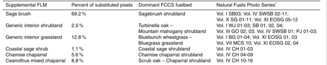
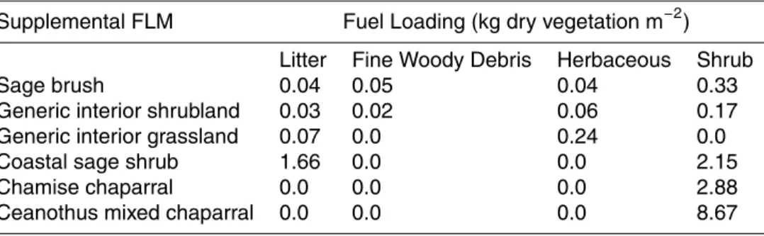
FLMs included these non-forested models. However, we chose not to use the Sikkink et al. (2009) fuel loads and instead opted to develop our own fuel loadings for non-forested classes of the LANDFIRE FLM map. Using the Natural Fuels Photo Series (Natural Fuels Photo Series, 2011) we developed six non-forest cover type fuel loading models: grass, sage brush, shrubs, coastal sage shrub, chamise, and ceanothus mixed
5
chaparral. We refer to these six fuel loading models as the “FLM supplemental models”. The photo series datasets and methods used to develop the FLM supplemental models are described in Appendix B.
Our study used the LANDFIRE FLM and FCCS spatial data layers (LANDFIRE, 2011b). The LANDFIRE spatial data layers are provided as 30 m resolution rasters
10
which we aggregated to 500 m resolution using majority resampling to match the reso-lution of our daily burned area product (Sect. 2.1.1). FLM and FCCS fuel codes were assigned to each burned grid cell by extracting the FLM and FCCS values from the 500 m rasters at the center point of each burned grid cell. Approximately 39 % of the fire im-pacted FLM pixels were non-forest and these FLM pixels were re-coded with the FCCS
15
codes of those pixels. The re-coded pixels were then assigned a FLM supplemental model based on the vegetation type of the FCCS fuelbed (Appendix B).
Our study did not include forest canopy fuels because the methods used in this study could not identify the occurrence of crown fire or reliably model canopy fuel consump-tion. While our burned area mapping technique efficiently identifies burned pixels, it
20
does not provide information regarding the occurrence of crown fire. The fuel con-sumption models used in this study (CONSUME and FOFEM) do not include empirical or physical process based modeling of canopy consumption. Additionally, the FLM do not include canopy fuel loading and augmentation of the FLM with canopy fuel load-ing estimates would have been problematic given the manner in which the FLMs were
25
ACPD
11, 23349–23419, 2011The Wildland Fire Emission Inventory
S. P. Urbanski et al.
Title Page
Abstract Introduction
Conclusions References
Tables Figures
◭ ◮
◭ ◮
Back Close
Full Screen / Esc
Printer-friendly Version Interactive Discussion
Discussion
P
a
per
|
Dis
cussion
P
a
per
|
Discussion
P
a
per
|
Discussio
n
P
a
per
|
2.1.3 Fuel conditions
Fuel moistures for dead and live fuels were calculated using the National Fire Danger Rating System (NFDRS) basic equations (Cohen and Deeming, 1985). The NFDRS provides fuel moisture models for live (woody shrubs and herbaceous plants) and dead fuels. Dead fuels are classified by timelag intervals (the e-folding time for a fuel
par-5
ticle’s moisture content to return to equilibrium with its local environment) which are proportional to the diameter of fuel particle (twig, branch, or log). The NFDRS clas-sifies 1-h, 10-h, 100-h, and 1000-h dead fuels corresponding to diameters of<0.64, 0.64–2.54, 2.54–7.62, >7.62 cm. 1-h and 10-h dead fuel moistures were calculated from the hourly air temperature (T), relative humidity (RH), and surface solar radiation
10
(SRAD) following the NFDRS implementation of Carlson et al. (2002). The meteo-rological input for the fuel moisture calculations was obtained from the North Amer-ican Regional Reanalysis (NARR) meteorological fields (32 km horizontal resolution, 45 vertical layers, and a 3 h output) (Mesinger et al., 2006). T, RH, and SRAD were estimated for the hours between analyses by interpolating the 3-hourly NARR output.
15
The NFDRS does not include equations for duff moisture, which is needed to predict duffconsumption and is required input for both CONSUME and FOFEM. The closed canopy empirical relationship of Harington (1982) was used to estimate the duff mois-ture from the NFDRS 100-h fuel moismois-ture. The Harrington (1982) study was limited to Ponderosa Pine forests and likely does not provide the best estimate of duffmoisture
20
for all forest ecosystem in the western UnitedStates. However, using the same methods to estimate fuel moistures for all cover types avoids introducing additional uncertain-ties into our analysis that would have interfered with our ability to assess uncertainuncertain-ties associated with the fuel consumption models, a key objective of this study.
2.1.4 Fuel consumption
25
meteoro-ACPD
11, 23349–23419, 2011The Wildland Fire Emission Inventory
S. P. Urbanski et al.
Title Page
Abstract Introduction
Conclusions References
Tables Figures
◭ ◮
◭ ◮
Back Close
Full Screen / Esc
Printer-friendly Version Interactive Discussion
Discussion
P
a
per
|
Dis
cussion
P
a
per
|
Discussion
P
a
per
|
Discussio
n
P
a
per
|
logical conditions (Rothermel, 1972; Albini, 1976; Anderson, 1983). Our study used two fire effects models, CONSUME and FOFEM, to simulate fuel consumption. While the models require similar input, fuel loading by fuel class (with slightly different size classifications for woody fuels) and fuel moisture, they employ significantly different ap-proaches towards predicting surface fuel consumption (dead wood and litter). While
5
both models were calibrated using field measurements of fuel consumption from wild-land fires, neither model has been extensively validated using independent data from wildfires or prescribed fires. Next we provide a brief description of the models.
CONSUME is an empirical fire effects model that predicts fuel consumption by fire phase (flaming, smoldering, residual smoldering), heat release, and pollutant
emis-10
sions (Prichard et al., 2006). The CONSUME natural fuels algorithms include pre-dictive equations for the consumption of shrubs, herbaceous vegetation, dead woody fuels, litter-lichen-moss, and duff. The dead woody fuels algorithms are comprised of equations for different size classes and decay status (sound or rotten). There are specific equations for dead wood and duffconsumption in the western United States.
15
Fuel moisture is the independent variable in all of the natural fuel equations except for the shrub, herbaceous vegetation, litter-lichen-moss, and 1-h size class dead wood (diameter<0.64 cm) strata.
FOFEM, the First Order Fire Effects Model, simulates fuel consumption, smoke emis-sions, mineral soil exposure, soil heating, and tree mortality (Reinhardt 2003). FOFEM
20
employs BURNUP (Albini et al., 1995), a physical model of heat transfer and burning rate, to calculate the consumption and heat release of dead woody fuels and litter. Duff consumption is calculated using the empirical equations of Brown et al. (1985). The consumption of herbaceous fuels and shrubs are estimated using rules of thumb (FOFEM 5.7, 2011). In addition to loading by fuel class, FOFEM requires fuel moisture
25
ACPD
11, 23349–23419, 2011The Wildland Fire Emission Inventory
S. P. Urbanski et al.
Title Page
Abstract Introduction
Conclusions References
Tables Figures
◭ ◮
◭ ◮
Back Close
Full Screen / Esc
Printer-friendly Version Interactive Discussion
Discussion
P
a
per
|
Dis
cussion
P
a
per
|
Discussion
P
a
per
|
Discussio
n
P
a
per
|
2.1.5 Emission factors
An emission factor (EF) provides the mass of a compound emitted per mass of dry fuel consumed. Our study developed “best estimate” CO and PM2.5 EFs for burning in forest and non-forest (grasslands and shrublands) cover types from data reported in the literature. The literature values used were fire-average EF measured for wildfires
5
and prescribed fires in the United States and southwestern Canada. The EF source studies were all based on in-situ emission measurements obtained from near source airborne or ground based tower measurements. The published EF were used to derive probability distribution functions (pdf) for EFCO and EFPM2.5that were used in our un-certainty analysis (Sect. 2.2.5). We used published EFs from 46 forest fires (Urbanski
10
et al., 2009b; Friedli et al., 2001; Yokelson et al.,1999; Nance et al., 1993; Radke et al., 1991) and 21 grassland/shrubland fires (Urbanski et al., 2009b; Hardy et al., 1996; Nance et al., 1993; Radke et al., 1991; Coffer et al., 1990) to derive pdf for EFCO. The pdf for EFPM2.5were obtained using EFs from 43 forest fires (Urbanski et al., 2009b;
Nance et al., 1993; Radke et al., 1991) and 17 grassland/shrubland fires (Urbanski et
15
al., 2009b; Hardy et al., 1996; Nance et al., 1993; Radke et al., 1991).
2.2 Evaluation of emission model uncertainty
2.2.1 Spatial and temporal aggregation
The emission model has a base resolution of 500 m and 1 day. The burned area is derived from the 24 h increase in burn scar, which is mapped once per day using the
20
combined MODIS data from the daytime overpasses of the Terra and Aqua satellites. In order to evaluate the dependence of the model’s uncertainty to scale, the base res-olution (500 m and 1 day) emission inventory was aggregated across multiple spatial grids (∆x=10, 25, 50, 100, 200 km) and time steps (∆t=1, 5, 10, 30, 365 day) provid-ing 25 arrays, g∆x,∆t(k,t). We use∆xand∆tto refer to the spatial and temporal scales
25
particu-ACPD
11, 23349–23419, 2011The Wildland Fire Emission Inventory
S. P. Urbanski et al.
Title Page
Abstract Introduction
Conclusions References
Tables Figures
◭ ◮
◭ ◮
Back Close
Full Screen / Esc
Printer-friendly Version Interactive Discussion
Discussion
P
a
per
|
Dis
cussion
P
a
per
|
Discussion
P
a
per
|
Discussio
n
P
a
per
|
lar spatio-temporal aggregation of the emission model: g25 km,30 day(k,t). “Elements” will be used to refer the array elements (k,t) of a particular spatio-temporal aggregate. The extent of the study’s spatial and temporal domains were the 11 western contiguous United States and from 1 January 2003 to 31 December 2008, respectively. The span of the spatial resolution was chosen to cover both regional (<∼25 km) and global (50 km
5
to 200 km) ACTM applications.
2.2.2 Monte Carlo analysis
The uncertainty of the emission model was estimated using a Monte Carlo analysis. The emission model is characterized by large uncertainties and non-normal distribu-tions. Monte Carlo analysis is a suitable approach for assessing the uncertainty of
10
such a model (IPCC, 2006) and has been applied in previous BB EI studies (French et al., 2004; van der Werf et al., 2010). In this paper we useσX, where X=A, FLC, or
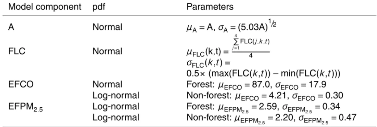
EF(i), to signify the 1-sigma (1σ) uncertainty of the model variables. The σX are the standard deviation of the model components used in the Monte Carlo analysis. The probability distribution functions (pdf) and parameters for A, FLC, and EF(i) are given
15
in Table 1. The approaches used to determine the pdf and parameters in Table 1 and their application in the Monte Carlo analysis are described in following sections. We useuX, whereX=A, FLC, EF(i), to refer to the 1σfractional uncertainty in estimated
value ofX,uX=σX/µX.
2.2.3 Burned area mapping uncertainty
20
MODIS vs. MTBS “ground truth”
We used burn severity and fire boundary geospatial data from the Monitoring Trends in Burn Severity (MTBS) project (MTBS, 2011a, b) to develop “ground truth” burned area maps to evaluate the uncertainty in our MODIS burned area product. MTBS is an ongoing project designed to consistently map the burn severity and perimeters
ACPD
11, 23349–23419, 2011The Wildland Fire Emission Inventory
S. P. Urbanski et al.
Title Page
Abstract Introduction
Conclusions References
Tables Figures
◭ ◮
◭ ◮
Back Close
Full Screen / Esc
Printer-friendly Version Interactive Discussion
Discussion
P
a
per
|
Dis
cussion
P
a
per
|
Discussion
P
a
per
|
Discussio
n
P
a
per
|
of large fire events (>404 ha) across the United States (MTBS, 2011c). The project uses LANDSAT TM/ETM images to identify fire perimeters and classify burn severity by 5 categories (1=unburned to low severity, 2=low severity, 3=moderate severity, 4=high severity, and 5=increased greenness). The fire severity classification is based on the differenced normalized burn ratio (dNBR) calculated from pre-fire and post-fire
5
LANDSAT images. MTBS analysts develop fire severity classifications from the dNBR for each individual fire event using raw pre-fire and post-fire imagery, plot data, and analyst experience with fire effects in a given ecosystem. We identified the annual “ground truth” burned area using the Regional MTBS Burn Severity Mosaic geospatial data (MTBS, 2011b). We mapped the “true” burned area from the MTBS dataset by
10
classifying all pixels with an MTBS severity class 2, 3, or 4 as burned.
The uncertainty assessment for our improved MODIS burned area mapping algo-rithm used data from several subregions representing the different land cover types of the western United States. The general approach was to aggregate the MODIS and MTBS burned pixels by the cells of a 25 km×25 km evaluation grid on an annual basis.
15
The MTBS project mapped only large fires (>404 ha), and while our MODIS burned area mapping algorithm was designed for large wildfire events, it does detect and map fire events<404 ha (Urbanski et al., 2009a). Therefore it is possible that our MODIS burned area mapping algorithm may accurately map small fire events that are not in-cluded in the MTBS dataset and that these MODIS detected burned pixels would
im-20
properly contribute to our assessment as false positive error. Therefore, we screened our MODIS data for burned pixels that were not associated with MTBS mapped fire events. MODIS active fire detections not within 3 km of an MTBS fire boundary (MTBS, 2011a) were flagged and the burn pixels confirmed by these active fire detections were excluded from the assessment. Even after spatial filtering, the screened MODIS burn
25
ac-ACPD
11, 23349–23419, 2011The Wildland Fire Emission Inventory
S. P. Urbanski et al.
Title Page
Abstract Introduction
Conclusions References
Tables Figures
◭ ◮
◭ ◮
Back Close
Full Screen / Esc
Printer-friendly Version Interactive Discussion
Discussion
P
a
per
|
Dis
cussion
P
a
per
|
Discussion
P
a
per
|
Discussio
n
P
a
per
|
tivity within each evaluation zone from the MTBS fire boundary data (MTBS, 2011a). Within each subregion (on an annual basis) we used the earliest reported start date from the MTBS perimeter data to identify the onset of wildfire activity. MODIS burned pixels in a particular evaluation zone which predated the beginning of wildfire activ-ity by more than 1 week were assumed to be prescribed fires and excluded from the
5
burned area assessment. Within each subregion, the filtered MODIS burned area and the MTBS based burned area were aggregated by the 25 km grid cells on an annual basis. The evaluation used data selected from 2005, 2006, and 2007, but in only a few cases was more than one year of data used in any subregion.
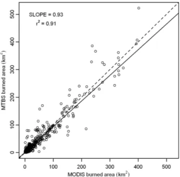
The MODIS burned area product was in close agreement with the MTBS burned
10
area (Fig. 1). The coefficient of determination was r2=0.91 and the Theil-Sen (TS) regression estimator indicated our MODIS burned area product slightly overestimated burned by 7 % (see Fig. 1). The TS regression estimator was selected over ordinary least squares regression because the burned area data in this study is non-normal distributed, heteroscedastic (the variance of the error term is not constant), and
con-15
tains high leverage outliers. The TS estimator is resistant to outliers and tends to yield accurate confidence intervals when data is heteroscedastic and/or non-normal in dis-tribution (Wilcox, 1998, 2005). The slope value of the TS estimator did not change when the intercept was forced to zero. The MODIS burned area was adjusted by the TS estimator slope (0.93) to correct for the slight overestimation. The MODIS burned
20
area used throughout the remainder of this paper is this adjusted MODIS burned area.
Uncertainty quantification
A primary goal of this study was to characterize the uncertainty in a biomass burning emission model, a task that requires uncertainty estimates for each model component. The burned area data has a non-normal distribution and is heteroscedastic. The
het-25
in-ACPD
11, 23349–23419, 2011The Wildland Fire Emission Inventory
S. P. Urbanski et al.
Title Page
Abstract Introduction
Conclusions References
Tables Figures
◭ ◮
◭ ◮
Back Close
Full Screen / Esc
Printer-friendly Version Interactive Discussion
Discussion
P
a
per
|
Dis
cussion
P
a
per
|
Discussion
P
a
per
|
Discussio
n
P
a
per
|
creases with increasing burned area (see Fig. 1). The default Breusch-Pagan test for linear forms of heteroscedasticity was used to formally verify the heteroscedastic condition of the dataset.
When data is non-normal in distribution and heteroscedastic, standard approaches for quantifying uncertainty are not reliable (Wilcox, 2005). Therefore, following Urbanski
5
et al. (2009a) and Giglio et al. (2010), we employed an empirical error estimation ap-proach to quantify the uncertainty of our MODIS based burned area measurement. The details of this analysis are provided in Appendix A and only the results are presented in this section. As evident in Fig. 1, and as demonstrated by Urbanski et al. (2009a), and by Giglio et al. (2010) (who used a more sophisticated MODIS burn scar mapping
10
technique) our analysis finds that the absolute uncertainty increases with increasing burned area. The 1σuncertainty in our MODIS mapped burned area is:
σA=(5.03×A) 1/2
(2)
where A is the MODIS measured burned area. While the absolute uncertainty (σA)
increases with burned area, the relative uncertainty (uA=σA/A) decreases. For
exam-15
ple, uA=71 % for a measured burned area of A=10 km2 and decreases to 22 % at A=100 km2. Uncertainty is typically expressed as an interval about a measurement result that is expected to encompass a specified probability range of the true value. In this study we defined the burned area uncertainty,uA, as the error cone expected
to contain approximately 68 % of the “ground truth” burned area values of which the
20
MODIS burned area is a measurement. This definition of uncertainty provides cov-erage comparable to that of a standard uncertainty for normally distributed data (i.e. coverage of∼68 % for 1σ). The empirical uncertainty analysis employed in this study (see Appendix A) satisfies our definition of uncertainty. Seventy two percent of the “ground truth” burned area values fall within the uncertainty bounds (Eq. 2) and when
25
ACPD
11, 23349–23419, 2011The Wildland Fire Emission Inventory
S. P. Urbanski et al.
Title Page
Abstract Introduction
Conclusions References
Tables Figures
◭ ◮
◭ ◮
Back Close
Full Screen / Esc
Printer-friendly Version Interactive Discussion
Discussion
P
a
per
|
Dis
cussion
P
a
per
|
Discussion
P
a
per
|
Discussio
n
P
a
per
|
2.2.4 Fuel load consumption uncertainty
The combination of fuel loading maps (FLM, FCCS) and consumption models (FOFEM, CONSUME) provided four predictions of fuel load consumption, FLC:
FLCi ,j=FLi×Cj (3)
where FL is the fuel loading (FL; kg-dry vegetation m−2), C is the consumption
com-5
pleteness, and FLC is the dry mass of vegetation consumed per m2. In Eq. (3) the i and j index identify the fuel loading model (FLM or FCCS) and fuel consumption model (FOFEM or CONSUME), respectively (FL1=FLM, FL2=FCCS, C1=FOFEM,
C2=CONSUME). At each element of the g∆x,∆t(k,t) we aggregated base resolution
FLC data (500 m and 1 day) and used the mean of the four predictions as the best
10
estimate of FLC (µFLC, Table 1). Sufficient observational data is not available to
eval-uate the estimates of FL, C or FLC; therefore, a statistical sample of the prediction error could not be used to quantify the uncertainty in the FLC. We made the subjective decision to estimate the uncertainty in the FLC predictions (σFLC, Table 1) as 50 % of
the range. Our uncertainty analysis does not account for mapping error, i.e. incorrect
15
assignment of fuel code in the LANDFIRE geospatial data. Mapping error could not be considered due to the absence of appropriate independent data.
2.2.5 Emission factor uncertainty
Published studies of over 50 fires in the United States and southwestern Canada (Sect. 2.1.5) were used to develop the forest and non-forest cover type pdf for EFCO
20
and EFPM2.5 in Table 1. The statistical variability of each EF (CO or PM2.5, forest or
non-forest) was determined by fitting log-normal and normal distributions to the source data. With the exception of EFCO for forest cover type, the EF were best described with a log-normal distribution. For each EF, the distribution model and fitted parame-ters (µand σ) were used in the Monte Carlo simulations (Sect. 2.2.2) to estimate the
ACPD
11, 23349–23419, 2011The Wildland Fire Emission Inventory
S. P. Urbanski et al.
Title Page
Abstract Introduction
Conclusions References
Tables Figures
◭ ◮
◭ ◮
Back Close
Full Screen / Esc
Printer-friendly Version Interactive Discussion
Discussion
P
a
per
|
Dis
cussion
P
a
per
|
Discussion
P
a
per
|
Discussio
n
P
a
per
|
uncertainty.µwas taken as the best estimate of EF. The pdf and parameters are given in Table 1.
2.2.6 Emission uncertainty
The Monte Carlo analysis provided an estimate of the model uncertainty for ECO and EPM2.5 by conducting 10 000 simulations at each of the 25 spatio-temporal
aggre-5
gates, g∆x,∆t(k,t). In each simulation round, possible CO and PM2.5 emission values
for each element were calculated using Eq. (1) where the values A, FLC, EF(i) were obtained by random sampling from each component’s pdf (Table 1). Both forest and non-forest EF values were drawn and the cover type weighted average of the two was used as the EF(i) at each element. The simulations provided 10 000 ECO and EPM25
10
estimates for each element of each g∆x,∆t(k,t), which served as the emission model pdf. The simulation results for ECO and EPM2.5were each sorted by increasing value and the 1σuncertainty bounds were taken as the 16th and 84th percentiles (elements Bl=1600 and Bu=8400 of the sorted simulation, respectively). Likewise, 90 % confi-dence intervals were taken as the 5th and 95th percentiles, Bl=500, Bu=9500. The
15
uncertainty bounds produced in this analysis are not symmetric due to truncation of negative values and the log-normal nature of EFPM2.5 and the EFCO for non-forest cover types (Table 1). When the uncertainty in the burned area was larger than the absolute burned area the lower uncertainty bound was truncated to 0. This truncation contributes to skewed uncertainty bounds for the emission estimates withσEX(upper)
20
>σEX(lower). The truncation effects associated with the burned area were most
preva-lent at small aggregation scales. The FLC pdf occasionally produced an uncertainty that was larger than µFLC resulting in a negative lower uncertainty bound which was
truncated to 0. Throughout the paper we use the larger, upper uncertainty bounds (84th or 95th percentiles) when referring to absolute or relative uncertainties. The
nomen-25
clatureσEX anduEX refers to the upper bound, 1σ absolute uncertainty and fractional
uncertainty in EX (uEX=σEX/EX), respectively. The best estimate of ECO and EPM2.5
ACPD
11, 23349–23419, 2011The Wildland Fire Emission Inventory
S. P. Urbanski et al.
Title Page
Abstract Introduction
Conclusions References
Tables Figures
◭ ◮
◭ ◮
Back Close
Full Screen / Esc
Printer-friendly Version Interactive Discussion
Discussion
P
a
per
|
Dis
cussion
P
a
per
|
Discussion
P
a
per
|
Discussio
n
P
a
per
|
that A (µAin Table 1), is simply the MODIS burned area measurement for each element
and that EF(i) is the cover type weighted average of the appropriateµfrom Table 1.
2.2.7 Variability and sensitivity of emission model uncertainty
In order to evaluate the uncertainty in our emission estimates across multiple scales we used a figure of merit, the half mass uncertainty, ˜uEX (where X=CO or PM2.5),
5
defined such that for a given aggregation level 50 % of total emissions (EX) occurred from elements withuEX <u˜EX. The figure of merit was calculated as follows: for each
g∆x,∆t(k,t), paireduEXand EX were sorted in order of ascendinguEXand the figure of
merit was taken as the value ofuEX where the cumulative sum of EX exceeded 50 %
of total EX. A graphical demonstration of ˜uEX is provided in Fig. S1. Thus, at a given
10
g∆x,∆t(k,t), 50 % of total ECO (EPM2.5) is estimated with an uncertainty less than ˜uECO
( ˜uEPM2.5).
We estimated the sensitivity of the uncertainty in our emission estimates to uncer-tainties in the model components using Eq. (4):
λEX,i=∂u˜EX
∂αi (4)
15
where σi is the uncertainty in one of the model components (i=A, FLC, EF). One
model component at a time, the 1σuncertainties from Table 1 were varied by a factor ofα=0.30 to 1.70 with an increment of 0.1. For each increment inα, the Monte Carlo analysis was repeated and the figure of merit, ˜uEX, was determined. Then the ˜uEX for
all α increments was regressed against α and the slope of this regression provided
20
ACPD
11, 23349–23419, 2011The Wildland Fire Emission Inventory
S. P. Urbanski et al.
Title Page
Abstract Introduction
Conclusions References
Tables Figures
◭ ◮
◭ ◮
Back Close
Full Screen / Esc
Printer-friendly Version Interactive Discussion
Discussion
P
a
per
|
Dis
cussion
P
a
per
|
Discussion
P
a
per
|
Discussio
n
P
a
per
|
3 Results
3.1 Emissions, burned area, and fuel consumption
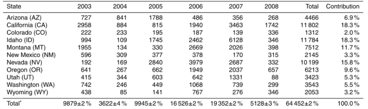
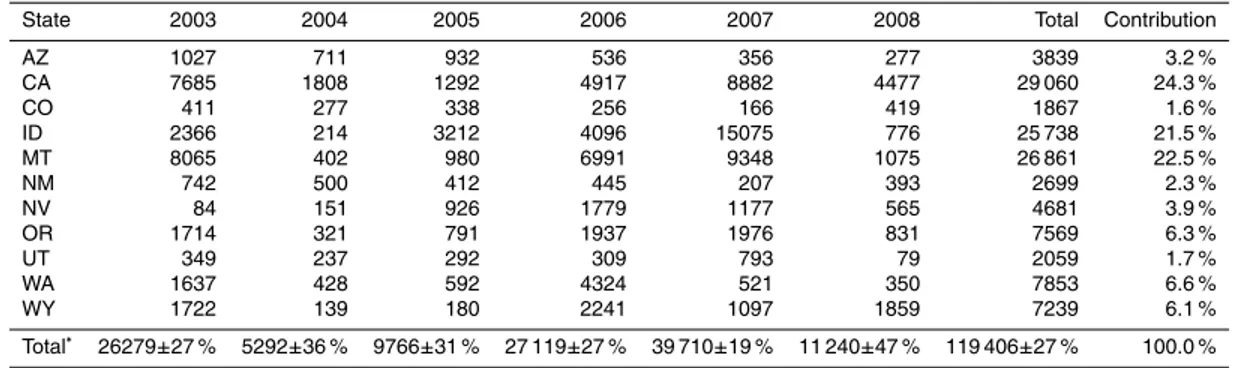
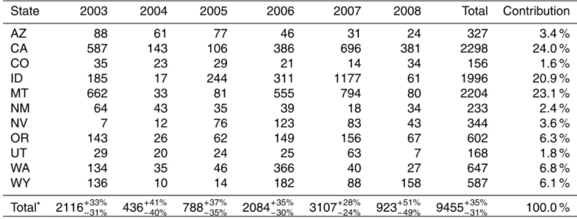
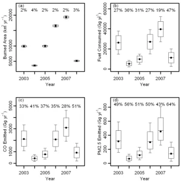
Annual burned area, fuel consumption (FC; FC=A×FLC), and emitted CO and PM2.5 for the western United States are shown in Fig. 2. The annual values and uncer-tainties were derived by annual aggregation of the base resolution (500 m and 1 day)
5
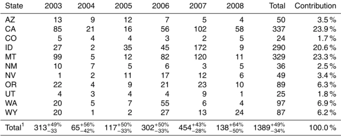
model components and emission estimates. The annual sums and uncertainties of A, FC, ECO, and EPM2.5 for each of the 11 states are provided in Tables 2 through
5. Maps of the annual burned area, fuel consumption, and emissions, aggregated to the∆x=25 km grid (i.e. g25 km,∆365 d(k,t)) are given in Figs. 3 through 6. There was significant inter-annual variability in the burned area, fuel consumption, and emissions.
10
The annual burned area ranged from 3622 to 19 352 km2. Fuel consumption was 5292 to 39 710 Gg dry vegetation yr−1. ECO was 436 to 3107 Gg yr−1and annual emissions of PM2.5 were 65 to 454 Gg. Burned area, fuel consumption, ECO, and EPM2.5 were all largest in 2007, and smallest in 2004; with 2007 emissions being∼7 times those in 2004. Burned area alone did not drive emissions. The significance of the ecosystems
15
involved in burning to fuel consumption and total emissions is easily seen by examining the years 2003, 2005, and 2006. In 2003 and 2005, the burned area was compara-ble, but fuel consumption, and thus emissions, were larger by a factor of∼2.7 in 2003. Similarly, despite a large difference in burned area between 2003 (9879 km2) and 2006 (16 526 km2), emissions of CO and PM2.5 differed by only a few percent. These diff
er-20
ences are not simply a function of the forested to non-forested burned area ratio, e.g. the fraction of forested burned area in 2003 and 2005 were roughly the same. And while in 2006 the fraction of burned area that was forest (49 %) was smallest of the six years, emission per area burned in 2006 exceeded that in 2004 and 2005 when 77 % and 68 % of burned area was forest, respectively.
25
ACPD
11, 23349–23419, 2011The Wildland Fire Emission Inventory
S. P. Urbanski et al.
Title Page
Abstract Introduction
Conclusions References
Tables Figures
◭ ◮
◭ ◮
Back Close
Full Screen / Esc
Printer-friendly Version Interactive Discussion
Discussion
P
a
per
|
Dis
cussion
P
a
per
|
Discussion
P
a
per
|
Discussio
n
P
a
per
|
and 6). Nearly half of the total estimated burned area over 2003–2008 occurred in three states: California (18.3 %), Idaho (18.3 %), and Montana (11.7 %). These three states accounted for two-thirds of estimated CO and PM2.5 emissions. Fire activity in Nevada comprised a large fraction of the total burned area (15.8 %), but owing to the sparse vegetation and light fuel loads of Nevada’s dominant ecosystems, ECO and
5
EPM2.5in this state were only a few percent of the total emissions.
During our study period, fire activity exhibited significant intra-annual variability. Burning was largely limited to June–October. More than 90 % of estimated burned area, fuel consumption, and emissions occurred during these months. This tempo-ral pattern is consistent with that of wildfire burned area reported in administrative
10
records covering 2000–2010 (National Interagency Coordination Center, 2011). The spatial distribution of monthly ECO during the fire season, summed over 2003–2008, is displayed in Fig. 7. Monthly burned area and ECO as percentages of the 2003– 2008 totals are also given in Fig. 7 (lower right panel). The maximum burned area occurred in July; however, emissions were a maximum in August due to the greater
15
fuel loadings involved. The seasonal fire activity originated in the southwest (Arizona, New Mexico, southern Nevada) in June. During July, fire activity expanded northward along the Rocky Mountains and through the Great Basin with the epicenter of activity migrating into northern Nevada and southern Idaho. Fire occurred throughout the in-terior west and Pacific Northwest over July. By August, fire activity had largely moved
20
into the northern Rocky Mountains and Pacific Northwest. Fire activity decreased in September and, outside of California, was minimal in October. In California, significant fire activity occurred in each month of the June–October period at some point over 2003–2008. October fires accounted for the largest monthly portion of burned area in California (36 %), followed by fires in July (19 %), September (13 %), August (12 %),
25
and June (9 %).
ACPD
11, 23349–23419, 2011The Wildland Fire Emission Inventory
S. P. Urbanski et al.
Title Page
Abstract Introduction
Conclusions References
Tables Figures
◭ ◮
◭ ◮
Back Close
Full Screen / Esc
Printer-friendly Version Interactive Discussion
Discussion
P
a
per
|
Dis
cussion
P
a
per
|
Discussion
P
a
per
|
Discussio
n
P
a
per
|
bin. From Fig. 8 it is readily apparent that a small fraction of elements were responsible for the majority of total emissions. At g25 km,30 d(k,t) 83 % of total ECO originated from 10 % of elements and a mere 2.5 % of elements were responsible for over half of total ECO (56 %). The pattern is similar, though not as extreme, at g10 km,1 d(k,t), 64 % of total ECO arose from 10 % of the elements and 36 % of total ECO occurred in 2.5 %
5
elements. This result is consistent with previous findings which found that very large wildfires (burned area>100 km2) accounted for a substantial portion of burned area in the western United States (Urbanski et al., 2009a). The large spike at bin=3.8 stems from quantization effects. The burned area of the elements in this bin are mostly at the minimum detection level (500 m) and are dominated by two fuel types which have
10
nearly identical fuel loadings. The difference in fuel load (which sets the upper limit on emissions) between the two fuel types is less than the resolution of the frequency bins (1.25 kg).
3.2 Uncertainty
3.2.1 Annual domain wide
15
The uncertainty in the estimated annual burned area was≤5 % (Fig. 2a). Due to the large burned area for annual, domain wide aggregation, the lower bound uncertainties were never negative and were not truncated. In this absence of truncation effects, the uncertainty bounds are symmetric. The uncertainties in ECO were slightly skewed to-wards the upper bounds which ranged from 28 % to 51 % (Fig. 2c). The asymmetry
20
in theuECO reflects the tail of the log-normal distribution for EFCO in non-forest fuels
(Sect. 2.2.3). The uncertainty in estimated EPM2.5is markedly larger and more skewed than that for ECO. The upper bound uncertainties in EPM2.5span 43 %–64 % and are 12–15 percentage points higher than those for ECO (Fig. 2d). This difference is due to the larger uncertainty in EFPM2.5compared with EFCO (Table 1). Uncertainties in the
25
ACPD
11, 23349–23419, 2011The Wildland Fire Emission Inventory
S. P. Urbanski et al.
Title Page
Abstract Introduction
Conclusions References
Tables Figures
◭ ◮
◭ ◮
Back Close
Full Screen / Esc
Printer-friendly Version Interactive Discussion
Discussion
P
a
per
|
Dis
cussion
P
a
per
|
Discussion
P
a
per
|
Discussio
n
P
a
per
|
the uncertainty in fuel consumption results primarily fromuFLC. In the absence of
in-dependent data for evaluation, we have assumed that the mean and half-range of FLC predicted with the fuel load-consumption model combinations provided a reasonable estimate of true FLC anduFLC, respectively. Given that the true FLC could be quite
different from that used here, it is worthwhile to examine the variability of the FLC
5
combinations that provided our best estimate. Figure 9a shows the annual, domain wide FLC predicted by each fuel load – consumption model combination. For both fuel consumption models, the FCCS predicted FLC was always greatest and exceeded the FLM predictions by 37 % to 189 %. The choice of fuel consumption model (FOFEM or CONSUME) had minimal impact (1 to 7 %) for the FCCS and resulted in only a modest
10
5 to 10 % difference for the FLM in all years except 2008.
When forest cover types, which comprised 49 % to 77 % of burned area annually, were examined separately the systematic difference between FCCS and FLM was much greater. The range of FLC predictions was 85 % to 134 % of the mean. The FCCS based FLC was a factor of 2.1 to 4.6 times the FLM based predictions, with
15
the difference being greatest for the CONSUME based calculations. The FLM with the lowest fuel loading (FLM 011, 0.2 kg m−2) accounted for 58 % of the forested burned area and its predominance was a substantial factor behind the large difference in FLC predicted by the FCCS and FLM. For a given fuel loading model, the FOFEM predic-tions always exceeded those of COMSUME. The difference associated with the fuel
20
consumption model was 19 to 40 % for the FLM and≤12 % for the FCCS. The FLC disparity for the FLM resulted from differences in duffconsumption. The average pixel duffconsumption predicted by FOFEM was 74 % compared to 43 % predicted by CON-SUME. The smaller FLC disparity simulated using the FCCS was a consequence of the FCCS fuel load distribution. In aggregate the FCCS fuel loads for the forested areas
25
ACPD
11, 23349–23419, 2011The Wildland Fire Emission Inventory
S. P. Urbanski et al.
Title Page
Abstract Introduction
Conclusions References
Tables Figures
◭ ◮
◭ ◮
Back Close
Full Screen / Esc
Printer-friendly Version Interactive Discussion
Discussion
P
a
per
|
Dis
cussion
P
a
per
|
Discussion
P
a
per
|
Discussio
n
P
a
per
|
In the case of non-forest cover types, there was no systematic difference between the fuel loading models, while the bias of the fuel consumption models was reversed from that observed for forests with CONSUME>FOFEM. The range of FLC predictions was 23 % to 61 % of the mean. The FLC difference due to the fuel consumption models was 18 % to 21 % for the FLM and 4 % to 14 % for the FCCS. In 2003, 2004, and
5
2007 the FLC based on the FLM exceeded the FCCS based predictions by 30–60 %. The large difference between fuel loading models in 2003, 2004, and 2007 resulted largely from the burning of scrub-oak chaparral vegetation in southern California. The supplemental FLM assigned to this vegetation type had a fuel load (FLM=3003, see Appendix B) twice that of the corresponding FCCS fuel model (FCCS=2044). The
10
persistent FLC differential between fuel consumption models (CONSUME>FOFEM) resulted from differences in the shrub consumption algorithms of the models. The algorithm difference was amplified for the supplemental FLM because the chaparral vegetation types for this model had a larger fraction of their fuel loading in the shrub fuel compared to the FCCS models which tended to have a larger surface fuel component.
15
3.2.2 Variation of uncertainty with scale
Biomass burning emission estimates are commonly employed for a wide-range of tasks and emission uncertainties at the state level on an annual time step are not particularly useful for assessing the appropriateness of an emission inventory for many applica-tions. We have therefore estimated the uncertainties in our emission model across the
20
range of spatial and temporal scales relevant to regional and global ACTM applica-tions. As discussed in Section 3.2.1, the emission estimates have skewed uncertainty bounds, with the upper bound>lower bound. The following analysis uses the larger, upper uncertainty bound.
The variation in ˜uECO and ˜uEPM2.5 with scale is displayed in Fig. 10. The
uncer-25
tainty varies with spatial and temporal aggregation (∆x,∆t) due the dependence of the burned area fractional uncertainty (uA) on fire size. In general, the true burned area in
ACPD
11, 23349–23419, 2011The Wildland Fire Emission Inventory
S. P. Urbanski et al.
Title Page
Abstract Introduction
Conclusions References
Tables Figures
◭ ◮
◭ ◮
Back Close
Full Screen / Esc
Printer-friendly Version Interactive Discussion
Discussion
P
a
per
|
Dis
cussion
P
a
per
|
Discussion
P
a
per
|
Discussio
n
P
a
per
|
area estimate, and thusuEX decreases with increasing ∆x. Similarly, at fixed ∆x, A
tends to increase over time, and thusuA, and henceuEXdecreases with increasing∆t.
3.2.3 Sensitivity of uncertainty to model components
The uncertainties in our emission estimates were quite large, particularly at the shorter scales. In an effort to identify the most effective approach for reducinguECOanduPM2.5
5
we conducted a simple sensitivity analysis. The exercise evaluated the sensitivity of uECO anduPM2.5 to the model components by separately varying the 1σuncertainty of
each component by a factor of 0.3 to 1.7 and repeating the Monte Carlo analysis across scales ∆x, ∆t (Sect. 2.2.7). Results of the analysis, presented using the sensitivity factor λEX,i, are displayed versus ∆x in Fig. 11 for ∆t=1 day and ∆t=30 day. At
10
the scale of global modeling applications (∆x=50–200 km,∆t=1 week–1 month) the sensitivity of ˜uECO and ˜uEPM
2.5 to the absolute uncertainty (σX) in FLC and A is similar
(Fig. 11a, c) with both being more sensitive to uFLC than uA. However, due to the
significant uncertainty in EFPM2.5, ˜uEPM2.5is most sensitive to this model component by
a considerable margin. In contrast, the EFCO is well characterized and the uncertainty
15
in ECO is relatively insensitive touEFCO.
Uncertainty in emissions at the scale of regional modeling applications (∆x≤25 km, ∆t≤1 day) are most sensitive to uA for both CO and PM2.5 (Figs. 11b, d). The
frac-tional uncertainty in A increases rapidly with decreasing burned area (Sect. 2.2.3) and at aggregation levels relevant for regional modeling the absolute burned area in the
20
elements tends to be relatively small anduAdominates the uncertainty in emissions.
4 Discussion
4.1 Source contribution and variability
Forested land covered 61 % of the total burned area over 2003 to 2008, with minimum and maximum contributions of 49 % in 2006 and 77 % in 2004, respectively. Emissions