Nitrogen transfers and air-sea N<sub>2</sub>O fluxes in the upwelling off Namibia within the oxygen minimum zone: a 3-D model approach

(1)

BGD

8, 3537–3618, 2011

Nitrogen transfers and air-sea N₂O

fluxes in the upwelling offNamibia

E. Gutknecht et al.

Title Page

Abstract Introduction

Conclusions References

Tables Figures

◭ ◮

Back Close

Full Screen / Esc

Printer-friendly Version

Interactive Discussion

Discussion

P

a

per

|

Dis

cussion

P

a

per

|

Discussion

P

a

per

|

Discussio

n

P

a

per

|

Biogeosciences Discuss., 8, 3537–3618, 2011 www.biogeosciences-discuss.net/8/3537/2011/ doi:10.5194/bgd-8-3537-2011

Biogeosciences Discussions

This discussion paper is/has been under review for the journal Biogeosciences (BG). Please refer to the corresponding final paper in BG if available.

Nitrogen transfers and air-sea N

₂

O fluxes

in the upwelling o

_ff

Namibia within the

oxygen minimum zone: a 3-D model

approach

E. Gutknecht1, I. Dadou1, B. Le Vu1, G. Cambon1, J. Sudre1, V. Garc¸on1, E. Machu2, T. Rixen3, A. Kock4, A. Flohr3, A. Paulmier1,5, and G. Lavik6

1

Laboratoire d’Etudes en G ´eophysique et Oc ´eanographie Spatiales (UMR 5566, CNRS/CNES/UPS/IRD), Toulouse, France

2

Laboratoire de Physique des Oc ´eans (UMR 6523, CNRS/Ifremer/IRD/UBO), Plouzan ´e, France

3

Leibniz Center for Tropical Marine Ecology, Bremen, Germany 4

Leibniz-Institut for Marine Science – Marine Biogeochemistry, Kiel, Germany 5

Instituto del Mar del Peru, Esquina Gamarra y General Valle S/N chucuito Callao, Lima, Peru 6

(2)

BGD

8, 3537–3618, 2011

E. Gutknecht et al.

Title Page

Tables Figures

◭ ◮

Back Close

Full Screen / Esc

Discussion

P

a

per

|

Dis

cussion

P

a

per

|

Discussion

P

a

per

|

Discussio

n

P

a

per

|

Received: 25 February 2011 – Accepted: 22 March 2011 – Published: 4 April 2011

Correspondence to: E. Gutknecht (elodie.gutknecht@legos.obs-mip.fr)

(3)

BGD

8, 3537–3618, 2011

E. Gutknecht et al.

Title Page

Tables Figures

◭ ◮

Back Close

Full Screen / Esc

Discussion

P

a

per

|

Dis

cussion

P

a

per

|

Discussion

P

a

per

|

Discussio

n

P

a

per

|

Abstract

As regions of high primary production and being often associated to Oxygen Minimum Zones (OMZs), Eastern Boundary Upwelling Systems (EBUS) represent key regions for the oceanic nitrogen (N) cycle. Indeed, by exporting the Organic Matter (OM) and nutrients produced in the coastal region to the open ocean, EBUS can play an

im-5

portant role in sustaining primary production in subtropical gyres. Losses of fixed in-organic N, through denitrification and anammox processes and through nitrous oxide (N2O) emissions to the atmosphere, take place in oxygen depleted environments such

as EBUS, and alleviate the role of these regions as a source of N. In the present study, we developed a 3-D coupled physical/biogeochemical (ROMS/BioBUS) model for

in-10

vestigating the full N budget in the Namibian sub-system of the Benguela Upwelling System (BUS). The different state variables of a climatological experiment have been compared to different data sets (satellite and in situ observations) and show that the model is able to represent this biogeochemical oceanic region.

The N transfer is investigated in the Namibian upwelling system using this

cou-15

pled model, especially in the Walvis Bay area between 22◦S and 24◦S where the OMZ is well developed (O₂<0.5 ml O₂l−1). The upwelling process advects 24.2×1010mol N yr−1of nitrate enriched waters over the first 100 m over the slope and over the continental shelf. The meridional advection by the alongshore Benguela cur-rent brings also nutrient-rich waters with 21.1×1010mol N yr−1. 10.5×1010mol N yr−1

20

of OM are exported outside of the continental shelf (between 0 and 100-m depth). 32.4% and 18.1% of this OM are exported by advection in the form of Dissolved and Particulate Organic Matters (DOM and POM), respectively, however vertical sinking of POM represents the main contributor (49.5%) to OM export outside of the first 100-m depth of the water column on the continental shelf. The continental slope also

repre-25

(4)

BGD

8, 3537–3618, 2011

E. Gutknecht et al.

Title Page

Tables Figures

◭ ◮

Back Close

Full Screen / Esc

Discussion

P

a

per

|

Dis

cussion

P

a

per

|

Discussion

P

a

per

|

Discussio

n

P

a

per

|

anammox constitute a fixed inorganic N loss of 2.2×108mol N yr−1on the continental shelf and slope, which will not significantly influence the N transfer from the coast to the open ocean. At the bottom, an important quantity of OM is sequestrated in the upper sediments of the Walvis Bay area. 78.8% of POM vertical sinking at 100-m depth is sequestrated on the shelf sediment. Only 14% of POM vertical sinking reaches the

5

sediment on the slope without being remineralized.

From our estimation, the Walvis Bay area (0–100 m), can be a substantial N source (28.7×1010mol N yr−1) for the eastern part of the South Atlantic Subtropical Gyre. As-suming the same area for the South Atlantic Subtropical Gyre as the North Atlantic Sub-tropical Gyre, this estimation is equivalent to 3.7×10−2mol N m−2yr−1 for the Walvis

10

Bay area, and 0.38 mol N m−2yr−1 by extrapolating for the entire Benguela upwelling system. This last estimation is of the same order as other possible N sources sustain-ing primary production in the subtropical gyres.

The continental shelf off Walvis Bay area does not represent more than 1.2% of the world’s major eastern boundary regions and 0.006% of the global ocean, its

esti-15

mated N2O emission (2.9×10 8

mol N2O yr −1

), using a parameterization based on oxy-gen consumption, contributes to 4% of the emissions in the eastern boundary regions, and represents 0.2% of global ocean N₂O emission. Hence, even if the Walvis Bay area is a small domain, its N2O emissions have to be taken into account in the

atmo-spheric N2O budget.

20

1 Introduction

Uncertainties remain on the nutrient sources sustaining primary production in the sub-tropical gyres of the ocean. Several processes could be at work (Charria et al., 2008a): (1) transport of nutrients by mesoscale activity; (2) Ekman transport of Dissolved Or-ganic Matter (DOM) originated from the enriched borders of the subtropical gyre and

25

which is slowly remineralized; (3) biological fixation of nitrogen gas (N2) at the

(5)

BGD

8, 3537–3618, 2011

E. Gutknecht et al.

Title Page

Tables Figures

◭ ◮

Back Close

Full Screen / Esc

Discussion

P

a

per

|

Dis

cussion

P

a

per

|

Discussion

P

a

per

|

Discussio

n

P

a

per

|

(N); (5) and transport of nutrients and Organic Matter (OM) from the coastal upwelling areas. Eastern Boundary Upwelling Systems (EBUS) could be a source of N, espe-cially on the eastern border of the subtropical gyres, but also in remote locations since for example OM produced in the Canary upwelling system could irrigate the North Atlantic Ocean (Pelegr´ıet al., 2006). Indeed, although EBUS do not cover a large

sur-5

face of the global ocean (0.3%), their productivity is among the highest in the ocean and represents about 2% of the primary production (Qui ˜nones, 2010 for a review) and 11% of the new primary production of the global ocean (Chavez and Toggweiler, 1995). However, EBUS are often associated with Oxygen Minimum Zones (OMZs), the main regions of oceanic fixed inorganic N loss (e.g. Codispoti et al., 2001; Paulmier and

10

Ruiz-Pino, 2009) which could mitigate the N source e_ffect to the subtropical gyre. Among the different EBUS (California, Humboldt, Canary and Benguela), the Benguela upwelling system (BUS) in the South Atlantic Ocean plays a special role. The BUS presents one of the highest primary production of all EBUS (Carr, 2002; Carr and Kearns, 2003; Chavez and Messie, 2009). It is the only one bordered by two warm

15

currents: in the northern part, the Angola current enriched in nutrients and poor in oxy-gen content (Monteiro et al., 2006; Mohrholz et al., 2008), and in the southern part, the Agulhas current with its leakage of anticyclonic and cyclonic eddies carrying warm nutrient depleted and cold nutrient enriched waters, respectively (Boebel et al., 2003; Lutjeharms et al., 2003; Richardson et al., 2003; Schmid et al., 2003). As for the other

20

EBUS, the trade winds maintain a horizontal pressure gradient along the coast associ-ated to a coastal geostrophic current towards the equator: the Benguela current with cold and nutrient enriched waters. This EBUS is characterized by high levels of eddy kinetic energy reflecting the intense mesoscale activity which takes place under the form of eddies, filaments, fronts and Rossby waves (e.g., Penven et al., 2001; Charria

25

et al., 2006; Capet et al., 2008; Veitch et al., 2009; Gutknecht et al., 2010) as well as in other EBUS.

(6)

BGD

8, 3537–3618, 2011

E. Gutknecht et al.

Title Page

Tables Figures

◭ ◮

Back Close

Full Screen / Esc

Discussion

P

a

per

|

Dis

cussion

P

a

per

|

Discussion

P

a

per

|

Discussio

n

P

a

per

|

especially in the Namibian upwelling region between 20◦S and 25◦S (Monteiro et al., 2006; Hutchings et al., 2009). In this depth range, the oxygen content of the Namibian upwelling area presents a specific OMZ centered on the wide (Western Africa) shelf. Suboxic concentrations below 0.5 ml O₂l−1 and even below the detection limit during some periods of the year are encountered in Walvis Bay (Monteiro et al., 2006, 2008).

5

During these anoxic events, in addition to the respiratory barrier that affects zooplank-ton and fish (Ekau et al., 2010), sulfur emissions can occur with subsequent impacts on the mortality of commercial species (benthic communities such as demersal fish, lobster and shellfish). The BUS OMZ is controlled by local productivity and stratifica-tion while its variability is mainly controlled by remote forcing related to the low oxygen

10

content of the poleward Angola current (Monteiro et al., 2008, 2011). In this OMZ, denitrification and anammox occur and induce massive fixed inorganic N loss (Kuypers et al., 2005; Lavik et al., 2009), reaching more than 1 Tg N yr−1(Kuypers et al., 2005) and hence could alleviate the role of N source for the South Atlantic Subtropical Gyre. Furthermore, the OMZs in the EBUS are usually associated with carbon dioxide

15

(CO₂) (Paulmier et al., 2011) and nitrous oxide (N₂O) (Codispoti et al., 2001; Cornejo et al., 2006; Farias et al., 2007) productions inducing coupled (CO2 and N2O) or

de-coupled (CO2 or N2O) emissions from the ocean to the atmosphere (Paulmier et al.,

2008). N₂O is a greenhouse gas ∼300 times more efficient than CO₂ (Jain et al., 2000; Ramaswamy et al., 2001) and its present increase in the atmosphere plays a

20

key role on the stratospheric ozone and tropospheric heat budget (IPCC; Denman et al., 2007). The ocean is a major source of N₂O contributing about 30% of the atmo-spheric N2O budget (Bange, 2006; Denman et al., 2007). Coastal upwellings, where

OMZ processes affecting the N2O cycle occur (denitrification and mainly nitrification),

could contribute up to 50% of the oceanic source (Nevison et al., 2003).

25

(7)

BGD

8, 3537–3618, 2011

E. Gutknecht et al.

Title Page

Tables Figures

◭ ◮

Back Close

Full Screen / Esc

Discussion

P

a

per

|

Dis

cussion

P

a

per

|

Discussion

P

a

per

|

Discussio

n

P

a

per

|

EBUS (Stramma et al., 2008, 2010) might result in a considerable increase in oceanic fixed inorganic N losses and N2O emissions to the atmosphere (Codispoti et al., 2001;

Codispoti, 2010; Naqvi et al., 2010).

In our study of the Namibian upwelling system, the following questions are ad-dressed: (1) what is the significance of the N transfer from the coast to the eastern

5

part of the South Atlantic Subtropical Gyre as compared to the other N sources for the open ocean? (2) What is the loss of fixed inorganic N via denitrification/anammox? And (3) what is the oceanic N2O production?

To answer these questions, an approach based on coupled modeling, and in-situ and satellite data is followed. A biogeochemical model representing the N cycle, one

10

of the main limiting nutrients in the ocean, and the processes related to OMZ has been developed and coupled to the 3-D hydrodynamical model over the Namibian upwelling system. This coupled model and the data used are presented in Sects. 2 and 3, respec-tively. The evaluation of the model performance is presented using di_fferent statistical metrics in Sect. 4. Then, a N budget in the Walvis Bay area (between 22◦S and 24◦S)

15

is presented in Sect. 5.

2 Coupled physical/biogeochemical model

2.1 Hydrodynamical model: ROMS

The hydrodynamical model used in this study is the Regional Ocean Modeling System (ROMS; Shchepetkin and McWilliams, 2003, 2005), in its version with the 2-way

nest-20

ing capability (ROMS-AGRIF; Penven et al., 2006a; Debreu et al., 2011). This model is briefly described in this section. It is a split-explicit and free-surface model that consid-ers the Boussinesq and hydrostatic assumptions when solving the primitive equations. The model is discretized in the vertical on a sigma or topography-following stretched coordinate system. Explicit lateral viscosity is zero everywhere in the modeled domain,

25

(8)

BGD

8, 3537–3618, 2011

E. Gutknecht et al.

Title Page

Tables Figures

◭ ◮

Back Close

Full Screen / Esc

Discussion

P

a

per

|

Dis

cussion

P

a

per

|

Discussion

P

a

per

|

Discussio

n

P

a

per

|

grid points. It uses an adaptative open boundary conditions combining outward radi-ations and nudging towards prescribed external boundary conditions (Marchesiello et al., 2001). The vertical turbulent closure is parameterized using the KPP boundary layer schemes (Large et al., 1994).

Recently, a ROMS-AGRIF nested configuration of South Africa region (SAfE for

5

South African Experiment) has been developed by Penven et al. (2006b) and Veitch et al. (2009). It is a two nested grid AGRIF configuration, consisting in a 1/4◦ coarse grid covering Indian, Austral and Atlantic regions around South Africa, extending from 2.5◦W to 54.75◦E and from 4.8◦S to 46.75◦S (SAfE Coarse Resolution configuration (SAfE CR), hereafter referred to SAfE “parent” domain in Fig. 1) including and

“feed-10

ing” a 1/12◦ finer grid covering the Northern and Southern BUS, extending from 3.9◦E to 19.8◦E and from 12.1◦S to 35.6◦S (SAfE High Resolution configuration (SAfE HR), hereafter referred to SAfE “child” domain in Fig. 1). These two SAfE configurations (SAfE CR and HR) have been validated, in particular the SAfE HR one for the BUS (Veitch et al., 2009). Considering that, we used the SAfE HR outputs to provide the

ini-15

tial and open boundary conditions of the Namibian configuration developed here (see Sect. 2.3; small domain in red in Fig. 1).

2.2 Biogeochemical model: BioBUS

The hydrodynamical model ROMS is coupled to aBiogeochemical model developed for the Benguela Upwelling System, named BioBUS. The evolution of a biological

20

tracer concentrationCi is determined by an advective-diffusive equation:

∂Ci

∂t =−∇ ·(uCi)+Aρ∇

2_C

i+

∂ ∂z(KP

∂Ci

∂z )+SMS(Ci) (1)

The advection (withuthe velocity vector) is represented by the first term on the

right-hand side, the horizontal diffusion (with Aρ the horizontal eddy diffusion coefficient)

by the second term, and the vertical mixing (with turbulent diffusion coefficientK_P) by

25

(9)

BGD

8, 3537–3618, 2011

E. Gutknecht et al.

Title Page

Tables Figures

◭ ◮

Back Close

Full Screen / Esc

Discussion

P

a

per

|

Dis

cussion

P

a

per

|

Discussion

P

a

per

|

Discussio

n

P

a

per

|

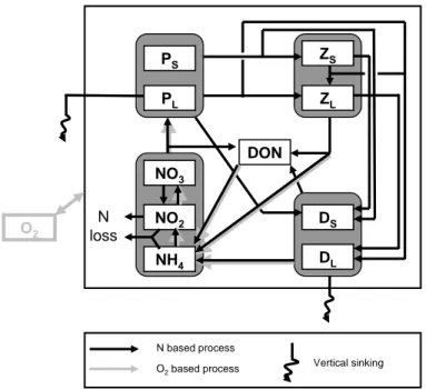
BioBUS (Fig. 2) is a nitrogen-based model derived from a N2P2Z2D2model (Kon ´e et

al., 2005), which has been successfully used to simulate the first trophic levels of the Benguela ecosystem. It takes into account the main planktonic communities and their specificities in the Benguela upwelling ecosystem. In this model, nitrate and ammo-nium represent the pool of dissolved inorganic N. Phytoplankton and zooplankton are

5

split into small (flagellates and ciliates, respectively) and large (diatoms and copepods, respectively) organisms. Detritus are also separated into small and large particulate compartments. We added a Dissolved Organic Nitrogen (DON) compartment. Indeed, DOM is an important reservoir of OM and plays an important role in supplying nitrogen or carbon from the coastal region to the open ocean (Huret et al., 2005). The

simu-10

lated DON is the semi-labile one as the refractory and labile pools of DON have too long (hundred of years) and too short (less than a day) turnover rates, respectively (Kirch-man et al., 1993; Carlson and Ducklow, 1995). The BioBUS model also includes nitrite to have a more detailed description of the microbial loop: ammonification/nitrification processes under oxic conditions, and denitrification/anammox processes under anoxic

15

conditions (Yakushev et al., 2007). These processes are oxygen-dependent, so an oxygen equation has been introduced in the BioBUS model. To complete this nitrogen-based model, N₂O was introduced using the Nevison et al. (2003) parameterization which allows to determine the N2O production in function of the oxygen amount

con-sumed by nitrification and the depth.

20

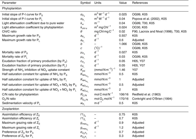
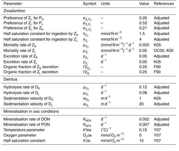
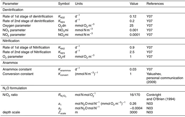
Interactions between the different compartments of the BioBUS model are summa-rized in Fig. 2. All state variables (Table 1) are expressed in mmol m−3. The formulation of the SMS terms for each of the biogeochemical tracers is given in Appendix A. Pa-rameter values are given in Table 2.

Due to different modifications and additions made from the original biogeochemical

25

model of Kon ´e et al. (2005), we had to adapt the BioBUS model, especially some of the parameter values within the range of parameter values found in the literature (Table 2). Indeed, parameters linked to the microbial loop (hydrolysis of detritus µD_S

(10)

BGD

8, 3537–3618, 2011

E. Gutknecht et al.

Title Page

Tables Figures

◭ ◮

Back Close

Full Screen / Esc

Discussion

P

a

per

|

Dis

cussion

P

a

per

|

Discussion

P

a

per

|

Discussio

n

P

a

per

|

matterKND4 from Yakushev et al. (2007) formulations, sinking velocity of large detritus

wD_L) were adjusted in order to better represent the distribution of nutrients and oxygen

from the coast to the open ocean. Also, as a more detailed representation of the nitrification was introduced in the BioBUS model as compared to Kon ´e et al. (2005), some of the parameter values associated with nutrients uptake by the phytoplankton

5

(half saturation constants KNO

3PS and KNH4PL) had to be adjusted in order to obtain

a better agreement for the chlorophyll-aconcentrations (Chl-a) between the simulated field and the data (see Sect. 4.3). We changed the grazing function with the introduction of the preference parameter for the zooplankton for different types of plankton (Dadou et al., 2001, 2004), as well as the associated maximum growth rates and half saturation

10

constants for ingestion. With these modifications, the general spatial distribution of the different types of plankton from the coast to the open ocean in the BUS is better simulated as compared to data (Kreiner and Ayon, 2008; Silio-Calzada et al., 2008).

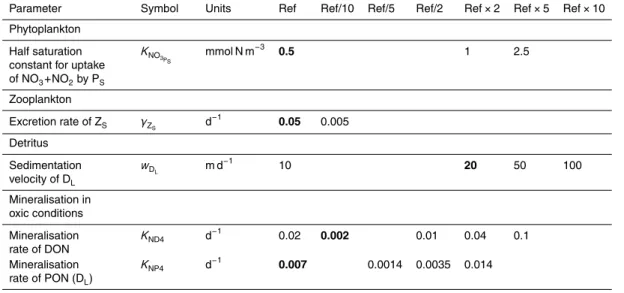
This first adjusted version of the model constitutes the reference run for the following analyses of the parameters. Then, the values of key parameters were adjusted

per-15

forming sensitivity analyses (Table 3). The methodology for these analyses consists in arbitrarily changing the value of these key parameters for the reference run. Parame-ters are modified one by one and their reference values are increased or decreased by a factor of 2 up to a factor of 10. For each analysis, the annual means of the simulated fields were compared with the annual climatologies of nitrate and oxygen

concentra-20

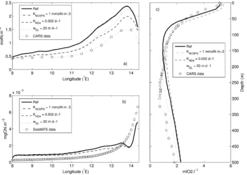
tions from the CSIRO Atlas of Regional Seas (CARS, 2006) and SeaWiFS Chl-a(see details on Sect. 3). The parameter value is chosen such as the difference between the simulated fields and the data for nitrates, oxygen and Chl-ais the smallest among the different tests we made. These adjustments are illustrated in Fig. 3 for the three parametersKND4,wD_L andKNO

3PS (Table 3) using different representative profiles.

25

The decrease by a factor of 10 of the DON mineralization parameter (KND4) induces

(11)

BGD

8, 3537–3618, 2011

E. Gutknecht et al.

Title Page

Tables Figures

◭ ◮

Back Close

Full Screen / Esc

Discussion

P

a

per

|

Dis

cussion

P

a

per

|

Discussion

P

a

per

|

Discussio

n

P

a

per

|

first 100 m of the vertical profile of oxygen concentrations (Fig. 3c). The doubling of the sedimentation sinking velocity parameter (wD_L) leads to a decrease of 15% of the 0–

100 m integrated nitrate concentrations, mainly outside the continental shelf (Fig. 3a), and a decrease of 10% of the oxygen concentrations below 200 m on the continental shelf, both in better agreement with data (Fig. 3c). The very small e_ffect of doubling the

5

phytoplankton nutrient half-saturation coefficient (KNO

3PS) on surface Chl-a (Fig. 3b),

nitrate and oxygen concentrations justifies our choice to keep this parameter at a low value (KNO

3PS =0.5 mmol N m −3

as for the reference run). Using these sensitivity anal-yses, we also decreased the small zooplankton specific excretion rateγZ_S by a factor of

2 in order to add an additional decreasing effect on the ammonium and nitrite

concen-10

trations, already existing with thewD_L andKND4adjustments (data not shown). Finally,

the maximum growth rate of the large phytoplankton (diatoms) had to be reduced from 0.8356 d−1 (Kon ´e et al., 2005) to 0.6 d−1 (Fasham et al., 1990; Oschlies and Garcon, 1999; Huret et al., 2005) to obtain a better agreement between the simulated primary production and the BENEFIT data from Barlow et al. (2009) as well as the data from

15

the Atlantic Meridional Transect (AMT) in May 1998 (AMT 6 cruise), especially in the coastal area (see Sect. 4.3).

2.3 The Namibian configuration

The ROMS Namibian configuration (Fig. 1) is built on a Mercator grid, spanning 5◦E to 17◦E and 19◦S to 28.5◦S with a horizontal resolution of 1/12◦(ranging from 8.15 km in

20

the south to 8.8 km in the north). The grid has 32 sigma-levels stretched so that near-surface resolution increases. In the coastal area, with a minimum depth of 75 m, the thickness of the first (at the bottom of the ocean) and last (near the ocean-atmosphere interface) levels is 11.4 m and 0.4 m, respectively. In the open-ocean area, with a maximum depth of 5000 m, the thickness of the first and last levels is 853.5 m and 5 m,

25

(12)

BGD

8, 3537–3618, 2011

E. Gutknecht et al.

Title Page

Tables Figures

◭ ◮

Back Close

Full Screen / Esc

Discussion

P

a

per

|

Dis

cussion

P

a

per

|

Discussion

P

a

per

|

Discussio

n

P

a

per

|

The ROMSTOOLS package (Penven et al., 2008, http://roms.mpl.ird.fr) has been used to build the model grid, atmospheric forcing, initial and boundary conditions.

The Namibian configuration used in this study is a small domain which is a sub-domain of the SAfE HR climatological configuration (Veitch et al., 2009) (Fig. 1). For temperature, salinity, free surface and the velocity (zonal and meridional components),

5

the initial conditions come from 1 January of the 10th year of SAfE HR (Veitch et al., 2009); the open boundary conditions are also provided by the 10th year of this simula-tion for which variables have been averaged every 5 days.

A 1/2◦ resolution QuikSCAT (Liu et al., 1998) monthly climatological wind stress (courtesy of N. Grima, LPO, Brest, France) based on data spanning from 2000 to

10

2007 is used to force the model at the surface. Surface heat and salt fluxes are pro-vided by 1/2◦resolution COADS-derived monthly climatology (Da Silva et al., 1994). An air-sea feedback parameterization term, using the 9-km Pathfinder climatological Sea Surface Temperature (SST) (Casey and Cornillon, 1999), is added to the surface heat flux to avoid model SST drift (Barnier et al., 1995; Marchesiello et al., 2003). A similar

15

correction scheme is used for Sea Surface Salinity (SSS) because of the paucity of evaporation-precipitation forcing fields as in Veitch et al. (2009).

For the biogeochemistry, the initial and the open boundary conditions for NO3 and

O2concentrations are provided by the month of January and the monthly climatology of

the CARS database (2006), respectively. Other biogeochemical tracers are initialized

20

using a constant profile (see Table 1); the same constant profiles are used for the open boundary conditions.

The simulation is run for a total of 12 yr. A physical spin-up is performed over 7 yr, as the model needs a few years to reach a stable annual cycle, then the coupled physical/biogeochemical model is run for 5 yr. The last year of simulation (year 12) will

25

(13)

BGD

8, 3537–3618, 2011

E. Gutknecht et al.

Title Page

Tables Figures

◭ ◮

Back Close

Full Screen / Esc

Discussion

P

a

per

|

Dis

cussion

P

a

per

|

Discussion

P

a

per

|

Discussio

n

P

a

per

|

3 Satellite and in-situ data used

In the studied area, simulated fields are compared with different types of available data sets.

Chl-afrom the monthly climatology SeaWiFS products of level 3-binned data (9 km, version 4, O’Reilly et al., 2000), from 1997 to 2009, processed by the NASA Goddard

5

Space Flight Center and distributed by the DAAC (Distributed Active Archive Center) (McClain et al., 1998), are used for comparison with surface simulated Chl-a. Simu-lated Chl-ais the sum of flagellate and diatom concentrations expressed in N units and converted into Chl-a(mg Chl m−3) using a variable ratio described in Appendix A.

Di_fferent sections and stations are used for the model/data comparison. Their

po-10

sitions are shown in Fig. 4. Temperature, salinity, oxygen, nutrients, Chl-a, primary production, and mesozooplankton data were collected in May 1998 during the AMT 6 cruise (Aiken, 1998; Aiken and Bale, 2000; Aiken et al., 2000). Samples were collected during expeditions M57/2 of R/VMeteor February 2003 (Zabel et al., 2003; Kuypers et al., 2005) and AHAB1 of R/VAlexander von Humboldt in January 2004 (Lavik et

15

al., 2009), and allowed to estimate temperature, salinity, oxygen and nutrients in the Namibian upwelling system. In October 2006, the Danish Galathea expedition crossed the BUS. Measurements of temperature, salinity, oxygen, nutrients, and Chl-a were collected (courtesy of L. L. Søerensen, National Environmental Research Institute, Denmark) at different stations and along a vertical section (triaxus system

undulat-20

ing vertically and laterally off the stern of the ship). A mooring located on the outer shelf at 23◦S in Walvis Bay between 1994 and 2004 (Monteiro and van der Plas, 2006) allowed to obtain a time series of temperature, salinity and oxygen. Measurements of copepod abundance integrated over 200 m, from the coast (14.5◦E) to 70 nautical miles (13.23◦E) at 23◦S in Walvis Bay, were collected between 2000 and 2007 (Kreiner and

25

(14)

BGD

8, 3537–3618, 2011

E. Gutknecht et al.

Title Page

Tables Figures

◭ ◮

Back Close

Full Screen / Esc

Discussion

P

a

per

|

Dis

cussion

P

a

per

|

Discussion

P

a

per

|

Discussio

n

P

a

per

|

temperature and salinity fields (CARS, 2009), and oxygen and nitrate concentrations (CARS, 2006). The World Ocean Atlas (WOA) 2001 includes a global climatology of Chl-a(Conkright et al., 2002). The AMT 17 cruise in November 2005 estimated DON concentrations in the Southern Benguela. For the first time in the Namibian upwelling system, N2O samples were collected at 9 stations offWalvis Bay at around 23

◦

S

dur-5

ing the FRS Africana cruise, in December 2009 within the framework of the GENUS project (Geochemistry and Ecology of the Namibian Upwelling System). The collected samples were poisoned with mercuric chloride on board and measurements were done after the cruise at IFM-GEOMAR, Germany by using the static equilibration method ac-cording to Walter et al. (2006).

10

All data enumerated above will be compared to simulated ones for the same ge-ographical positions (except for DON because there are no available measurements in the Namibian upwelling system) and the same climatological months. Simulated oxygen concentrations are converted in ml O₂l−1for comparison with in-situ data.

4 Model/data comparison

15

To compare simulated fields m and data d (in-situ and satellite data considered as the reference), different statistical metrics are selected: the mean (M), the bias (Mm−

M_d), the Root Mean Square (RMS), the standard deviation (σ), and the correlation coefficient (R). The centered pattern RMS difference (E′) is formulated as E′2=σm2+

σ_d2−2σmσdR. The centered pattern RMS difference and the two standard deviations

20

are normalized by the standard deviation of the dataσ_d. Then, the normalized standard deviation of the simulated field isσ∗=σ_m∗ =σ_m/σ_d, the normalized standard deviation of the data isσ_d∗ =1, and the normalized centered pattern RMS di_fference becomesE′∗=

E′/σ_d =pσ∗2₊₁₋_2σ∗_{R. The statistical information (E}′∗_, _σ∗_, _{R), referred as “pattern}

statistics”, is summarized in Taylor’s diagrams (Taylor, 2001).

(15)

BGD

8, 3537–3618, 2011

E. Gutknecht et al.

Title Page

Tables Figures

◭ ◮

Back Close

Full Screen / Esc

Discussion

P

a

per

|

Dis

cussion

P

a

per

|

Discussion

P

a

per

|

Discussio

n

P

a

per

|

4.1 Temperature, salinity, and density

For the temperature field (Fig. 5a), the correlation coefficient between simulated fields and data is above 0.93 for all stations and sections except for the Galathea data (sur-face and station data;R=0.86). The normalized standard deviation for temperature is between 0.9 and 1.2 for all comparisons; except for the Galathea data (σ∗ is between

5

1.3 and 1.4). The normalized centered pattern RMS difference is less than 0.4, ex-cept for the Galathea data (E′∗=0.5 for triaxus data, or a RMS difference of 1.41◦C; E′∗=0.67 for surface and station data, or a RMS difference of 1.43◦C). The differences between model and data averages (called bias) for temperature vary from 0.25 to 1.2◦C along the METEOR 57/2 sections, from−0.33 to 0.52◦C for the AHAB1 sections, from

10

0.6 to 1◦C for the Galathea data, and from 0.2 to 1.2◦C for the AMT 6 data.

For the salinity field (Fig. 5b), the correlation coefficient between simulated fields and data is above 0.74 for all stations and sections, except for Galathea data (station and surface data;R=0.62). The normalized standard deviation is between 0.55 and 1.2 for all data, except for four Galathea triaxus (σ∗=1.55). The normalized centered

15

pattern RMS difference is less than 0.7, except for the Galathea surface and station data (E′∗=0.95, or a RMS difference of 0.15). Biases for salinity vary from −0.05 to 0.08 along the METEOR 57/2 sections, from−0.2 to−0.001 for the AHAB1 sections, from 0.04 to 0.1 for Galathea data, and from−0.22 to−0.009 for the AMT 6 data.

The same comparison is made for the density field. Density is computed from

tem-20

perature and salinity in-situ data, using the same Jackett and McDougall (1995) re-lationship that one used in ROMS. The correlation coefficient between simulated and in-situ density is above 0.9 for all stations and sections (Fig. 5c). The normalized stan-dard deviation is between 0.85 and 1.4 for all comparisons; and the normalized cen-tered pattern RMS difference is less than 0.52 (the range of RMS difference is between

25

0.13 and 0.29 kg m−3). Bias for density varies from−0.26 to−0.06 kg m−3.

(16)

BGD

8, 3537–3618, 2011

E. Gutknecht et al.

Title Page

Tables Figures

◭ ◮

Back Close

Full Screen / Esc

Discussion

P

a

per

|

Dis

cussion

P

a

per

|

Discussion

P

a

per

|

Discussio

n

P

a

per

|

observed in the surface layer (0–100 m) over the continental shelf. No clear latitudinal trend can be highlighted. The results of these statistics point out an important interan-nual variability for the in-situ data which is not represented by our simulation. Indeed, the monthly climatological fields (winds, heat and fresh water fluxes) used to force the model are repeated each year, with a linear interpolation between each month, so the

5

forcing fields are smoothed in time.

To complete the model/data comparison, the same statistics for the annual mean and the seasonal cycle are computed between the simulated fields and the climatology from CARS database (2009). The comparison between seasonal fields is performed between the surface and 600-m depth. Below this depth, statistics do not show

sea-10

sonal variation (not shown). The annual fields are also compared in the top 600 m as well as over the whole water column. The statistics were added in the Taylor’s diagrams for temperature, salinity, and density (see the last six points in Fig. 5a, b, and c). The correlation coe_fficient between simulated fields and CARS database (2009) is above 0.98 for temperature, and above 0.96 for salinity and density. The normalized standard

15

deviation is between 0.9 and 1 for temperature, between 0.8 and 1 for salinity, and be-tween 0.85 and 1 for density. The normalized centered pattern RMS difference is less than 0.21 (or a RMS difference of 0.9◦C) for temperature, 0.3 (or a RMS difference of 0.1) for salinity, and 0.3 (or a RMS difference of 0.17 kg m−3) for density. Biases vary between 0.09 and 0.29◦C,−0.05 and−0.01 for salinity,−0.07 and−0.02 kg m−3.

20

To illustrate the above Taylor’s diagrams, two types of model/data distributions in space and time are presented along a section (23◦S; Figs. 6 and 7) and at a moor-ing point (23◦S–14◦E; Fig. 11). Monthly averaged simulated fields and in-situ mea-surements of temperature, salinity and density along the 23◦S METEOR 57/2 section (east-west direction in February 2003) are displayed in Fig. 6. On the shelf,

tempera-25

(17)

BGD

8, 3537–3618, 2011

E. Gutknecht et al.

Title Page

Tables Figures

◭ ◮

Back Close

Full Screen / Esc

Discussion

P

a

per

|

Dis

cussion

P

a

per

|

Discussion

P

a

per

|

Discussio

n

P

a

per

|

as for the 23◦S METEOR 57/2 section. Figure 7 presents the annual mean of tem-perature, salinity, and density at 23◦S as compared with the annual climatology from CARS database (2009). Simulated fields are in agreement with the data: the vertical profile of temperature, salinity, and density are correctly simulated, although simulated salinity is weaker than measured salinity in the surface one, especially near the coast.

5

This bias seems to come from the SSS corrections used in the model configuration. Indeed, the SSS values from the COADS climatology used for the correction scheme in the salt fluxes (Sect. 2.3) are lower than in-situ data and CARS climatology (2009) at 23◦S (not shown).

The temporal evolution of the vertical profiles of simulated temperature and salinity

10

at 23◦S–14◦E (Fig. 11) is compared to the time series at this Walvis Bay mooring (Fig. 4 for location) (see figure 5-3 from Monteiro and van der Plas, 2006). The same vertical structure in time is observed between the simulated fields and in-situ data. Temperature around 17–18◦C is observed each summer in the surface layer, isotherms 13◦C and 10◦C are situated around 100 and 300-m depth, respectively. Isohaline 35 is

15

located at a mean depth of 200 m, with salinity up to 35.2 between the surface and 100-m depth, and fresher water intrusions around 34.8 occur each year at 300-100-m depth.

These statistics show that the model is able to simulate the annual mean and sea-sonal cycle for temperature, salinity, and density over the Namibian upwelling system despite a lower standard deviation.

20

4.2 Oxygen, nitrate, nitrite, and ammonium

The model correctly simulates the OMZ located along the continental slope (Figs. 8a and 9a), with more depleted waters in the northern part of the domain (between 19◦S and 24–25◦S) where the South Atlantic Central Waters (SACW; Mohrholz et al., 2008) are present. The di_fferences between model and data averages for oxygen

concentra-25

tions are always positive from 0.14 to 0.66 ml O2l −1

along the METEOR 57/2 sections, from 0.03 to 1.6 ml O2l

−1

for the AHAB1 sections, from 0.18 to 0.8 ml O2l −1

for the Galathea data, and 0.68 ml O2l

−1

(18)

BGD

8, 3537–3618, 2011

E. Gutknecht et al.

Title Page

Tables Figures

◭ ◮

Back Close

Full Screen / Esc

Discussion

P

a

per

|

Dis

cussion

P

a

per

|

Discussion

P

a

per

|

Discussio

n

P

a

per

|

to the overestimation of oxygen concentrations on the continental shelf for water-depth above 200 m. The correlation coe_fficient between simulated and in-situ oxygen concen-trations varies between 0.55 and 0.97 for all data (Fig. 10a). The normalized standard deviation is lower than 1 for all comparisons. Standard deviation or variations of the simulated oxygen concentrations are lower than for in-situ measurements, mainly

as-5

sociated with interannual variability in the BUS. The normalized centered pattern RMS difference is less than 0.85 for all data. The RMS difference is between 0.34 and 2.35 ml O₂l−1.

To complete the statistics, the seasonal cycle and annual mean of simulated oxygen concentrations are compared with CARS database (2006). For all comparisons with

10

CARS, the correlation coe_fficient is between 0.87 and 0.93, and the normalized stan-dard deviation is between 0.85 and 0.95 (Fig. 10a). Biases vary between −0.1 and 0.09 ml O2l

−1

. Compared to the CARS database (2006) (Fig. 9a), the vertical struc-ture of oxygen concentrations is well simulated, except on the continental shelf where the OMZ occurs. In our simulation, the OMZ is located on the slope as for the CARS

15

database (2006) but does not extend enough on the continental shelf. The same ob-servation can be made when the temporal evolution of the vertical profiles of oxygen concentrations at 23◦S–14◦E (Fig. 11) is compared with the time series of oxygen con-centrations at the Walvis Bay mooring (see figure 5-3 from Monteiro and van der Plas, 2006). The oxygen seasonal cycle is correctly represented. Concentrations between 6

20

and 7 ml O2l −1

are well simulated close to the surface, while they are frequently lower than 1 ml O2l

−1

at depth. However, concentrations below 0.5 ml O2l −1

are frequently recorded at this mooring while they remain higher than 0.5 ml O2l

−1

in our simulation. So, the model correctly simulates the vertical distribution of oxygen but in-situ concen-trations are more depleted at depth than the simulated ones. We will comment this

25

difference in the following paragraph.

(19)

BGD

8, 3537–3618, 2011

E. Gutknecht et al.

Title Page

Tables Figures

◭ ◮

Back Close

Full Screen / Esc

Discussion

P

a

per

|

Dis

cussion

P

a

per

|

Discussion

P

a

per

|

Discussio

n

P

a

per

|

is located at depth between 200 and 1500 m (with variations depending on latitude and related to the upwelling cells along the coast). The di_fferences between model and data averages for nitrate concentrations are from−2.7 to−1.66 mmol N m−3along the METEOR 57/2 sections, from −5 to 1.66 mmol N m−3 for the AHAB1 sections, −0.02 mmol N m−3for the Galathea stations, and−7.9 mmol N m−3for the AMT 6 data.

5

Hence, simulated nitrate concentrations are in general underestimated. The corre-lation coefficient between simulated and in-situ nitrate concentrations is between 0.8 and 0.94 for Galathea, AMT 6, and METEOR 57/2 data, with normalized standard de-viations between 0.59 and 1.21, and normalized centered RMS differences less than 0.65 (RMS difference: 6.1 mmol N m−3) (Fig. 10b). The statistics are worse for AHAB1

10

data in January 2004, but this period was particular because an important sulphidic event was recorded in the continental shelf waters off Namibia (Lavik et al., 2009) during this cruise. North of 27◦S, oxygen-depleted waters (O2<0.1 ml O2l

−1

) were recorded below 60-m depth. In oxygen-depleted environments, the best electron ac-ceptor for anoxic remineralization (denitrification) is nitrate. When oxygen and nitrate

15

are depleted, sulfate reduction produces toxic hydrogen sulfide, as measured during the AHAB1 cruise. This extreme event generally occurs on or close to the sediments on the continental shelf, and our biogeochemical model does not include the sediment processes. In order to improve our model and simulate very low oxygen concentrations on the continental shelf, a sediment module has to be added to BioBUS.

20

As for the other variables, the seasonal cycle and annual mean of simulated nitrate concentrations are now compared with CARS database (2006). The correlation co-efficient is higher than 0.94, and the normalized standard deviation is between 0.9 and 1.05. The normalized centered pattern RMS difference is less than 0.35 (or a RMS difference of 3.4 mmol N m−3) for all comparisons with CARS climatology (2006)

25

(20)

BGD

8, 3537–3618, 2011

E. Gutknecht et al.

Title Page

Tables Figures

◭ ◮

Back Close

Full Screen / Esc

Discussion

P

a

per

|

Dis

cussion

P

a

per

|

Discussion

P

a

per

|

Discussio

n

P

a

per

|

The other nutrients, i.e. nitrite and ammonium, present very low values in the sim-ulation with maximum value of 0.14 and 0.4 mmol N m−3, respectively, located in the surface layer above the continental shelf. These two nutrients are fastly transformed in nitrate by the nitrification processes. For the AHAB1 cruise, concentrations up to 1 and 4 mmol N m−3 were measured for nitrite and ammonium concentrations, respectively.

5

These high values were principally observed on the continental shelf. The Galathea cruise measured nitrite concentrations up to 0.67 mmol N m−3in the studied area. Dur-ing this cruise, ammonium concentrations below the detection level of 0.3 mmol N m−3 were found all over the region, and the model is able to reproduce this pattern. During AMT 6 cruise, nitrite was measured at four stations in our studied area.

Concen-10

trations vary from 0.01 to 0.43 mmol N m−3. Only two measurements of ammonium concentrations are available for this latter cruise: 0.62 mmol N m−3at 161-m depth and 3.13 mmol N m−3 at 22-m depth (located at the same station 26.7◦S–14.25◦E). We do not have enough in-situ measurements of nitrite and ammonium concentrations to con-clude, but simulated fields seem to have the same order of magnitude as in-situ data,

15

maybe at the lower limit of the measured concentrations.

The model is able to simulate the annual mean and seasonal cycle for nitrate, and oxygen concentrations. Vertical gradients of simulated oxygen and nitrate concentra-tions as well as horizontal distribuconcentra-tions give satisfying results, except oxygen concen-trations near the sediment-water interface over the continental shelf. Simulated nitrite

20

and ammonium concentrations are within the range of available in-situ data.

4.3 Chlorophyll-aand total primary production

Simulated surface Chl-a are around 0.25 mg Chl m−3 offshore, being higher than those derived from SeaWiFS sensor (0.2 mg Chl m−3; Fig. 12). Chl-a increase up to 10 mg Chl m−3 at the coast (Fig. 12) in the model, in agreement with satellite data.

25

(21)

BGD

8, 3537–3618, 2011

E. Gutknecht et al.

Title Page

Tables Figures

◭ ◮

Back Close

Full Screen / Esc

Discussion

P

a

per

|

Dis

cussion

P

a

per

|

Discussion

P

a

per

|

Discussio

n

P

a

per

|

part of the domain, while it is more diffusive in the northern part. The simulated Chl-a is now compared with the annual WOA climatology (2001; Conkright et al., 2002) along three vertical sections (21.5◦S, 23.5◦S, and 25.5◦S; Fig. 13) in order to evaluate the performance of the modeling experiment in reproducing the vertical distribution. At 100-m depth, simulated and in-situ Chl-a are lower than 0.2 mg Chl m−3. Maximum

5

Chl-a are observed between the surface and 40–50 m depth in both data sets. At 21.5◦S and 23.5◦S, simulated Chl-a are lower than in-situ data in the surface layer; high simulated Chl-a are confined close to the coast. As the resolution of the WOA climatology (2001; Conkright et al., 2002) is too coarse, we used in-situ data from the Galathea and AMT 6 cruises to evaluate the simulated distribution of Chl-a.

10

Concerning the Galathea cruise (October 2006), three values of Chl-ain Walvis Bay (St. 6.7, in the middle of the domain) are available: one estimation at 10-m depth (1.16 mg Chl m−3), another at 75-m depth (0.14 mg Chl m−3), and a value integrated over the first 71-m depth (57.8 mg Chl m−2). At the same location and same depths, simulated Chl-aare equal to 1.5 mg Chl m−3, 0.2 mg Chl m−3, and 69.5 mg Chl m−2,

re-15

spectively, so in close agreement with measurements. During the AMT 6 cruise in May 1998, vertical profiles of Chl-a were estimated by four di_fferent sources (E. Fernan-dez, P. Holligan, R. Barlow, and the British Oceanographic Data Center; Barlow et al., 2002, 2004) at three stations situated in the middle of our domain (St. 14, 15, and 16; Fig. 14). Vertical profiles of simulated Chl-a are within the di_fferent estimations. The

20

sub-surface maximum (between 10 and 40 m) observed at St. 15 is well represented by the model with Chl-a reaching 1.4 mg Chl m−3. At 62-m depth (St. 15), observed Chl-aare between 0.43 and 0.81 mg Chl m−3, and simulated concentration is equal to 0.4 mg Chl m−3. The vertical structures as well as the range of the simulated Chl-aare quite in agreement with the few available data.

25

(22)

BGD

8, 3537–3618, 2011

E. Gutknecht et al.

Title Page

Tables Figures

◭ ◮

Back Close

Full Screen / Esc

Discussion

P

a

per

|

Dis

cussion

P

a

per

|

Discussion

P

a

per

|

Discussio

n

P

a

per

|

coast. Based on satellite observations, Silio-Calzada et al. (2008) estimated that 39% of the total Chl-aare represented by nanophytoplankton on annual mean and over the same domain. This plankton community contributes to 50% in the open ocean and less than 20% along the coast. The model is in agreement with those satellite estimations. Silio-Calzada et al. (2008) also assessed that 24% of the total Chl-a are due to

pico-5

phytoplankton in the Namibian ecosystem, with an increasing contribution as we move offthe coast. In the eastern part of the domain, picophytoplankton contributes to 40% of total Chl-a. This phytoplankton population is not taken into account in BioBUS, so its contribution is partitioned between diatoms and flagellates. However, results from Silio-Calzada et al. (2008) should be taken with caution since their algorithm has not

10

been validated with in-situ data in the BUS.

Simulated total primary production is now compared with the BENEFIT data from Barlow et al. (2009). During summer (February–March), simulated total primary pro-duction integrated over the euphotic zone reaches 6 g C m−2d−1 near the coast. In winter (June–July), it reaches 3 g C m−2d−1 near the coast. In our modeling

experi-15

ment, the Namibian system appears to be twice more productive in summer than in winter. Along the Namibian coast, Barlow et al. (2009) estimated total primary produc-tion between 0.39 and 8.83 g C m−2d−1 during February–March 2002, and between 0.14 and 2.26 g C m−2d−1during June–July 1999. Spatial variations are important. For example, between St. FM18, FM19 and FM20 (located close to the coast; see Fig. 1

20

in Barlow et al., 2009), primary production varies from 1.5 to 6.7 g C m−2d−1 during summer 2002. At St. FM 24 located more offshore, primary production was measured at 2 g C m−2d−1, the model giving the same value for this location. Simulated total primary productions are within the range of values estimated by Barlow et al. (2009) for summer time, but are much higher than those measured during winter 1999. But

25

(23)

BGD

8, 3537–3618, 2011

E. Gutknecht et al.

Title Page

Tables Figures

◭ ◮

Back Close

Full Screen / Esc

Discussion

P

a

per

|

Dis

cussion

P

a

per

|

Discussion

P

a

per

|

Discussio

n

P

a

per

|

remain some months (Shannon et al., 1986). Therefore the upwelling of nutrient-rich waters decreases and primary production is lower than usual for some time. Siegfried et al. (1990) reported that during previous Benguela Ni ˜no events, primary productivity has been reduced by more than two thirds.

During the AMT 6 cruise in May 1998 (Aiken, 1998; Aiken and Bale, 2000; Aiken

5

et al., 2000), total primary production was estimated at three stations within our stud-ied area. Simulated and in-situ total primary productions were integrated over the euphotic zone as Barlow et al. (2009) (simulated euphotic zone is between 20 and 37-m depth at the three studied stations). At St. 12, the simulated primary produc-tion is higher (3.9 g C m−2d−1) than in-situ primary production (1.6 g C m−2d−1). At

10

St. 15 (St. 18), simulated and in-situ values are similar, with 3.3 (3.55 g C m−2d−1) and 3.26 g C m−2d−1(3.32 g C m−2d−1), respectively. At the three stations, the surface pri-mary production is higher than in-situ data, the difference decreases until∼25-m depth. Below this limit, simulated and in-situ estimations of primary production are similar, and they are close to 0 at 50-m depth.

15

Spatio-temporal variability of primary production is pretty well captured in our mod-eling experiment even if direct comparisons are di_fficult to analyze in such a dynamic environment.

4.4 Zooplankton and DON

The temporal evolution of simulated copepod (mesozooplankton: large zooplankton

20

or Z_L in the model) abundance (number of individuals per m2: no m−2) at 23◦S is compared with in-situ data from Kreiner and Ayon (2008) (Fig. 15). Integrated over 200-m depth, in-situ data between 2000 and 2007 present an important interannual variability. However, the maximum abundance is usually observed during the first part of the year (summer–early fall, with 1.105 to 7.105 no m−2) and is located between

25

(24)

BGD

8, 3537–3618, 2011

E. Gutknecht et al.

Title Page

Tables Figures

◭ ◮

Back Close

Full Screen / Esc

Discussion

P

a

per

|

Dis

cussion

P

a

per

|

Discussion

P

a

per

|

Discussio

n

P

a

per

|

mass for Calanoides Carinatus (juvenile, and adult stages) as estimated by Huggett et al. (2009), a major copepod species in the Namibian system. Biomass was converted in terms of carbon by assuming that 40% of the dry weight was carbon (Peterson et al., 1990). The C/N ratio of 5.36 used for mesozooplankton biomass comes from AMT 6 (Aiken, 1998; Aiken and Bale, 2000; Aiken et al., 2000) estimations in this area.

5

As shown in Fig. 15, the model simulates a maximum of copepod abundance during summer–early fall, situated at the same distance from the coast as in-situ data. Each year of the climatological simulation, the simulated copepod abundance varies between 1.105and 5.105no m−2.

During AMT 6 cruise, zooplankton was estimated at three stations (St. 15, 12, and

10

7; see Fig. 4). Data from di_fferent size classes (200–500 µm, 500–1000 µm, 1000– 2000 µm, >2000 µm) were integrated over 200-m depth except for St. 12 where inte-gration were performed over 100-m depth. To compare with our simulation, we only take into account the fraction comprised between 200 and 2000 µm, usually consid-ered as mesozooplankton (copepods in the model). During the cruise,

mesozooplank-15

ton was estimated at a value of 796.5 mg N m−2 at St. 15, 2204.6 mg N m−2 at St. 12, and 357.5 mg N m−2 at St. 7. For the same climatological month and the same loca-tions, the simulated concentrations are around 750, 200, and 150 mg N m−2. At St. 15, simulated and in-situ concentrations have similar values. At St. 12 and 7, simulated concentrations are much lower than in-situ data maybe due to in-situ sampling

col-20

lected in an enriched structure (filament, eddy). Indeed, if we do not take the value at exactly the same location, but in a physical structure, simulated mesozooplankton con-centrations can reach 1100 mg N m−2. This range of value comes closer to the in-situ observations.

Simulated semi-labile DON is compared with data from the AMT 17 cruise conducted

25

(25)

BGD

8, 3537–3618, 2011

E. Gutknecht et al.

Title Page

Tables Figures

◭ ◮

Back Close

Full Screen / Esc

Discussion

P

a

per

|

Dis

cussion

P

a

per

|

Discussion

P

a

per

|

Discussio

n

P

a

per

|

refractory DON, and we removed this refractory part (assumed constant with depth) of the vertical profile of DON. Simulated vertical profiles of semi-labile DON concen-trations were taken offshore, one in a physical structure (a filament) and another one outside of this structure (Fig. 16). Simulated and in-situ profiles are not directly com-parable but in-situ concentrations give an indication on the profiles we can expect to

5

find offshore of our domain. Simulated DON concentrations are within the range of in-situ concentrations (Fig. 16). The three eastern stations of AMT 17 seem to be out offa physical structure, while the station at 33.9◦S–10.3◦E could be in a filament or an eddy.

4.5 N₂O distribution

10

In Fig. 17, the vertical sections of temperature, salinity, and oxygen concentrations off

Walvis Bay derived from modeled fields show the signature of an upwelling event due to intense alongshore winds. A similar situation was observed during the FRS Africana cruise in December 2009 as strong winds lead to upwelling of oxygen-depleted subsur-face waters intersecting the sursubsur-face within a narrow strip (15–20 nm) along the coast

15

around Walvis Bay (Mohrholz et al., 2009 in Cruise Report from Ekau and Verheye, 2009).

In-situ N₂O concentrations reached up to approximately 40 nmol N₂O l−1 in oxygen-depleted waters in the water column onto the shelf, and at the shelf break near the water-sediment interface and tend to decrease with increasing O2 concentrations

20

(Fig. 17c and d). Simulated N₂O concentrations have similar values as compared to data for waters with O2concentrations above 2.6 ml O2l

−1

(Fig. 17c and d). For lower O2concentrations, simulated N2O concentrations are underestimated as compared to

measured ones, with a maximum of 20 nmol N₂O l−1 over the shelf and shelf-break (Fig. 17d). The parameterization used in BioBUS (see Appendix A) from Nevison et

25

al. (2003) only takes into account N2O formation associated with oxygen consumption

(26)

BGD

8, 3537–3618, 2011

E. Gutknecht et al.

Title Page

Tables Figures

◭ ◮

Back Close

Full Screen / Esc

Discussion

P

a

per

|

Dis

cussion

P

a

per

|

Discussion

P

a

per

|

Discussio

n

P

a

per

|

will probably improve results for the N₂O distribution in the whole ocean including OMZ. This parameterization will be implemented and tested in BioBUS in a future work.

5 Nitrogen budget in the Walvis Bay area: nitrogen transfers and air-sea

N₂O fluxes

The nitrogen (N) budget is performed around Walvis Bay between 22◦S and 24◦S and

5

from the coast to 12.5◦E. Walvis Bay is chosen because the OMZ is well developed in this area (Mohrholz et al., 2008; Monteiro et al., 2008). To understand the hori-zontal and vertical transfers of N from the coast to the open ocean, the studied area is divided in two sub-domains: the coastal domain which represents the continental shelf from the coast to the 200-m isobath and the continental slope domain which is

10

considered to be situated between the 200-m isobath and the 2500-m isobath. These two sub-domains are divided in three layers: the surface layer down to 100-m depth (maximum depth of the mixed layer in the ocean in austral winter); the intermediate layer between 100 and 600-m depth where the OMZ is located; and the oxic bottom layer between 600 and 5000-m depth. Note that the volume of each sub-domain is

15

different, and then integrated fluxes (in 1010mol N yr−1) presented in Figs. 18 and 19 cannot be directly compared from a sub-domain to the other. In the following, the area called “entire Walvis Bay domain” corresponds to 22◦S–24◦S, from the coast to 10◦E. For comparisons with other studies, we took a C/N Redfield ratio (106/16; Redfield et al., 1963) for the conversion of fluxes from nitrogen to carbon.

20

5.1 Physical forcing and associated export

As shown in Fig. 18, two main areas of upwelling are found. Nitrate-rich SACW waters upwell over the slope (17.7×1010mol N yr−1) at 100-m depth: 8×1010mol N yr−1 are upwelled at 50-m depth, 5.9×1010mol N yr−1advected onshore between 50 and 100 m and, and 8.6×1010mol N yr−1advected offshore between 50 and 100-m depth. Above

(27)

BGD

8, 3537–3618, 2011

E. Gutknecht et al.

Title Page

Tables Figures

◭ ◮

Back Close

Full Screen / Esc

Discussion

P

a

per

|

Dis

cussion

P

a

per

|

Discussion

P

a

per

|

Discussio

n

P

a

per

|

the continental shelf off Walvis Bay area, 6.5×1010mol N yr−1 upwell at 50-m depth. Then, the Ekman transport advects nitrate enriched waters offshore between 0 and 50-m depth: 9.2×1010mol N yr−1are advected between the continental shelf and the slope sub-domains, 16.8×1010mol N yr−1between the slope sub-domain and the open ocean. The alongshore Benguela current also advects nutrient-rich waters from the

5

L ¨uderitz upwelling cell to the Northern Benguela system. As expected, the meridional advection due to the coastal Benguela current between 0 and 100-m depth has the most important contribution on the continental shelf (9.6+2.7= +12.3×1010mol N yr−1) and decreases with distance to the coast (5.3+3.5= +8.8×1010mol N yr−1 on the slope). In the coastal domain, the meridional advection of the Benguela current

10

represents the main contribution for sustaining primary production (between 0 and 100-m depth). From the surface to 100-m depth, zonal advection exports nitrates (9.2–5.9=3.3×1010mol N yr−1) offshore from the coast to the slope sub-domain, 25.4 (=16.8+8.6) 1010mol N yr−1from the slope sub-domain to the open ocean (Fig. 18).

Between 100 and 600-m depth, inshore zonal current advects nitrate enriched

wa-15

ters with an inshore decreasing contribution. At this depth range over the slope, the poleward undercurrent below the Benguela current advects nitrate enriched waters southward and represents a sink for the studied area with a maximum value over the continental slope.

5.2 Primary and secondary productions

20

Diatom biomass contributes to 99.2% of total primary production along the continental shelf, and 92% along the continental slope. Total primary production is largely sus-tained by nitrates: nitrates contribute to 87.7% of total primary production along the continental shelf and 80.8% along the slope. Primary production due to ammonium is not negligible and explains 11.9% of total primary production on the shelf and 17.9% on

25