Delineating SPECT Lung Contours using 3D Snakes

Abstract—To develop an automated 3D SPECT lung

delineation method by coupling adaptive dual exponential thresholding with 3D active contours. Datasets of Monte Carlo simulations and real subject scans with normal/low maximum and/or total count values were used as the basis of this study. After removing background noise using dual exponential thresholding, planar Gaussian filter and Sobel kernels are then used for edge enhancement, followed by final contour delineation via 3D active contours. Both quantitative validation via statistical measures and qualitative verification by experienced physicians were implemented to evaluate the method. We continue to achieve an overall congruency of 90% for both simulations and subject scans that are either normal or considered to be low in maximum and/or total count values. However, a slight 3-5% drop in congruency was observed, suggesting slight over-delineation by the proposed method. Although the results are still clinically very satisfactory, this study sets a solid foundation for further work on perfecting a truly 3D SPECT lung delineation method.

Index Terms—SPECT lungs, 3D snakes, pulmonary

embolism.

I. INTRODUCTION

Single Photon Emission Computed Tomography (SPECT) is an imaging modality favoured over CT and MRI for diagnosing pulmonary embolism [1] due to the method’s non-invasiveness, high sensitivity and specific nature [2, 3]. Given accurate delineation of lung contours is critical for PE diagnosis [4, 5], common practice is to use a fixed percentage of the maximum count value for thresholding [6-8]. This approach however is subject to the presence of localised high deposition of radioactive agents known as “hotspots”. While we have overcome this limitation with our new method of dynamic dual exponential thresholding [9] and the subsequent coupling with traditional planar active contours [10], we report our findings on the implementation of true three-dimensional (3D) active contours for SPECT lung delineation in this paper.

Manuscript received December 8, 2009. This work was supported in part by the University of Sydney Postgraduate Award, The University of Sydney, and Norman I. Price Scholarship, School of Electrical and Information Engineering, The University of Sydney.

A. Wang is with the School of Electrical and Information Engineering, The University of Sydney, N.S.W. 2006, Australia (e-mail: [email protected]).

H. Yan is with the Department of Electronic Engineering, City University of Hong Kong, Kowloon, Hong Kong, and also with the School of Electrical and Information Engineering, University of Sydney, Sydney, N.S.W. 2006, Australia (e-mail: [email protected]).

Since the active contour method was first proposed in 1988 [11], and although a lot of research has been carried out into improving the method in terms of speed [12-15], stability [16-18], and convergence [19-23], most of these methods were applied to planar images. While variations of the snake algorithm have been applied to 3D scans of MRI [20, 24-27], CT [28, 29], and other medical imaging modalities [21, 30, 31], they are not truly 3D as the methods were applied on the planar slices before combining and reconstructing the outcome into 3D representations. Although two independent attempts were made to implement active contouring on true 3D images by Jung and Kim [32] and Ahlberg [33] respectively, the former was executing the algorithm on predefined 3D mesh points while the latter was executing the algorithm on MRI images in which the features were well-defined.

II. DATASETS

The same two basic datasets used in our previous studies were used again to evaluate the methods described in this article: 90 SPECT ventilation scans of admitted hospital subjects and 350 Monte Carlo simulations. This ensured data consistency and comparability of results.

Each of the SPECT ventilation scans was acquired using standard protocols. After inhalation of approximately 40MBq of 99mTc-Technegas, data was acquired using a dual-/triple-head gamma camera with low-energy high-resolution collimators fitted, and in the format of a 128x128 projection matrix for 120 projection angles. Total acquisition time for the ventilation scan was approximately eight minutes. Finally, the scans were reconstructed using the OSEM block-iterative algorithm with eight subsets and four iterations. 3D Butterworth low-pass filtering with cut-off frequencies of 0.8 cycles/cm at an order of 9.0 was applied without attenuation correction. The resulting reconstructed image set contained 128 slices and was 128x128 pixels in size.

A base set of ten gated projections was generated using Monte Carlo simulation of photon emission from a phantom with a known volume of 61,660 voxels1 [34]. This set was then used to build our dataset of 350 hotspot-free, normally ventilated simulations where each simulation is 128x128 pixels in size and contained 128 slices [9].

III. METHOD

A. Pre-processing

Dual exponential thresholding was first applied to remove background noise. As automated extraction of multiple

1

A voxel is a unit representative of a 3D pixel in an image set.

Delineating SPECT Lung Contours

using 3D Snakes

Fig. 1 Sample horizontal topographic representation of a subject SPECT scan. The dividing point identified in this case is x=62.

objects is not within the scope of this report, The SPECT lung scan was hence divided into the left and right side respectively. First, create a horizontal topographic representation of the scan by calculating the total value of each pixel PiT along the x-axis via summing the rows of each image slice for all slices, i.e.,

∑∑

= =

=

n

k m

j ijk

iT p

p

0 0

(1)

where i, j, k, represent the x-, y-, z-axis, and m, n, represent the number of rows per image slice, and total number of image slices respectively. The result contains two peaks that represent the left and right lungs respectively, and the dividing point can be identified as the value with the lowest count, i.e., the valley point. See Fig. 1 for illustration.

B. 3D ROI

Once the lungs are isolated, the initial 3D region of interest (ROI) is established by first identifying the dimension of the 3D box B that encloses the lung. As dynamic thresholding has been applied, the boundaries of B can be easily identified as the maximum and minimum coordinates with non-zero pixel values for each axis, i.e.,

B z z y y x

x1, 2, 1, 2, 1, 2∈ (2.1)

0 , , , , ,

2 1 2 1 2

1 x y y z z >

x p p p p p

p (2.2)

2

1 x

x > , y1 >y2 and z1 >z2 (2.3)

Based on the dimensions identified above and a priori knowledge of the shape of the lung, the initial 3D ROI is best established as a set of discrete ellipsoidal points

ellipse

R expressed using spherical coordinates such that

(

π/φ

)

... 0

=

∀i and ∀j=1...

(

2π/θ

)

, the Cartesian coordinates of each point p∈Rellipse are calculated as:

(

)

(

π/φ

)

cos

(

(

2π/θ

)

)

sin × ×

=a i j

x (3.1)

(

)

(

π/φ

)

sin

(

(

2π/θ

)

)

sin × ×

=b i j

y (3.2)

(

)

(

π /φ

)

cos ×

=c i

z (3.3)

where a and b are the equatorial radii along the x- and y-axis respectively, and c is the polar radius along the z-axis. They are calculated as:

(

x1 x2

)

/2

a= − (3.4)

(

y₁ y₂

)

/2

b= − (3.5)

(

z1 z2

)

/2

c= − (3.6)

φ is the colatitude or zenith which controls the number of x-y planes, and θ is the longitude in 2π or azimuth which controls the number of points in each x-y plane such

that 0≤φ≤π and 0≤θ≤2π.

Clearly the selection of φ and θ values are critical: too few points do not produce a meaningful contour while too many result in excessive computation. We have developed an optimal approach to calculate the two optimal values φopt and θopt. First, let Φ and Θ be the sets of

pre-defined zenith and azimuth values respectively such that:

Ζ ∈ Φ ∈ ∀

φ π

φ , (4.1)

Ζ ∈ Θ ∈ ∀

θ π

θ ,2 (4.2)

Next, exhaustively calculate the distances d1 and d2 for every combination of φ and θ such that:

1 0

1 p p

d = − (4.3)

2 1

2 p p

d = − (4.4)

where p p ii

= =

= _θφ

0 ,

1 1

+ = =

= i

i p

p _θφ and 2 11

+ =

+ =

= i

i p

p _θφ ;

opt

φ and θopt are obtained when d1−d2 is minimal. Without further processing, the current set of ellipsoidal contour points has the limitation that as i×

(

π /θ

)

approaches π/2, the distance between adjacent points with the same i×

(

π/φ

)

but different j×

(

2π/θ

)

grows unacceptably. Furthermore, the resulting 3D mesh is not suitable for subsequent 3D active contouring. To counter this, we have developed the following technique to produce a 3D mesh consisting of the following set of points:

ellipse snake

snake R R

R : ⊇ (5.1)

in which the triangular strips are permutated in a Freudenthal triangulation-like fashion. Using equations (3.1) to (3.6) and φopt and θopt , for p1,p2∈R let

1 0 1

= =

= i

j p

p and 2 11

= =

= i

j p

p and calculate base distance

d as:

2

1 p

p

d= − (5.2)

Next, for all subsequent points pm = pi_j=₌0₁..._...(₍π_2π/φ_/θ)₎₋₁ and i

k j l

n p

p = ₌=₊₁ calculate the distance using (5.2) and where it is ≥2d , insert additional points such that the resulting distances between the new points are less than or equal to

d . That is, given δ =

(

π/φ

)

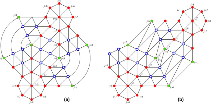
+1 corresponds to the number of x-y planes, the number of points per x-y plane λi can be

Fig. 2 (a) front view and (b) back view of a sample 3D ROI mesh with

π φ

6 1

= and θ 2π 6 1

= . Solid red dots are the initial ellipsoidal contour

calculated as follows:

(

1

)

... 0 −

=

∀i δ , λ0 =λδ−1=1 and δ ≥5:

if δ is odd:

(

2 /

)

× :∀ =1...

(

( −1)/2

)

= λ θ δ

λi i i (5.3)

(

2 /

) (

×

(

−1

)

−

)

:∀ =

(

(

+1

)

/2

) (

... −2

)

= λ θ δ δ δ

λ_i i i (5.4)

if δ is even:

(

2 /

)

× :∀ =1...

(

( −2)/2

)

= λ θ δ

λ_i i i (5.5)

(

2 /

) (

×

(

−1

)

−

)

:∀ =

(

/2

) (

... −2

)

= λ θ δ δ δ

λ_i i i (5.6)

A minimum of five x-y planes is chosen as anything lower does not produce a 3D mesh fit for our purpose. See Fig. 2 for illustration.

C. 3D Snake

The basic snake equation is as follows:

( )

( )

( )

(

)

∫

+ +

= α s E_cont β s E_curv γ s E_img ds

ε (6)

where Econt, Ecurv and Eimg represent the energy for

the continuity, smoothness and edge attraction of the active contours respectively, while the three parameters α , β and γ control the sensitivity of each corresponding property. In the discrete case where the contour is replaced by a chain of N snake points p1, p2, …, pN , the equation becomes:

∑

= × + × + × = N i i img i curv i

cont E E

E 1

γ β

α

ε (7)

where the three energy terms are:

(

)

2

1

−

− −

= _{i i}

i

cont d p p

E (7.1)

2 1

1 2 +

− − +

= _{i i i}

i

curv p p p

E (7.2)

I

E_imgi =−∇ (7.3)

and d equals the average distance between the pairs

(

pi,pi−1

)

and ∇I is the spatial gradient of the intensity

image I, computed at each point.

A 3×3×3 cubic window centred at each snake point is defined within which the energy functions are locally minimised. Furthermore, instead of having only the two pre- or post-neighbouring points in the planar setting, a n×m matrix Mmn is constructed where n is the number of points in Rsnake and m is the number of neighbouring snake points such that m≤

(

2π/θ

)

. Given again

(

/

)

+1

= π φ

δ corresponds to the number of x-y planes, the number of points per x-y plane λi can be calculated as follows:

(

1

)

... 0 −

=

∀i δ , m0 =mδ−1 =

(

2π/θ

)

and δ ≥5:

if δ is odd:

(

)

(

)

(

)

(

) (

)

⎩ ⎨ ⎧ − + = ∀ − − = ∀ = 2 ... 2 / 1 1 2 / ) 1 ( ... 1 : 6 δ δ δ i i

mi (8.1)

(

1

)

/2 :

4 = −

= i δ

m_i (8.2)

if δ is even:

(

)

(

)

(

)

(

) (

)

⎩ ⎨ ⎧ − + = ∀ − − = ∀ = 2 ... 1 2 / 1 2 / ) 2 ( ... 1 : 6 δ δ δ i i

mi (8.3)

(

)

(

/2 1

) (

... /2

)

:

5 ∀ = δ − δ

= i

mi (8.4)

See Fig. 3 for illustration.

Given this is 3D active contours, we now refer to the three energy terms as surface continuity, surface smoothness, and surface attraction. While the surface attraction energy term Eimgi remains the same for each snake point, the continuity and smooth surface energy terms have to be modified to cater for the 3D snake. To obtain Eimgi , a gradient image cube is created after performing; (1) Gaussian smoothing at order σ which starts large and then gradually decreases as the algorithm progresses through the iterations steps and (2) Sobel edge detection on each image slice at each iteration.

Next, with the surface continuity energy term Econti

specified in (7.1), note that the average distance d does

i=0 i=1 j=5 j=6 j=7 j=8 i=6 j=8 j=7 j=6 j=5 i=2 i=3 j=4 j=3 j=4 j=1 j=1 j=2 _i=4 i=5 i=0 i=1 i=2 j=1 j=2 j=5 j=6 j=7 j=8 i=7 j=2 j=1 j=8 j=7 j=6 j=4 i=3 i=4 i=5 i=6 j=5 j=4 j=3 j=3 (a) (b)

Fig. 3 Sample 3D ROI mesh with θ=₈12π. For solid red dots and blue hollow dots, the number of neighbouring points m=6, whereas the green

not refer to the overall average distance between all snake points and their corresponding neighbouring points as in planar active contouring; it only refers to the average distance between the current snake point and its neighbouring points in a 3D context. That is, the equation now becomes:

(

)

∑

=

− −

= m

j

i j i i i

cont d p M

E

1

2

(8.5)

m M p d

m

j

i j i

i

∑

=

−

= 1

(8.6)

Finally, for the planar smoothness energy term Ecurvi specified in (7.2), instead of calculating the squared sum of the distances between a snake point and its immediate pre- or post-neighbouring points, the sum of the squared distances between each snake point and all of its neighbouring points is calculated for surface smoothness. That is, the equation now becomes:

(

)

∑

=

− =

m

j

i j i i

curv p M

E

1

2

(8.7)

Based on the changes above, Equation (7) can be written as:

(

)

∑∑

∑

= =

=

∇ − ×

+ − ×

+

⎟⎟ ⎟ ⎟ ⎟ ⎟

⎠ ⎞

⎜⎜ ⎜ ⎜ ⎜ ⎜

⎝ ⎛

− − − ×

=

n

i m

j

i j i

i j i m

j

i j i

I M p

M p m

M p

1 1

2

2

1

γ β α

ε (9)

Fig. 4 Bland-Altman graphs of congruency between volumes delineated by our method and the known phantom volume of 61,660 voxels for (a) 50 normal and (b) 90 low-count simulations measured against maximum count values.

Fig. 5 Bland-Altman graphs of congruency between volumes delineated by our method and volumes visually delineated by a practitioner for (a) 50 normal and (b) 35 low-count subjects measured against maximum count values.

Note however, in order to correctly implement the greedy 3D active contours algorithm above, it is crucial to normalise the contribution of each energy term. This can be achieved by dividing the surface continuity and surface smoothness energy terms by corresponding maximum values, and the surface attraction energy term by the norm of the spatial gradient in the w×w×w cubic window in which each snake point can move. Based on the findings from our previous study, we continue to use the parameter settings of α =1, β =1 and γ =0.75 after comparing our delineated contours against those visually delineated by an experienced practitioner. To prevent the algorithm from entering an endless loop, a maximum of 100 iterations has been set after evaluating the results obtained from the entire dataset.

IV. IMPLEMENTATION AND RESULTS

To ensure validity and comparability of our results, we use the same measure of congruency C expressed in percentages shown below as has been used in our previous studies:

b d

b d

V V

V V C

∪ ∩

= (10)

where Vd is the delineated volume and Vb is the base volume to which it is compared; 0% means no match whereas 100% represents a perfect match. The results are then displayed via Bland-Altman graphs.

With the simulations, congruency is calculated with Vd equal to the volume delineated by our current method and

b

V as the known phantom volume of 61,660 voxels. An

average of 94% congruency was achieved for the set of 50 normal simulations – a 3% decrease from that achieved by dual exponential thresholding alone. For the set of 90 low-count simulations, our current method achieves 85% congruency which is also a 3% decrease from that achieved by thresholding combined with planar active contours. See Fig. 4 for illustration.

For the real subjects, given we have already verified the validity of the volumes visually delineated by the practitioners, while Vd remains as the volume delineated by 3D active contours, Vb is now represented by practitioner delineated volumes. An average of 91% congruency was achieved which is a 5% drop from the 96% congruency achieved by dual exponential thresholding alone. In terms of the set of 35 low-count subjects, mean congruency is almost the same as the 95% obtained by the thresholding-2D snake combination. See Fig. 5 for illustration.

V. DISCUSSION

A. Main Findings

In this paper, we have shown that the combination of dynamic dual exponential thresholding with 3D active contours continue to deliver an overall congruency of 90% when comparing the delineated volumes against known-volume simulations and subjects visually delineated by practitioners. See Fig. 6 for illustration.

The slight decrease in congruency for normal and low-count subjects is due to overall decrease in the delineated volumes. Given the basis of comparison is thresholding alone, this indicates that the subsequent 3D snake has either successfully removed false lung tissues that are not visually recognisable, or has aggressively removed true lung regions. Examination of the results for normal and low-count simulations also shows that the delineated volumes are less than the known phantom volume. This confirms the cause in performance degradation to be over-aggressiveness in 3D snake delineation.

B. Future Work

Based on the results, it is clear that future work is required to identify the cause of the 3D snake’s

over-aggressiveness in contour delineation. Either existing method need to be adjusted and/or additional energy term(s) may be introduced to specifically cater for 3D implementation. From a dataset perspective, phantoms of known volumes with introduced defect(s) that are similar to those in subject scans with “hotspots” or irregular contours induced by other cardiopulmonary disorders are also desirable for direct verification of our methods developed thus far.

VI. CONCLUSION

We have successfully developed a hybrid method of dynamic thresholding and 3D active contours in delineating SPECT lung contours for PE diagnosis, which is also suitable for the detection of other cardiopulmonary disorders. While evaluation against our previous methods of dynamic thresholding alone and subsequent coupling with planar active contours on similar Monte Carlo simulations and real subject scans revealed delineation of true lung tissues in some cases, overall congruency is still at a very satisfactory 90%. In general, the method detailed in this report provides an accurate and solid foundation for true 3D SPECT lung delineation.

ACKNOWLEDGMENT

We would like to thank the physicians and staff at the Royal North Shore Hospital, Australia for the provision of original datasets and medical guidance.

REFERENCES

[1] T. M. Morell, “Pulmonary embolism,” British Medical Journal, vol. 2, pp. 579-584, 1963.

[2] J. J. Cross, P. M. Kemp, C. G. Walsh et al., “A randomized trial of spiral CT and ventilation perfusion scintigraphy for the diagnosis of pulmonary embolism,” Clinical Radiology, vol. 53, no. 3, pp. 177-82, 1998.

[3] D. M. Howarth, L. Lan, P. A. Thomas et al., “99mTc technegas ventilation and perfusion lung scintigraphy for the diagnosis of pulmonary embolus,” Journal of Nuclear Medicine., vol. 40, no. 4, pp. 579-84, 1999.

[4] A. Gottschalk, H. D. Sostman, R. E. Coleman et al., “Ventilation-perfusion scintigraphy in the PIOPED study. Part I. Data collection and tabulation,” Journal of Nuclear Medicine, vol. 37, no. 7, pp. 1109-1118, 1993.

[5] A. Gottschalk, H. D. Sostman, R. E. Coleman et al., “Ventilation-perfusion scintigraphy in the PIOPED study. Part II. Evaluation of the scintigraphic criteria and interpretations,” Journal of Nuclear Medicine, vol. 34, no. 7, pp. 1119-1126, 1993.

SPECT in the artificially embolized pig,” J Nucl Med, vol. 43, no. 5, pp. 640-7., 2002.

[7] M. Bajc, C. Olsson, B. Olsson et al., “Diagnostic evaluation of planar and tomographic ventilation/perfusion lung images in patients with suspected pulmonary emboli,” Clin Physiol Funct Imaging, vol. 24, pp. 249-256, 2004.

[8] J. Palmer, U. Bitzen, B. Jonson et al., “Comprehensive ventilation/perfusion SPECT,” J Nucl Med, vol. 42, no. 8, pp. 1288-94., 2001.

[9] A. Wang, and H. Yan, “A new automated lung delineation method for SPECT PE diagnosis using adaptive dual exponential thresholding,” Intl J Imaging Sys Tech, vol. 17, no. 1, pp. 22-27, 2007.

[10] A. Wang, and H. Yan, “Delineating low-count defective-contour SPECT lung scans for PE diagnosis using adaptive dual exponential thresholding and active contours,” Intl J Imaging Sys Tech, pp. In Press, 2009.

[11] M. Kass, A. Witkin, and D. Terzopoulos, “Snakes: Active Contour Models,” International Journal of Computer Vision (IJCV), vol. 1, no. 4, pp. 321-331, 1988.

[12] G. An, J. Chen, and Z. Wu, “A fast external force model for snake-based image segmentation,” 9th International Conference on Signal Processing, pp. 1128-1131, 2008.

[13] A. K. Mishra, P. Fieguth, and D. A. Clausi, “Accurate boundary localization using dynamic programming on snakes,” 2008 Canadian Conference on Computer and Robot Vision, pp. 261-268, 2008. [14] M. Sakalli, K. M. Lam, and H. Yan, “A faster converging snake

algorithm to local object boundaries,” IEEE Transactions on Image Processing, vol. 15, no. 5, pp. 1182-1191, 2006.

[15] D. J. Williams, and M. Shah, “A fast algorithm for active contours and curvature estimation,” CVGIP: Image Understanding, vol. 55, no. 1, pp. 14-26, 1992.

[16] L. Ji, and H. Yan, “Robust topology-adaptive snakes for image segmentation,” 2001 International Conference on Image Processing, vol. 2, pp. 797-800, 2006.

[17] T. McInerney, and D. Terzopoulos, “Topologically adaptable snakes,” 5th International Conference on Computer Vision, pp. 840-845, 1995. [18] K. H. Seo, and J. J. Lee, “Object tracking using adaptive color snake

model,” 2003 International Conference on Advanced Intelligent Mechatronics, vol. 2, pp. 1406-1410, 2003.

[19] T. F. Chan, and L. A. Vese, “Active contours without edges,” IEEE Transactions on Image Processing, vol. 10, no. 2, pp. 266-277, 2001. [20] L. D. Cohen, and I. Cohen, “Finite-element methods for active

contour models and balloons for 2-D and 3-D images,” IEEE Transactions on Pattern Analysis and Machine Intelligence, vol. 15, no. 11, pp. 1131-1147, 1993.

[21] Y. B. Hou, and Y. Xiao, “Active snake algorithm on the edge detection for gallstone ultrasound images,” 9th International Conference on Signal Processing, pp. 474-477, 2008.

[22] G. Sundaramoorthi, J. D. Jackson, and A. Yezzi, “Tracking with Sobolev Active Contours,” 2006 Conference on Computer Vision and Pattern Recognition, vol. 1, pp. 674-680, 2006.

[23] G. Sundaramoorthi, A. Yezzi, and A. C. Mennucci, “Coarse-to-fine segmentation and tracking using Sobolev active contours,” IEEE Transactions on Pattern Analysis and Machine Intelligence, vol. 30, no. 5, pp. 851-864, 2008.

[24] J. Liang, G. Ding, and Y. Wu, “Segmentation of the left ventricle from cardiac MR images based on radial GVF snake,” International Conference on BioMedical Engineering and Informatics, vol. 2, pp. 238-242, 2008.

[25] H. P. Ng, K. W. C. Foong, S. H. Ong et al., “Medical image segmentation using feature-based GVF snake,” 29th Annual International Conference on the IEEE, pp. 800-803, 2007.

[26] T. Shimada, L. Wang, and M. Saito, “Auto-extraction of brain region from MR image by using snake controled by neural network,” 22nd Annual International Conference of the IEEE, vol. 4, pp. 3177-3179, 2000.

[27] J. Tang, S. Millington, S. T. Acton et al., “Surface extraction and thickness measurement of the articular cartilage from MR images using directional gradient vector flow snakes,” IEEE Transactions on Biomedical Engineering, vol. 53, no. 5, pp. 896-907, 2006.

[28] W. Wang, L. Ma, and L. Yang, “Liver contour extraction using modified snake with morphological multiscale gradients,” International Conference on Computer Science and Software Engineering, vol. 6, pp. 117-120, 2008.

[29] P. J. Yim, and D. J. Foran, “Volumetry of hepatic metastases in computed tomography using the watershed and active contour algorithms,” 16th IEEE Symposium Computer-Based Medical Systems, pp. 329-335, 2003.

[30] H. Cai, X. Xu, J. Lu et al., “Shape-constrained repulsive snake method to segment and track neurons in 3D microscopy images,” 3rd

IEEE International Symposium on Biomedical Imaging: Nano to Macro, pp. 538-541, 2006.

[31] M. Xiao, S. Xia, and S. Wang, “Geometric active contour model with color and intensity priors for medical image segmentation,” 27th Annual International Conference of the Engineering in Medicine and Biology Society, pp. 6496-6499, 2005.

[32] M. Jung, and H. Kim, “Snaking across 3D meshes,” 12th Pacific Conference on Computer Graphics and Applications, pp. 87-93, 2004.

[33] J. Ahlberg, “Active contours in three dimensions,” Master Thesis, Linkopings University, Sweden, 1996.