250
SEASONAL AVERAGE FLOW
IN RÂUL NEGRU HYDROGRAPHIC BASIN
VIGH MELINDA 1
ABSTRACT. Seasonal average flow in Râul Negru hydrographic basin. The Râul Negru hydrographic basin is a well individualised physical-geographical unit inside the Braşov Depression. The flow is controlled by six hydrometric stations placed on the main river and on two important tributaries. The data base for seasonal flow analysis contains the discharges from 1950-2012. The results of data analysis show that there significant space-time differences between multiannual seasonal averages. Some interesting conclusions can be obtained by comparing abundant and scarce periods. Flow analysis was made using seasonal charts Q = f(T). The similarities come from the basin’s relative homogeneity, and the differences from flow’s evolution and trend. Flow variation is analysed using variation coefficient. In some cases appear significant Cv values differences. Also, Cv values trends are analysed according to basins’ average altitude.
Keywords: Seasonal flow, evolution and trend, altitude differences.
1. INTRODUCTION
Braşov Depression is the biggest unit from the line of depressions that separate the volcanic and the crystalline schist mountainous ranges of the Eastern Carpathians. As a complex physical – geographical entity, it presents a remarkable diversity of genetic factors and flow influences.
The Râul Negru hydrographic basin expands north – south towards the eastern part of the depression, forming a rectangle. The basin’s watershed includes the highest peaks of the Bodoc, Nemira, Vrancea and Întorsurii mountains. The mountainous and depression footsteps are even developed. The mountainous and piedmont areas present high slopes in contrast with the almost plain depression.
The basin’s area is 2320 km2, and the hydrographic network’s density is 0.7 km/km2. The main collector, with a length of 88 km, diagonally crosses the basin’s rectangle. It’s most important tributaries are Caşin, on right, and Covasna, on left.
The main genetic factors are measured at two meteorological stations: Lăcăuţ – in the mountainous area and Târgu Secuiesc – in the depression. The rainfall regime presents maximum values in spring, even though the richest rainfall month is July (173 mm at Lăcăuț, 85 mm at Târgu Secuiesc). Autumn and winter are scarce periods. The monthly minimums present differences: October at Lăcăuţ (40 mm) and December at Târgu Secuiesc (15 mm) (Vigh, 2014). The summer is
1
251
relatively chill. The negative temperatures period lasts five months in the mountains and three months at Târgu Secuiesc, where temperature inversions are frequent.
The flow’s space – time repartition is influenced by the basin’s enclosed character, relief steps development, density and river network characteristic, etc. (Ujvari, 1972).
2. DATA BASE AND METHOD
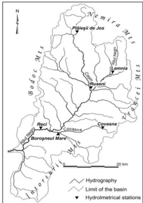
The analysed data come from six hydrometric stations, two on Râul Negru River (Lemnia, Reci), Caşin (Ruseni, Plăieşii de Jos), respectively Covasna (Covasna, Boroşneul Mare) (fig.1.).
From the six stations, three controls the mountainous area, and the others are closing stations, near the main confluences. The analysed period is 1950 – 2012, with some data series being extended for data homogeneity.
The analysis is based on statistical data processing and discharge variation charts interpretation at the six hydrometric stations. The variation coefficients were calculated and average altitude correlations were made (Table 1). The evaluations refer to flow’s time and space evolutions, expressed in absolute and relative values.
Fig.1. Râul Negruhydrographic basin
Table 1. Morphometric data of basin’s hydrometric station
River Hydrometric
station Area
Average altitude
Total length
Lenght down
km2 m km km
Râul Negru Lemnia 101 892 57.2 30.8
Râul Negru Reci 1698 760 80.9 7.1
Caşin Plăieşii de Jos 85.0 954 21.6 32.4
Caşin Ruseni 476 830 51.7 2.3
Covasna Covasna 31.0 1150 10.0 18.0
252
3. MULTINANUAL SEASONAL FLOW EVOLUTION
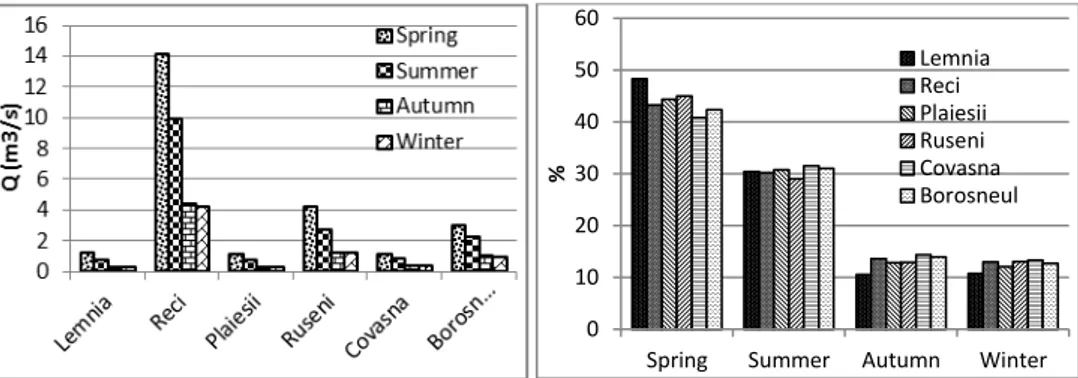
The seasonal discharges’ average values analysis at the six hydrometric stations show a clear domination of spring flow. Next is summer flow. Autumn and winter present scarce flows, with very close discharge values at all stations.
The differences are highlighted also by the seasonal discharge ratio analysis. The spring/summer ratio oscillates between 1.37 (at Boroşneul Mare) and 1.55 (at Ruseni). The spring/autumn and spring/winter ratios are close, with high values, above 3.0. The highest values appear at Ruseni, and the smallest at Boroşneul Mare.
The autumn/winter ratio values are very close to the unit (0.99 – 1.10) and express flow’s regularity in these seasons. As logic, in all cases, the Reci values places between the other two.
Fig. 2. Seasonal variability of flow in absolute and relative values
in Râul Râul Negru Catchement
From the relative values can be observed that at all stations, spring flow exceeds 40% of the total annual flow. At Lemnia, it is close to half (48%). The summer flow is more uniform, with all values very close to 30%. The percentages at Lemnia Station in autumn and winter are at their minimum, little below 10%. The flow at the other stations is higher, between 12 – 14% (Fig. 2.).
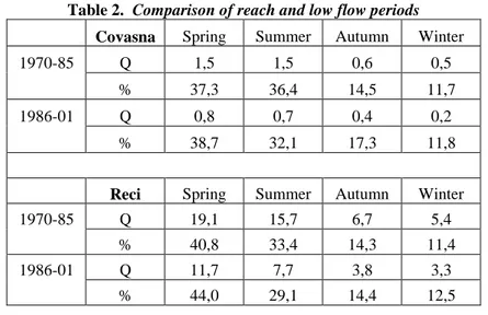
The multiannual average values differentiation can be made comparative, between high flow (1970 – 1985) and low flow periods (1986 – 2001), both including 16 years. For this comparison there have been chosen the stations with extreme average altitudes: Covasna and Reci (mean altitudes: 1150 m, respectively 760 m).
In Table 2 it can be observed that between 1970 – 1985, the spring flow percentage at Covasna is smaller than at Reci (37.3 %, respectively 40.8 %). In summer, the ratio reverses: 36.4 % Covasna, 33.4 % Reci. In autumn and winter, the flow’s relative values are very similar at the two stations.
The low flow period ratios maintain the same laws in spring (38.7 % Covasna, 44.0 % Reci) and summer (32.1 % Covasna, 29.1 % Reci). Obvious differences are observed in the other seasons. The difference in autumn is much
0 10 20 30 40 50 60
Spring Summer Autumn Winter
%
253
higher (17.3 % at Covasna, 14.4 % at Reci) than that in the high flow period. The ratio is even reversed in winter time: the percentage at Covasna is smaller (11.8%) than that at Reci (12.5%).
Table 2. Comparison of reach and low flow periods
Covasna Spring Summer Autumn Winter
1970-85 Q 1,5 1,5 0,6 0,5
% 37,3 36,4 14,5 11,7
1986-01 Q 0,8 0,7 0,4 0,2
% 38,7 32,1 17,3 11,8
Reci Spring Summer Autumn Winter
1970-85 Q 19,1 15,7 6,7 5,4
% 40,8 33,4 14,3 11,4
1986-01 Q 11,7 7,7 3,8 3,3
% 44,0 29,1 14,4 12,5
4. SEASONAL FLOW EVOLUTION BETWEEN 1950 AND 2012
For seasonal flow’s annual values analysis has been chosen two hydrometric stations with extreme average altitude – Covasna and Reci.
There can be observed some evident logical similarities, due to stations’ placement in the same hydrographic basin. The differences are caused by the different altitudes, conditioning flow genesis, and also by the basin’s influences on Reci Station.
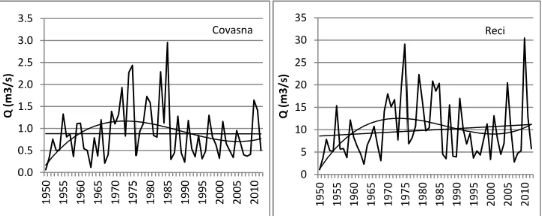
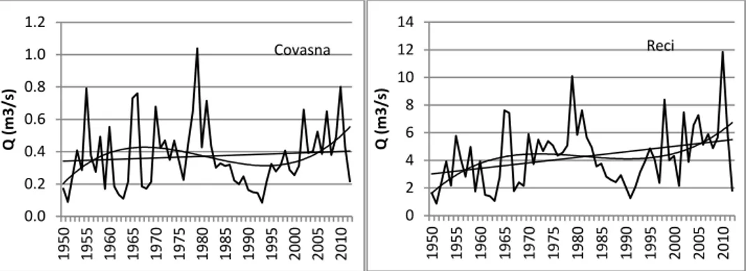
4.1. Spring
The two charts present similar allures, excepting for 1995 – 2005, when the data evolution at Covasna Station is more uniform than that at Reci Station.
Fig. 3. Spring discharge’s evolution (linear and polynomial trend)
0.0 0.5 1.0 1.5 2.0 2.5 3.0 3.5
195
0
195
5
196
0
196
5
197
0
197
5
198
0
198
5
199
0
199
5
200
0
200
5
201
0
Q (m
3/
s)
Covasna
0 10 20 30 40 50
195
0
195
5
196
0
196
5
197
0
197
5
198
0
198
5
199
0
199
5
200
0
200
5
201
0
Q (m
3/
s)
254
The linear trends are contrary – decrease at Covasna, increase at Reci. The 3th degree polynomial oscillations are similar, but the inflexions are more powerful at Covasna Station (Fig. 3).
4.2. Summer
Charts allure presents more evident differences than those in spring, especially in the second part of the analysed period. In this period, the oscillations at Covasna Station are smaller. The linear trend presents stability at Covasna and increase at Reci. The 3th degree polynomial oscillations are much closer than in spring time (Fig. 4).
Fig. 4. Summer discharge’s evolution (linear and polynomial trend)
4.3. Autumn
The variations are less similar due to local rainfalls’ nature that influences autumn minimum flow. Oscillations amplitude is higher at Covasna. The linear trends are also increasing and with similar slopes. Also, the 3th degree polynomial oscillations present high similarities (Fig. 5).
Fig.5. Autumn discharge’s evolution (linear and polynomial trend)
255 4.4. Winter
The two charts highlight, with a strong resembling, the stability of flow genetic factors during winter time. The two stations’ variation curves almost overlap. The inflexions are more powerful at Covasna station (Fig. 6).
Fig. 6. Winter discharge’s evolution (linear and polynomial trend)
5. SEASONAL FLOW VARIATION
The variation coefficient (Cv) expresses how the physical – geographical factors influences flow forming and evolution. Even though the hydrometric stations from Râul Negru basin present relative evident factors’ homogeneity, the Cv values are sometimes with well differences.
The spatial analysis highlights the hydrographic basin’s homogeneity. The Cv values are relatively uniform at all hydrometric stations. But during autumn time the differences are greater. The autumn Cv is much greater than those from the other seasons at Plăieşii de Jos (0.78), Ruseni (0.71) and Boroşneul Mare stations (0.66). At Reci station, the value is the smallest (Cv = 0.42) due to the diminishing effect caused by basin’s high area. The seasonal values at Lemnia station are higher than at other stations, excepting during spring time. The maximum Cv difference between Lemnia (0.53) and other stations (0.30 – 0.35) can be observed during winter time.
Cv values are the highest in autumn. During this season, the highest Cv values can be observed at different stations (0.42 at Reci, 0.78 at Plăieşii de Jos). The Cv values at all stations in the other seasons vary between 0.3 – 0.4. The exception is Lemnia Station during summer and winter time. The most obvious variation coefficients uniformity can be observed during spring time, with a maximum difference of only 0.08 (Fig. 7).
It can be highlighted that the Cv values of Râul Negru, Caşin and Covasna rivers upstream stations are higher than those from downstream in all seasons, representing an obvious law for flow characteristics. There is also an exception: Covasna River during autumn time.
0.0 0.2 0.4 0.6 0.8 1.0 1.2
195
0
195
5
196
0
196
5
197
0
197
5
198
0
198
5
199
0
199
5
200
0
200
5
201
0
Q (m
3/
s)
Covasna
0 2 4 6 8 10 12 14
195
0
195
5
196
0
196
5
197
0
197
5
198
0
198
5
199
0
199
5
200
0
200
5
201
0
Q (m
3/
s)
256
Fig. 7. Cv’s spatial and temporal variability in Râul Râul Negru Catchement
5.1. Cv’s variation in altitude
The Cv values present obvious differences also in the relation with basins’ average altitude. The values increase – law like – with the altitude, excepting in autumn time. The increase slopes are relatively similar. The strongest correlation appears during summer (R2 = 0.85).
Fig. 8. Correlations between altitude (Hmed) and Cv in spring and summer
in Râul Râul Negru Catchement
Fig. 9. Correlations between altitude (Hmed) and Cv in autumn and winter
in Râul Râul Negru Catchement
0 0.1 0.2 0.3 0.4 0.5 0.6 0.7 0.8
0.9 Spring
Summer Autumn Winter
0 0.1 0.2 0.3 0.4 0.5 0.6 0.7 0.8 0.9
Spring Summer Autumn Winter
Lemnia Reci Plaiesii
Ruseni Covasna Borosneul
600 700 800 900 1000 1100 1200
0.3 0.35 0.4
600 700 800 900 1000 1100 1200
0.3 0.35 0.4
600 700 800 900 1000 1100 1200
0.3 0.4 0.5 0.6 0.7 0.8 0.9 600
700 800 900 1000 1100 1200
0.25 0.3 0.35
Hmed
Cv
Hmed
Cv
Hmed
Cv
Hmed
Cv
257
During autumn time, the exceptions previous presented are highlighted in correlation with altitude. If analysing separately each river we can be observed that variation law is not respected on Covasna River.
The relationship between Cv and mail altitude of catchment areas facilitate the territorial generalization of the flow variations (Sorocovschi, Pandi, 2002).
6. CONCLUSIONS
The Râu Negru hydrographic basin presents an obvious homogeneity of seasonal flow. The local influence factors –firstly basins’ altitude and size - cause differences of flow characteristics. This is highlighted by the seasonal average values evaluation at multiannual level, but also by evolutions’ interpretation in the analysed period. These conclusions are highlighted by the flow variation coefficients. The most affected hydrographic basin by the local factors is Covasna River.
REFERENCES
1. Sorocovschi V., Pandi G. (2002), Characteristics of river flow in the
Transylvanian Basin, in Development and Application of Computer Techniques to
Environmental Studies, IX, WIT Press, Southampton, UK, 489-498. 2. Ujvari I. (1972), Geografia apelor României, Edit. Academiei, București