www.j-sens-sens-syst.net/3/281/2014/ doi:10.5194/jsss-3-281-2014
© Author(s) 2014. CC Attribution 3.0 License.
Data fusion of surface normals and point coordinates for
deflectometric measurements
B. Komander1, D. Lorenz1, M. Fischer2, M. Petz2, and R. Tutsch2
1TU Braunschweig, Institut für Analysis und Algebra, Braunschweig, Germany 2TU Braunschweig, Institut für Produktionsmesstechnik, Braunschweig, Germany
Correspondence to:B. Komander ([email protected])
Received: 30 July 2014 – Revised: 27 October 2014 – Accepted: 27 October 2014 – Published: 17 November 2014
Abstract. Measuring specular surfaces can be realized by means of deflectometric measurement systems with at least two reference planes as proposed by Petz and Tutsch (2004). The results are the point coordinates and the normal direction of each valid measurement point. The typical evaluation strategy for continuous surfaces involves an integration or regularization of the measured normals. This method yields smooth results of the surface with deviations in the nanometer range but it is sensitive to systematic deviations. The measured point coordinates are robust against systematic deviations but the noise level is in the order of micrometers. As an alternative evaluation strategy a data-fusion process that combines both the normal direction and the point coor-dinates has been developed. A linear fitting technique is proposed to increase the accuracy of the point coordinate measurements by forming an objective functional as the mean squared misfit of the gradients with respect to the point coordinates on the one hand and to the normals on the other hand. Moreover, a constraint on the maximal change of the coordinate measurements is added to the optimization problem. To minimize to objective under the constraint a projected gradient method is used. The results show that the proposed method is able to adjust the point coordinate measurement to the measured normals and hence decrease the spatial noise level by more than an order of magnitude.
1 Introduction and measurement principle
The combination of close range photogrammetry and struc-tured illumination is well established in the field of three-dimensional measurements of diffusely reflecting surfaces. The so-called fringe projection technique is based on the tri-angulation principle and makes use of at least one electronic camera and one projector. By means of structured illumina-tion, which especially involves phase shifting techniques, the surface under test is optically coded. Based on this spatial coding, the camera images can be evaluated in a way that de-livers a three-dimensional object point for each image pixel. This fringe projection technique depends on the optical imaging of the surface under test onto the image sensor of the camera. This requires a minimum amount of diffusely scattered light from the surface. For reflecting surfaces the amount of diffusely scattered light is very low – in the ideal case there should be no scattered light at all. Reflecting sur-faces therefore are not directly visible, but their presence can
affect the propagation of light in a characteristic way (Tutsch et al., 2011).
Figure 1.Ambiguity of determination of position and orientation of a mirror element in deflectometry (Tutsch et al., 2011).
Figure 2.Principle of an enhanced deflectometric approach using two reference pattern positions (Tutsch et al., 2011).
This ambiguity can only be resolved by additional infor-mation. For instance assumptions can be made concerning the properties of the mirror surface. Then the surface can be reconstructed by means of regularization (Werling et al., 2009). However, the parameters of this reconstruction pro-cess have to be determined by other means, such as approx-imation or additional measurements for at least one point on the surface (Li et al., 2012).
Petz and Ritter (2011), Petz and Tutsch (2004), and Petz (2006) therefore proposed an enhanced deflectometric ap-proach, shown in Fig. 2, that solves the ambiguity discussed for the basic approach. The enhanced approach uses at least two different positions of the reference pattern, which can easily be realized by moving the reference structure with a linear stage. With this approach not only the camera defines a unique ray for each image point, but also the information
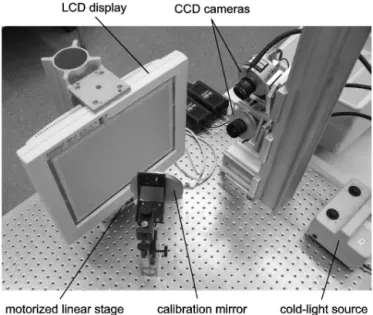
Figure 3.Setup for deflectometric measurements according to the enhanced approach shown in Fig. 2 (Petz, 2006).
from the spatially coded reference patterns delivers an un-ambiguous ray. The intersection of these two rays defines the location of the object point. In addition to the three-dimensional position of the object point also the surface nor-mal in that point can be determined, as for the reflective sur-face the law of reflection must be valid.
A technical realization of the approach illustrated in Fig. 2 can be seen in Fig. 3 (Petz, 2006). As reference structure a common LCD-TFT display is used. The absolute two-dimensional spatial coding of the display area is accom-plished by a combination of phase shifting techniques and a heterodyne approach for deconvolution. The display is mounted onto a motorized linear stage and can thus be moved to various positions during the measurement process. The ob-ject under test will be mounted in the position where the fig-ure shows a calibration mirror, so that the camera observes a mirror image of the LCD display.
As mentioned above, the enhanced deflectometric ap-proach directly delivers three-dimensional coordinates of the observed surface points. Thus there is no need for surface re-construction by means of regularization or integration of the surface slope. However, a closer investigation of the mea-surement data reveals that the direct meamea-surement of coordi-nates is more sensitive to noise than the measurement of the surface normals. In earlier evaluations Petz (2006) has shown that the noise of the measured surface is approximately 3 or-ders of magnitude higher for the direct coordinate measure-ment than it is for the reconstruction based on the integration of the surface slopes.
coordinates determined by triangulation and the observed surface normals. A correspondent approach is the subject of the present paper.
2 Notation and data type
In this paper the Euclidean norm k · konR3 will be used.
Vectors v will be written in italic, bold letters and matri-ces M in bold, capital letters. Scalars c will be written in italic letters. A matrix A, when of dimensionm×n×3, is of form A=(Ax,Ay,Az)withAx,Ay,Az matrices of di-mensionm×n. The vector in theith row and the jth col-umn of Ais denoted with the lowercase, italic, bold letter vi,j =(vxi,j, vyi,j, vzi,j)T ∈R3with itsx,yandzcoordinates.
If any vectorwor matrixAis corresponding tomi,j it will
be written aswi,j orAi,j.
Furthermore, vec(A) is the vector which contains the entries of A∈Rm×n column wise, i.e., vec(A)=
a1,1, a1,2, . . ., am,1, am,2, . . ., am,n T
.
The type of data set being worked with is the result of a deflectometric measurement process as described ear-lier in Sect. 1. After postprocessing the data set contains a matrix P=(Px,Py,Pz) of measured point coordinates to-gether with its information of neighborhood and a matrix N=(Nx,Ny,Nz)of measured normal vectors. The normal vectorsni,j are corresponding to the point coordinatespi,j.
If some measurement point did not yield a valid measure-ment, the corresponding entries in P and N will be unde-fined. Hence, each point coordinate has at most eight neigh-bors, i.e., the eight neighborhood. Point coordinates can have fewer neighbors because of invalid measurements and also at the boundary of the measured object.
3 Objective functional for data fusion
As mentioned in Sect. 1 the accuracy of the normal vectors is approximately 3 orders of magnitude higher than the accu-racy of the measured point coordinates. The purpose of this section is to combine both measured data sets with the objec-tive to get consistent data.
To that end an objective functional will be defined that will fuse the data in a process of optimization. According to the measurement process, it is known that thex and they coor-dinates of the point coorcoor-dinates are more trustworthy com-pared to thezcoordinates. Hence, the objective is to adjust the zcoordinate with respect to the orientation of the mea-sured surface.
The first idea is to take a look at the normal vectors. For every measured point coordinate a calculated normal can be defined by the cross product with two neighboring point co-ordinates. Then the normals can be compared by minimiz-ing the mean squared misfit of the measured and the calcu-lated normals. However, this objective functional leads to an optimization problem which is nonlinear with respect to the
zcoordinate. This is because the mapping from the point co-ordinates to the normals is highly nonlinear. This kind of op-timization problem is surely solvable, but costly in realiza-tion.
By rethinking about information of surface orientation be-side normal vectors, gradient vectors come to mind. Gradi-ents carry the same information about the surface structure as normals. Hence, gradients can be calculated separately with respect to each measured normal and to thezcoordinates of each point coordinate.
Thus, an objective functional can be formed as the mean squared misfit of two kinds of calculated gradients. On the one hand, gradients calculated with respect to the normal vectors and, on the other hand, to the point coordinates. With this approach a quadratic objective functional will be ob-tained.
First the gradient vectorg corresponding to the normal vectors is formed by rearranging the vectors. The firstmn
rows ofgare the partial derivatives of thezcoordinate with respect to thex coordinate and the secondmnrows are the partial derivatives with respect to they coordinate. Thus,g is given by
g= ∇Pz=
−Nx/Nz −Ny/Nz
,
and is of dimension 2mn.
Next the gradient with respect to the point coordinates will be calculated. In order to do that, all neighbors in the eight neighborhood of one point coordinate pi,j, for all
i=1,2, . . ., mandj =1,2, . . ., n, will be located, and build the vectorsv1, . . .,v8frompi,j to its neighbors. The vectors v1, . . .,v8have form
v1=
pxi−1,j−1−pxi,j pyi
−1,j−1−p
y i,j ! , .. .
v8=
pxi
+1,j+1−p
x i,j
pyi+1,j+1−pyi,j
!
.
The point coordinatepi,j with its possible neighbors and the vectorsvk,k=1, . . .,8, are shown in Fig. 4. Note that the
grid defined by the point coordinates is usually not regular. On the one hand the directional derivatives ofpi,j in di-rection to its neighbors can be calculated withv1, . . .,v8 as
follows:
∂vkp
z i,j=v
T
k · ∇pzi,j fork=1, . . .,8. (1)
pi−1,j−1
pi−1,j
pi−1,j+1
pi,j−1
pi,j
pi,j+1
pi+1,j−1
pi+1,j
pi+1,j+1
v1 v2
v3
v4
v5
v6 v7 v8
Figure 4.Neighborhood ofpi,jwith vectorsv1, . . .,v8pointing to all direct neighbors ofpi,j.
needed. It can happen that a point coordinate has fewer than eight neighbors, e.g., at boundary points, so that Vi,j has a smaller number of rows.
On the other hand, the directional derivatives in direction of the neighboring points can be calculated by taking the dif-ferences of thezcoordinates of the neighbors ofpi,jandpi,j itself:
∂v1p
z i,j =p
z
i−1,j−1−p
z i,j,
.. . ∂v8p
z i,j =p
z
i+1,j+1−p
z
i,j. (2)
Putting both Eqs. (1) and (2) for the directional derivatives together, the result is a linear system for∇pzi,j.
Vi,j· ∇pzi,j
=
1 0 0 0 −1 0 0 0 0
0 1 0 0 −1 0 0 0 0
0 0 1 0 −1 0 0 0 0
0 0 0 1 −1 0 0 0 0
0 0 0 0 −1 1 0 0 0
0 0 0 0 −1 0 1 0 0
0 0 0 0 −1 0 0 1 0
0 0 0 0 −1 0 0 0 1
·
piz−1,j−1 pzi
−1,j
piz
−1,j+1
pzi,j−1 pi,jz pzi,j
+1
piz
+1,j−1
pzi+1,j piz+1,j+1
= C· zi,j
The least-squares solution of this overdetermined system for the partial derivatives∇pzi,j is given by
∇pzi,j =
∇xpi,jz
∇ypi,jz
=(Vi,j)+·C·zi,j,
with (Vi,j)+ the pseudo inverse of Vi,j. The matrix
Di,j =(Vi,j)+·Cis the calculated difference matrix of the point coordinatepi,j.
Since the objective is not to calculate the partial deriva-tives separately but to calculate all in one, the entries of each difference matrixDi,j can be written in the proper row and column of a matrixD, which contains all differences for the partial derivatives with respect tox in its firstmnrows, and all differences for the partial derivatives with respect toyin the secondmnrows. SoDis of dimension 2mn×mn. Note that since one point coordinate has at most eight direct neigh-bors, Dwill be a sparse matrix with at most nine nonzero entries per row.
In that way, an objective functional is given as the misfit of the gradients corresponding to the point coordinates and to the normals,
F (Pz)=1
2
g−D·vec(Pz)2,
which will be minimized with respect toPz. The objective functionalF is quadratic in the vectorizedzcoordinates of the points.
Note that the gradient vectorgand the difference matrix Dhave only to be calculated once at the beginning of the process.
4 Linear fitting with steepest descent method
The objective functional was formed in Sect. 3 and it is quadratic inPz. In this section the focus goes to the mea-sured data and the optimization process itself.
An optimalPz corresponding to thex andy coordinates can easily be found by shifting thezcoordinates. Since the point coordinates are given from a deflectometric measure-ment process, the z coordinates cannot be shifted without considering the original position of the measured point coor-dinates and the occurring measurement uncertainties. Hence, the points can only be shifted in a given maximal range.
So the estimated accuracy of the coordinate measurement is used to add a constraint to the optimization problem on the maximal change of the measured points. We assume that the point coordinates are disturbed by noise that follows a Gaus-sian distribution in thezdirection with known varianceσ. Hence, the distribution of the sum of all squared distances in thezdirection follows from a chi-squared distribution with the number of degrees of freedom equal to the numberN
Therefore, with objective functional
F (Pz)=12kg−D·vec(Pz)k2, the optimization prob-lem becomes
minPzF (Pz) s.t Pz−ePz2≤δ.
In order to minimize the objective functional under the constraint, a projected gradient method will be used. There-fore, the search direction for the optimum is given by the negative gradient ofF, which is
−∇F (Pz)= −DT D·vec(Pz)−g,
and, hence, the update for each optimization stepkwith re-spect to the optimization constraint is
Pzk+1=ProjB Pzk−τk· ∇F (P z k)
,
withτkthe step size for the iterationk.
The projection of the point coordinatesPzk onto the setB
is given by ProjB Pzk=
Pzk ,kPz−Pzkk2≤δ
Pzk−1− √
δ
kPzk−Pzk
Pz−Pzk ,kPz−Pzkk2> δ.
Now, a sensible choice of the step size τk is to be made.
By observing the objective functionalF, it can be seen that a convex quadratic problem is to be solved.
The valid step size is
τ = k ∇F (P
z)
k2 kD· ∇F (Pz)k2.
The step size with respect to the gradient ofFatPzkhas to be calculated for each stepk.
Putting all results together, the data-fusion algorithm is as follows.
AlgorithmData-Fusion
Input: Point coordinatesP, normalsN Output: Fittedz-coordinateP˜z
Calculateg,D,∇F
Letǫ >0,k=0,P˜z0=Pz while
P˜
z k+1−P˜
z k > ǫdo
Calculateτk= k∇F(P˜
z
k)k2 kD·∇F(P˜zk)k2 ˜
Pzk+1=ProjB
˜ Pzk−τ
E∇F(P˜z k)
Calculate∇F(P˜zk+1)
k←k+1 end while
5 Experimental results and conclusions
To verify the feasibility of the algorithm, a MATLAB im-plementation of the algorithm has been created. Two sets of
measurement results were used. On the one hand a plane mir-ror and on the other hand a spherical mirmir-ror. In the first case all normal directions of the point coordinates are almost the same, since the measured object is plane. But, a calculation of normals with respect to the measured point coordinates leads to deviations of up to 20◦at some points. With the sec-ond data set similar results in deviations are observed. Since problems can occur during data fusion, further examinations of the data type itself will be done.
5.1 Implementation
In practice, a point coordinate at the boundary of the mea-sured object will have fewer neighbors than eight. Also, point coordinates within the object can have fewer neighbors, e.g., if the measured object has a hole within, has scratches or if some coordinate points could not be measured.
Thus, when the matrixVi,j is formed, there can be en-tries that are not defined and soVi,j (cf. Sect. 3) will have a smaller number of rows. Thus, the matricesCi,j andDi,j and the vectorzi,j will also be smaller during the calculation of the gradient ofpzi,j. In this case, all rows and columns corresponding to the undefined point coordinates have to be deleted.
After calculatingDi,j, the deleted rows and columns of the matrix will be reinserted by writing zeros in the proper row and column, thereby acquiring its original size of 2×8. For insertion, zeros were chosen, because these entries should not and will not be changed during the calculation process. After that the entries ofDi,j can be written within the matrixD.
The matrixDis a sparse matrix, since one point coordinate has at most eight direct neighbors. This matrix is of dimen-sion 2m×n, the firstmrows are corresponding to the partial derivatives with respect tox, the second to the partial deriva-tives with respect toy. The principal diagonal of the firstm
rows and of the secondmrows ofDhas entries correspond-ing to the point coordinatepzi,j and so on. So the entries of each matrixDi,j can be saved in vectors, which can be writ-ten on the diagonals ofD.
5.2 Results
Different data sets were used for the tests. Here, results of the data-fusion process will be shown in direct comparison of the data before and after the calculation. The comparison will be shown by two different measured objects. These objects are a plane reference mirror and a spherical reference mirror.
In Fig. 5 the logarithm of the value of the objective func-tional for both measured objects is shown. In both semi-logarithmic plots it can be seen that the value is falling even by 1000 iteration steps.
0 200 400 600 800 1000 10−2
10−1 100 101 102 103
Iteration
log of functional value
Iteration number w.r.t the logarithm of functional value
Plane mirror Spherical mirror
Figure 5.Logarithm of functional value during iteration for a mea-sured plane reference mirror (lower curve) and for the spherical ref-erence mirror (upper curve).
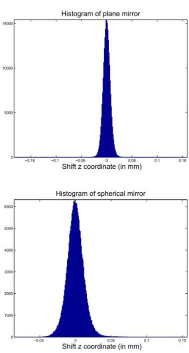
newzcoordinate after data fusion in Fig. 6. It turns out that the histograms are approximately Gaussian and, since our data-fusion model in fact produces consistent data of point coordinates and normals, this verifies a posteriori that the as-sumption of a Gaussian distribution was valid.
In Fig. 7 the gradients of the measured plane and mea-sured spherical reference mirror were plotted. The two plots on the left-hand side show the gradients of the plane mirror before and after the data-fusion process. The two plots on the right-hand side show the same for the spherical mirror. In every plot of this figure the gradients with respect to the measured normals are given in red and the calculated gradi-ents with respect to the point coordinates are given in green. As one can see, the measured gradients all are pointing al-most in the same direction, which is reasonable because the two measured objects did not have any visible jumps on the surface. The calculated gradients before data fusion other-wise differ considerably from the calculated ones. After data fusion the gradients with respect to the fitted point coordi-nates were calculated. On each of the right-hand side plots it can be seen that the new calculated gradients lie on the mea-sured gradients. Hence, the data-fusion process leads to same information of the orientation of the measured surface.
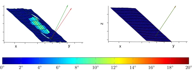
In Fig. 8, the point coordinates before and after data fusion are shown. The surface is colored according to the deviation of the angle between the measured normal and the normal calculated with respect to the point coordinates before and after the optimization process. The color bar is given in de-grees.
Before data fusion, the error between the normal vectors on the surface defined by the point coordinates and the mea-sured normal vectors was up to 20◦ at some coordinates.
−0.15 −0.1 −0.05 0 0.05 0.1 0.15 0
5000 10000 15000
Histogram of plane mirror
Shift z coordinate (in mm)
−0.05 0 0.05 0.1 0.15
0 1000 2000 3000 4000 5000 6000
Histogram of spherical mirror
Shift z coordinate (in mm)
Figure 6.Top panel: residuum of the measuredzcoordinate and
thezcoordinate after data fusion in the plane reference mirror case. Bottom panel: residuum of the measuredzcoordinate and thez co-ordinate after data fusion in the spherical reference mirror case.
After optimization the maximal error was below 1◦in all co-ordinates.
−27 −26.8 −26.6 −26.4 6.2
6.4 6.6 6.8 7 7.2 7.4 7.6
Gradients before data fusion
−27 −26.8 −26.6 −26.4 6.2
6.4 6.6 6.8 7 7.2 7.4 7.6
Gradients after data fusion Gradients of the plane mirror
−5 −4.5 −4 22.5
23 23.5 24 24.5 25
Gradients before data fusion
−5 −4.5 −4 22.5
23 23.5 24 24.5
Gradients after data fusion Gradients of the spherical mirror
Figure 7.Clipped area of plane and spherical mirror gradients before and after the data-fusion process with 1000 iterations. Measured gradients in red, calculated gradients from the point coordinates in green.
y x
z
y x
z
Extract of the plane mirror with normals
0
◦2
◦4
◦6
◦8
◦10
◦12
◦14
◦16
◦18
◦20
◦Figure 8.Left: measured point coordinates. Right: point coordinates after optimization. The red vector is a measured normal, the green a calculated normal. The color encodes the error between calculated normals and measured normals in degrees.
5.3 Conclusions
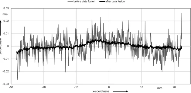
In this paper a novel evaluation approach for a deflectometric measurement has been developed. The results of such a mea-surement, when carried out with multiple reference planes and active triangulation of the incident and reflected light rays, are the three-dimensional point coordinates and normal directions for each valid pixel of the camera. Due to the lo-cal and absolute measurement, the point coordinates are very robust against systematic deviations but with stochastic devi-ations in the order of 10 µm. However, the commonly applied
-0.03 -0.02 -0.01 0 0.01 0.02 0.03
-30 -20 -10 0 10 20
x-coordinate Flatness deviation of plane mirror
before data fusion after data fusion
mm
mm
z
-coordinate
Figure 9.Flatness deviation of one row of the plane mirror before and after data fusion.
Appendix A
A list of all the important variables used.
B=
n
Pz−ePz2≤δ
o The sphere with radiusδaround the measuredzcoordinatePz.
C Matrix.
Di,j=(Vi,j)+·C Difference matrixcorresponding to the point coordinatepi,j. D Difference matrix summarized from alldifference matricesDi,j. δ Tolerance value for shiftingdistance of the point coordinates.
F Pz Objective functionalwith respect to thezcoordinates of the measured points. g Gradient with respect to thezcoordinates of the points.
N Measured normal vectors.
Nx,Ny,Nz Thex,y,zcoordinates of the measurednormal vectors.
P Measured point coordinates.
Px,Py,Pz Thex,y,zcoordinates of the measured point coordinates. ProjB(X) The projection of the setXof point coordinates into the sphereB. vk The vectors which point from a pointcoordinatepi,j to its neighbors. Vi,j Matrix containing all vectorsvk.
Vi,j
+
Edited by: U. Schmid
Reviewed by: two anonymous referees
References
Li, W., Sandner, M., Gesierich, A., and Burke, J.: Absolute optical surface measurement with deflectometry, in: Proc. SPIE 8494, Interferometry XVI: Applications, 84940G, 13 September, 2012. Petz, M.: Rasterreflexions-Photogrammetrie – Ein neues Verfahren zur geometrischen Messung spiegelnder Oberflächen. Disser-tation, Technische Universität Braunschweig, 2006, Schriften-reihe des Instituts für Produktionsmesstechnik, Band 1, Aachen, Shaker, ISBN 3-8322-4944-3, 2006.
Petz, M. and Ritter, R.: Reflection grating method for 3D measure-ment of reflecting surfaces, in: Proc. SPIE Vol. 4399 (2001) – Optical Measurement for Industrial Inspection II: Applications in Production Engineering, edited by: Höfling, R., Jüptner, W., and Kujawinska, M., 35–41, 2011.
Petz, M. and Tutsch, R.: Rasterreflexions-Photogrammetrie zur Messung spiegelnder Oberflächen, tm – Technisches Messen, Heft 71, 389–397, 2004.
Tutsch, R., Petz, M., and Fischer, M.: Optical three-dimensional metrology with structured illumination, Opt. Eng., 50, 101507–101507-10, 2011.