Mocha: a framework to characterize and compare mobility

MOCHA: UM FRAMEWORK PARA

JAVIER JESUS MEDINA DIAZ

MOCHA: UM FRAMEWORK PARA

CARACTERIZAR E COMPARAR TRACES DE

MOBILIDADE

Dissertação apresentada ao Programa de Pós-Graduação em Ciência da Computação do Instituto de Ciências Exatas da Univer-sidade Federal de Minas Gerais como req-uisito parcial para a obtenção do grau de Mestre em Ciência da Computação.

Orientador: Pedro Olmo Stancioli Vaz de Melo

Coorientador: Antonio Alfredo Ferreira Loureiro

JAVIER JESUS MEDINA DIAZ

MOCHA: A FRAMEWORK TO CHARACTERIZE

AND COMPARE MOBILITY TRACES

Dissertation presented to the Graduate Program in Computer Science of the Fed-eral University of Minas Gerais in partial fulfillment of the requirements for the de-gree of Master in Computer Science.

Advisor: Pedro Olmo Stancioli Vaz de Melo

Co-Advisor: Antonio Alfredo Ferreira Loureiro

© 2015, Javier Jesus Medina Diaz.

Todos os direitos reservados

Ficha catalográfica elaborada pela Biblioteca do ICEx - UFMG

Medina Diaz, Javier Jesus.

M491m MOCHA: a framework to characterize and compare mobility traces / Javier Jesus Medina Diaz. — Belo Horizonte, 2015. xxv, 63 f. : il. ; 29cm.

Dissertação (Mestrado) - Universidade Federal de Minas Gerais Departamento de Ciência da Computação.

Orientador: Pedro Olmo Stancioli Vaz de Melo Coorientador: Antônio Alfredo Ferreira Loureiro.

1. Computação - Teses. 2. Redes de computadores - Teses. 3. Roteamento (Administração de redes de computadores) – Teses. I. Orientador. II. Coorientador. III. Título.

Agradecimentos

Primeiramente gostaria de agradecer a Deus, por todas as graças, dons e virtudes concedidas ao longo desta jornada e da minha vida.

Ao meu pai, Gustavo, por todos os conselhos e debates que contribuíram para a minha formação e a deste trabalho. Obrigado por me mostrar através do teu exemplo que nenhuma carga é pesada quando acreditamos no propósito daquilo que estamos fazendo. À minha mãe, Maira, pelo apoio incondicional em todas as minhas decisões e pelo conforto nos momentos mais difíceis. Agradeço também às minhas irmãs, Mariana e Andreina, e a toda à minha família que, mesmo na distância, se fez presente a todo momento.

Obrigado à minha amiga Sthéfanni, por todas as conversas, risadas e situações inusitadas que a nossa amizade nos proporcionou durante esta etapa da minha vida. Ao meu amigo Khalil, pela confiança, pelo constante apoio e por todos os momentos resultantes da nossa convivência diária em Belo Horizonte. À Jocelyn, por sempre estar disposta a ouvir as minhas mais loucas teorias e principalmente por incentivá-las. Aos meus amigos Lucas e Diego por apoiar constantemente meu trabalho e me manterem sempre motivado.

Quero agradecer a todas as pessoas que me acolheram em Belo Horizonte e me fizeram sentir em casa desde o momento em que cheguei, especialmente ao Daniel, à Isadora, sua família e ao Marcos Martins. Agradeço também aos meus colegas de mestrado, Alessandro e Rodrigo Borges, pelos conselhos e pelo apoio em todos os momentos que precisei. Agradeço ao Rodrigo Maués, por me mostrar a resiliência de uma amizade e como o trabalho em equipe sempre pode nos levar mais longe.

“You can’t connect the dots looking forward; you can only connect them looking backwards. So you have to trust that the dots will somehow connect in your future.”

Resumo

A avaliação de algoritmos em MANETs utilizando simulação é fortemente dependente da representação precisa do cenário de mobilidade, ou seja, o modelo de mobilidade e/ou os traces utilizados na simulação devem refletir a realidade da forma mais fiel possível. Existem inúmeros traces na literatura que são utilizados como benchmark

para validar modelos de mobilidade, geradores e soluções para redes sem fio. Além disso, considerando a heterogeneidade dos datasets reais de mobilidade que estão pub-licamente disponíveis é crucial, se não necessário, entender as diferenças e semelhanças entre eles e as suas características. Este trabalho propõe o MOCHA (MObility CHarac-terization Framework), um framework que extrai, classifica e compara propriedades de mobilidade baseado na suas distribuições marginais. Estas propriedades contemplam diferentes aspectos da mobilidade humana e são divididas em três categorias: sociais,

espaciais etemporais. MOCHA é composto por três módulos: um parser, um extrator

e um classificador. O parser é responsável por converter qualquer trace de mobilidade em um formato padrão que possa ser interpretador pelo MOCHA. Oextrator é respon-sável por extrair até 11 propriedades de mobilidade do trace no formato padrão. Por último, o classificador analisa a distribuição marginal de cada propriedade, as separa em cabeça ecauda, e as classifica de acordo com acauda. Uma vez que o MOCHA ex-traiu e classificou cada propriedade, é possível observar as semelhanças entre diferentes

datasets utilizando um algoritmo k-means e fazendo uma Análise de Componentes Principais (PCA). MOCHA foi validado utilizando 13 traces reais que são conhecidos na literatura. Além disso, a validação contou com 18 traces sintéticos gerados com ferramentas conhecidas na literatura. Ao comparar traces reais e sintéticos mostrou-se como os geradores de mobilidade considerados falham em reproduzir cenários realistas e como a metodologia utilizada pelo MOCHA é mais elegante que a dos seus predeces-sores e mais completa, pois considera todos os passos desde a conversão de um trace

de mobilidade, até a classificação das propriedades de mobilidade.

Abstract

The evaluation of mobile network algorithms via simulation is strongly dependent of the accurate representation of the mobility scenario. i.e., the mobility models and/or traces used in simulation should reflect reality as much as possible. There are numerous traces in the literature that are commonly used as benchmark to validate mobility mod-els, generators and wireless networking solutions. Thus, considering the heterogeneity of the real mobility datasets that are publicly available, it is crucial, if not necessary, to understand the di_fferences and similarities among them and also their characteris-tics. In this work we propose MOCHA, a MObility CHaracterization Framework that extract, classify and compare mobility properties, based on their marginal statistical distribution. These properties cover different aspects of human mobility and can be divided into three categories: social, spatial and temporal. MOCHA is composed by three different modules: a parser, a property extractor and a classifier. The parser is responsible for converting any mobility dataset into a standard form that can be understood by MOCHA. The extractor is responsible for extracting up to 11 mobility properties from the parsed dataset. Finally, the classifier analyzes the marginal statis-tical distribution of each mobility property, splits them into head and tails, and classify them according to the tails. Once that MOCHA extract and classify each property, it is possible to visualize the similarities among di_fferent datasets by using a k-means

algorithm and the Principal Component Analysis method. We validate our proposed framework with 13 real mobility traces that are frequently used as benchmark, in addi-tion to 18 synthetic traces generated by different and well known mobility models. By comparing real and synthetic datasets, our results show how the considered mobility generation tools fail to reproduce realistic scenarios. We also show how MOCHA’s methodology is more elegant than their predecessors and more complete, for consid-ering all the steps from the original trace parsing process to the mobility properties classification.

List of Figures

3.1 All Dartmouth mobility properties analyzed by MOCHA . . . 17

3.2 Empirical distributions for graphical comparison . . . 18

4.1 MOCHA structure . . . 26

5.1 Classification of all properties according to MOCHA . . . 46

5.2 Dartmouth INCO fitting and AIC error . . . 48

5.3 SLAW5 INCO fitting and AIC error . . . 49

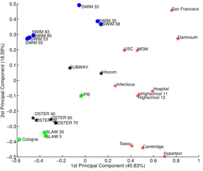
5.4 k-means (k = 2) clustering of all evaluated datasets according to MOCHA using all available properties from all datasets . . . 51

5.5 k-means (k = 4) clustering of all evaluated datasets according to MOCHA using only social properties from all datasets . . . 52

List of Tables

Contents

Agradecimentos xi

Resumo xv

Abstract xvii

List of Figures xix

List of Tables xxi

1 Introduction 1

1.1 Problem . . . 1 1.2 Motivation . . . 2 1.3 Objectives . . . 3 1.4 Contributions . . . 4 1.5 Work organization . . . 4

2 Related Work 5

2.6 Datasets . . . 13

3 Mobility Properties 15

3.1 Discussion . . . 16 3.2 Social properties . . . 16 3.2.1 Inter-contact time (INCO) . . . 18 3.2.2 Contact duration (CODU) . . . 19 3.2.3 Maximum contacts per hour (MAXCON) . . . 19 3.2.4 Encounter regularity (EDGEP) . . . 20 3.2.5 Topological overlap (TOPO) . . . 20 3.3 Spatial properties . . . 21 3.3.1 Radius of gyration (RADG) . . . 21 3.3.2 Travel distance (TRVD) . . . 22 3.4 Temporal properties . . . 22 3.4.1 Visit time (VIST) . . . 22 3.4.2 Travel time (TRVT) . . . 23 3.4.3 Entropy (ENTROPY) . . . 23

4 MOCHA: MObility CHaracterization Framework 25

4.1 Overview . . . 25 4.2 The parser . . . 27 4.2.1 Normalization . . . 28 4.2.2 Raw mobility trace . . . 29 4.2.3 Check-in traces . . . 31 4.2.4 Contact traces . . . 33 4.3 The extractor . . . 34 4.3.1 Social properties . . . 34 4.3.2 Spatial properties . . . 38 4.3.3 Temporal properties . . . 40 4.4 The classifier . . . 42

5 Results 45

5.1 Analysis . . . 45 5.2 Sanity Check . . . 47 5.3 Classification of traces . . . 50

6 Conclusions and Future Work 55

6.1 Conclusions . . . 55

6.2 Future Work . . . 56

Chapter 1

Introduction

1.1

Problem

Mobility traces are receiving considerable attention by researchers in the last years due to the popularization of particular networks such as opportunistic, vehicular and social networks. These traces are mainly used in simulations to reproduce realistic scenarios in which the mobility plays a crucial role in the process of validating an algorithm, technique or protocol [Aschenbruck et al., 2011; Karamshuk et al., 2011; Treurniet, 2014].

A mobility trace is a collection of movements performed by autonomous agents, such as people, animals, vehicles, among others, containing information about this agent. An important class of trace is the one that contains the time and duration of an encounter between two agents, and sometimes their location. Moreover, the traces can describe very large scenarios, such as taxis in a city [Piorkowski et al., 2009], or smaller ones, such as attendees of a conference [Scott et al., 2006], Also, the amount of agents in a trace and the duration of their encounters can also vary significantly, going from dozens of nodes or hours to thousands of nodes and several weeks. Therefore, a key step is to thoroughly understand the properties of such traces to make sure they accurately represent the scenarios targeted by the given algorithm, technique or protocol.

2 Chapter 1. Introduction

et al., 2012; Vastardis and Yang, 2014; Karamshuk et al., 2014; Ekman et al., 2008]. The fact is that mobility traces are the basis of every networking solution based on human mobility.

1.2

Motivation

Mobility can be characterized by several properties [Karamshuk et al., 2011], but most of the generation tools tend to simplify the comparison between generated traces and real traces to a few statistical (and sometimes visual) properties, what harms the process of validating the generative model. Even in the studies that compare mobility traces, there is no standard methodology to perform this comparison. Different types of frameworks have been proposed in the literature without any relation whatsoever among themselves, making difficult to perform a benchmark with tools and datasets that are not considered by the authors.

Bai et al. [2003] use mobility, connectivity and communication performance met-rics to compare traces. Thakur and Helmy [2013] propose a mobility model and a comparison framework with some mobility properties as well as network metrics. Un-fortunately, both studies rely on visual comparison and do not consider how to quan-titatively characterize the scenarios.

On the other hand, some studies [Munjal et al., 2010; Bezerra et al., 2009] use a quantitative approach to analyze mobility models by focusing on statistical curves and parameter fitting. Munjal et al. [2010] propose a model to construct MANET scenarios by defining values for three specific parameters. However, the meaning of each parameter and how to replicate a specific real scenario are questions not answered in that work. Bezerra et al. [2009] propose a methodology to help fitting simulation parameters to desired scenarios, but once again the work fails to explain the nature of each scenario and how to explain why there are similarities between di_fferent datasets. Several studies, such as Aschenbruck et al. [2011], describe the characteristics of both real and synthetic traces. Karamshuk et al. [2011] classify those characteris-tics into three categories: temporal, spatial and social. The characterization of such properties is usually done by the analysis of the probability distribution of the desired property. However, usually this analysis is simply a visual comparison between empir-ical distributions, neglecting any sort of quantitative comparison [Kosta et al., 2014; Lee et al., 2012].

1.3. Objectives 3

compare different scenarios. Furthermore, there is no formal methodology regarding how they should be extracted from each mobility trace. At first sight, this does not look like a real problem because each property has a formal definition, giving us an insight about how to extract it. However, when analyzing real and synthetic datasets, we find several corner cases needing to be considered to guarantee a fair and standard comparison among datasets.

Finally, it is also important to highlight that in the literature each work compares datasets using a specific set of mobility properties, but never all the well-documented properties. By comparing a limited set of properties, it is hard to benchmark datasets between different studies, creating difficulties in determining whether there are actual similarities between scenarios in a standardized and reliable way or not.

1.3

Objectives

The motivation of this work is the establishment of a comparison methodology between mobility scenarios and datasets. Considering this, we propose a MObility CHaracteri-zation Framework (MOCHA) that extracts and compares several mobility properties. First, we propose a taxonomy to classify the different types of mobility traces found in the literature. It is very important to do this because, given the nature of each trace, we need to translate them to a common form in order to guarantee they can be evaluated and compared. Moreover, given a common form, it is possible to extract and compare mobility properties. This will be important for our next goal.

Once we have the entry trace in a parsed form, we use an algorithm to analyze and extract all the considered mobility properties present in it. More specifically, after setting up MOCHA parameters properly, we want to extract quantitative properties from each trace and classify them according to different categories previously identified. The extracted properties represents different aspects of human mobility (such as social ties and regularity [Karamshuk et al., 2011]) and can be used to propose network solutions, especially in ad hoc scenarios.

4 Chapter 1. Introduction

ments of real scenarios, and 13 generated synthetically by well-known models. Our last goal is to categorize these traces using Principal Component Analysis (PCA) to determine whether different traces can be considered similar in nature.

1.4

Contributions

This work proposes MOCHA, a complete framework to extract, analyze and compare mobility properties available in mobility traces. By doing so, this is the starting point to allow a fair comparison between mobility scenarios in order to help us understand their real similarities and differences. With MOCHA, we offer a detailed comparison between traces, improving our understanding on the similarities and differences among mobility scenarios.

By using PCA to several well-known mobility traces used in literature, we present a simple but yet practical form to visualize the similarity of di_fferent traces using a quantifiable method instead of a visual comparison between arbitrarily selected mobil-ity properties. Some of the traces used in our evaluation are Dartmouth [Henderson et al., 2004], Infocom and Cambridge [Scott et al., 2006], San Francisco [Piorkowski et al., 2009] and synthetic traces generated by popular tools such as SWIM [Kosta et al., 2014], SLAW [Lee et al., 2012] and Working Day Model [Ekman et al., 2008].

1.5

Work organization

Chapter 2

Related Work

2.1

Mobility traces

There are several traces commonly seen as benchmark among human mobility models. They can be divided into di_fferent categories: campus, urban pedestrian, vehicular and conference. The di_fference between these categories is not only the geographic scenario itself, but also the methods used to collect the data and the behavior of the agents in each case. In the next sections, we describe each of these categories in details.

2.1.1

Campus scenario

In the campus category, agents are usually students or professors and their movement is restricted to campus locations. Traces such as Dartmouth [Henderson et al., 2004], USC [jen Hsu and Helmy, 2008], SASSY [Bigwood et al., 2011], UPB [Ciobanu and Dobre, 2012] and Cambridge [Scott et al., 2006] are the most known and used in the literature and commonly used to validate networking solutions [Vaz de Melo et al., 2013; Thakur and Helmy, 2013; Alshanyour and Baroudi, 2008] and generative models [Kosta et al., 2014; Lee et al., 2012; Ekman et al., 2008].

6 Chapter 2. Related Work

Finally, the data collection method used in a campus scenario is usually an asso-ciation/disassociation method with the Wi-Fi routers of the campus itself. Every time an agent connects or disconnects to a router, a log entry is generated with the time of the event, the agent ID and the router ID. However, some traces such as Sassy [Bigwood et al., 2011] and [Ciobanu and Dobre, 2012] use Bluetooth instead of Wi-Fi, increasing the precision but limiting the amount of nodes.

This type of data collection method has as main drawback the problem of con-secutive handovers between nearby routers generating, sometimes, noise in the trace. When analyzed, the trace might pass the idea that an agent is constantly moving be-tween locations when it is actually in a handover zone. Another problem this type of data collection emerges is that the geographical coordinates of each router are not always available to the public, making impossible to estimate the actual distances that a node traveled during the trace collection.

2.1.2

Vehicular scenario

There are also vehicular traces, where the agents are vehicles and streets with specific directions and speed restrictions guide their movement. As examples, we can cite San Francisco Cabs [Piorkowski et al., 2009] and Cologne [Uppoor and Fiore, 2012] traces as the most commonly used [Aschenbruck et al., 2011; Karamshuk et al., 2011; Treurniet, 2014].

In this type of scenario, the velocity and acceleration of the agents is more variable than in a pedestrian scenario [Ekman et al., 2008]. Also, it is important to highlight that the paths used by the agents in a vehicular scenario usually have velocity and direction constraints, which are explored by data dissemination protocols and oppor-tunistic networks [Bai et al., 2003].

The social network of a vehicular scenario usually has a random behavior [Vaz de Melo et al., 2013]. Even when the same agents use the same constrained path between two points, it is highly unlikely that they do that at the same time every day. This type of behavior makes more difficult to encounter the same pair of nodes near each other with a certain regularity, giving the social network of a mobility scenario a more random structure.

2.1. Mobility traces 7

The GPS technology has a major drawback when regarding mobility in urban scenarios despite allowing a constant track of each agent. GPS only works well with a clear line of sight between the device and the GPS satellites. In that case, in a city with high buildings, the precision of a GPS can be compromised and the position of a node can be misplaced to a di_fferent road or street than the one that is being actually used. This type of behavior might present itself as noise in the mobility trace.

2.1.3

Conference scenario

Conference scenarios are a specific type of what we can call an indoor scenario. In the conference category, agents are usually students, professors and other kind of partici-pants of the conference, but the same behavior can be compared to hospitals, schools and other indoor scenarios. The Infocom [Scott et al., 2006] and other traces related to hospital and high school [Isella et al., 2011; Vanhems et al., 2013; Fournet and Barrat, 2014] are examples of such traces.

In conference scenarios, the agents move in a similar way of a campus scenario. However, the duration of the trace and the area where the agents move is usually smaller than in a campus trace. Moreover, there are usually no paths, velocity and direction constraints, meaning that the agents move according to a social and not geographic pattern.

The social network of this type of scenarios strongly depends on the scenario itself. A school, for example, will have a very well defined social network, given that students share a lot of time together and have common friends. However, in the case of an hospital, the social network might be represented mostly by the hospital staff, when the patients will configure a random social network between themselves and the staff [Isella et al., 2011].

The data collection method used in indoor scenarios might vary from Wi-Fi as-sociation/disassociation, as in a campus scenario, to the use of proximity devices to determine when an encounter between two nodes actually occurred. When using prox-imity devices, each agent has a unique radio device representing him/her. Once two devices are within each other range, a log entry is generated with each node ID and the time of the beginning of the contact. The same procedure is repeated once the nodes lost communication with each other.

8 Chapter 2. Related Work

2.2

Synthetic mobility generators

Considering the problem of generating mobility traces, the fundamental step is to observe the characteristics of real scenarios, usually done by extracting their statistical properties and represent them as a probability distribution. Previous analysis, as the ones presented by Chaintreau et al. [2007], Song and Kotz [2007] and Helgason et al. [2014a], also show that the behavior of some statistical properties is common to human mobility independently of the environment [Karagiannis et al., 2010]. Based on such analysis, several tools have been proposed to synthetically generate human mobility, some of them discussed below.

However, here we focus on only three: SWIM, SLAW and WDM. We consider those three tools because they are publicly available and are easy to set up and install, making possible to anyone to reproduce the results presented in this work. Moreover, these generators are very popular and constantly used by researchers to validate net-working solutions [Munjal et al., 2010; Sandulescu et al., 2013; Batabyal and Bhaumik, 2014].

2.2.1

SWIM

Kosta et al. [2014] propose a generator called SWIM (Small World In Motion) to generate synthetic small world scenarios. In SWIM, each node receives a home location and moves around cells, calculating each cell popularity according to the number of nodes present at each location. Until a cell is visited, its popularity to the node is defined as zero. The intuition behind SWIM is that nodes visit with higher probability nearby or popular cells.

SWIM assumes that the time spent between two locations by any node will be always the same. This is based on the fact that agents tend to accomplish short distance jumps on foot and long distance jumps by car or plane. Later in this work, it will be shown when this assumption is in fact valid and in which cases are not.

According to [Kosta et al., 2014], SWIM can successfully reproduce real traces be-havior such as the Cambridge mobility traces [Scott et al., 2006] and Dartmouth [Hen-derson et al., 2004] by comparing three different mobility properties: inter-contact time, contact duration and contacts per node. However, as we show in this work, SWIM fails to model the social regularity present in real traces.

2.2.2

SLAW

2.2. Synthetic mobility generators 9

power-law flights and pause times, heterogeneously bounded mobility areas, truncated power-law inter-contact times and fractal waypoints. They show these premises are intrinsically related, since the validation of one of them tends to generate the behavior expected in some of the others.

Lee et al. [2012] also show that their model successfully fits power-law distribution in properties such as inter-contact time and flight distances using the Akaike test. However, their comparison is performed with traces collected by themselves and are not publicly available. This creates obvious difficulties to benchmark their tool with other real datasets.

The decision algorithm of SLAW agents is strongly based on what they call as

Leas action trip planning, or LAPT. LAPT states that every time agents need to visit more than one location, they choose their next destination primarily based on the shortest distance. Only when all the possible locations are within a specific radius (say 30 meters) the decision criteria is not the distance but the importance of the location itself.

2.2.3

Working Day Model

Finally, Ekman et al. [2008] propose a mobility model called Working Day Model (WDM), which has the purpose of modeling realistically daily routines. To accomplish such modeling, they created separated sub-models to represent the di_fferent parts of human routine: home sub-model, o_ffice sub-model and evening activity sub-model.

They also model different types of mobility such as walking, bus and cars. By assigning to each node a home location and a work location, WDM sets the mobility of each agent according to the time of the day and its specific parameters (e.g., working hours and how often each agent uses a car or a public transportation). For example, by the morning each node goes from home to work using its preferred transportation method (e.g., foot, car or bus) and spends all their working hours moving according to an o_ffice mobility pattern.

Once the working hours finish, each agent decides with a given probability whether it will go back home or to a social meeting with friends using an evening activity mobility model. In the evening activity model, each agent is assigned to a meeting location and, once it arrives, it waits until all friends arrive, too. Then, the whole group start visiting night locations until certain time, when everyone goes back home.

10 Chapter 2. Related Work

datasets properties. Yet, WDM does not clearly evaluate all the statistical mobility properties that can be extracted from generated mobility traces.

2.3

Comparing Mobility Traces

In order to determine whether two or more scenarios are similar, a comparison is needed. This comparison is usually done by extracting properties from each trace and comparing the statistical distribution of their values [Thakur and Helmy, 2013; Bezerra et al., 2009; Bai et al., 2003]. Another common approach is to use network protocols and evaluate the underlying network using metrics such as delay, throughput and overhead to determine if the protocol exhibits a similar performance in both sce-narios [Meghanathan and Milton, 2009; Boldrini et al., 2007]. Several studies compare mobility traces by creating different scenarios in NS-2 [Mccanne et al., 2007] consid-ering parameters such as simulation time, area, number of nodes, transmission range, pause time, traffic rate, etc [Meghanathan and Milton, 2009; Boldrini et al., 2007; Bai et al., 2003].

The compared properties of each study are usually di_fferent. However, even when considering di_fferent comparison parameters and methodologies, most of those studies conclude that mobility affect the performance of opportunistic networks and there are underlying social properties that need to be considered in order to better understand their results.

Munjal et al. [2010] propose a methodology to construct synthetic mobility sce-narios using SLAW [Lee et al., 2012]. By studying carefully the impact of all the configuration parameters of SLAW, they provide models to construct realistic mobility scenarios. However, they do not consider any mobility property during their evaluation such as inter-contact time or contact duration. Thus, they only use network metrics to evaluate their results.

Bezerra et al. [2009] propose a framework to compare mobility models by using mobility properties instead of network metrics. By extracting properties, such as agent speed, acceleration and pause time, they use a fitting method to determine how to set the mobility models parameters in order to imitate real data. They conclude that some mobility models, such asLevy-walk, MMIG and Smooth, have too many param-eters, making very hard to determine in which intervals these parameters can actually generate mobility that resembles real scenarios.

2.4. Mobility-based networking solutions 11

well-known real datasets, such as the ones presented in Section 2.1. Thakur and Helmy [2013] propose COBRA, a mobility model based on communal behavior, and bench-mark it with real datasets using an analysis framework. COBRA compares mobility properties, such as inter-contact times and contact duration, besides network metrics. However, they do not explain how the mobility properties are extracted from each trace. They validate the extracted data through a visual graphical comparison, but neglect any quantitative analysis.

Helgason et al. [2014b] compare pedestrian scenarios generated by Legion Stu-dio [Helgason et al., 2010] using mobility properties, such as inter-contact times, contact duration and path duration. Once the properties are extracted, they compare diff er-ent scenarios by fitting statistical curves using Kolmogorov-Smirnov method. They conclude that the considered properties are not enough to understand exactly why the compared traces are di_fferent and state the need of an extensive suit of bench-mark traces for evaluating mobility in di_fferent environments rather than attempting to derive a one-size-fits-all analytical model for pedestrian mobility.

By proposing MOCHA, our work presents a benchmark framework with 18 well-known real mobility datasets, using more than 10 mobility properties to compare and classify them. Considering its structure, MOCHA focus on understanding the mobility characteristics of each scenario, rather than creating a generic mobility model that suits all scenarios.

2.4

Mobility-based networking solutions

While the previously described studies focus on understanding mobility models and compare them to validate their findings, another line of research focus on developing networking solutions based on mobility analysis. Vaz de Melo et al. [2013] propose RECAST, a strategy used to classify interactions among wireless users based on social regularity and similarity. They also apply their strategy to well-known real datasets and use network metrics to validate it.

12 Chapter 2. Related Work

erties such as flight time and pause time to propose a novel scheduling algorithm for opportunistic networks. They use mobility scenarios generated only from theoretical models, neglecting real mobility traces. Moreover, they validate their results using only network metrics. In the same direction, Alshanyour and Baroudi [2008] evaluate AODV protocol performance.

Finally, mobility-based networking solutions directed to opportunistic scenar-ios [Fischer et al., 2010] and disaster scenarscenar-ios [Aschenbruck et al., 2004] can be found in the literature. However, most of the previously described studies fail to provide a detailed framework that allows a standard comparison among different mobility models or traces. While the authors continue to extract mobility properties in an arbitrary way, it will not be possible to properly benchmark different solutions and reach a com-mon understanding of how social mobility truly affects protocols and other networking solutions.

2.5

Overview

One of the main purposes of mobility traces is to test and validate applications to be used in real scenarios. However, since it is not possible to collect real data from all possible scenarios, simulators are used to approximate the results according to the specific situations where the applications will be implemented. When regarding human mobility, several mobility properties have been studied in order to enable their synthetic reproduction using simulators. However, considering that real scenarios are very heterogeneous, it is really hard to reproduce each possible scenario using only a few parameters.

Simulators like SWIM bet on their simplicity to enable an intuitive form of mobil-ity generation, but they do not consider the fact that human mobilmobil-ity is more complex than the probability of moving far away from home or to a popular location. Consider-ing that, SLAW tries to capture the social behavior within the mobility by introducConsider-ing more parameters and by using the locations (or fractal points) as points of social con-vergence, making possible to the agents to imitate social bounds by meeting large amounts of nodes (and even the same nodes sometimes) at high entropy locations. However, as we show later in this work, SLAW fails to reproduce the social regularity that exists in real datasets.

2.6. Datasets 13

to reproduce a scenario that we do not fully understand? Even with a high set of tunable parameters, how much can we approximate a real scenario with synthetic data if we only rely on a few properties to compare? Moreover, given that the parameter space is very large, it is likely that we generate scenarios with very distinct properties. Thus, a tool to provide a reliable comparison of mobility traces is required.

In summary, the main problem about realistic traces is that they are very het-erogeneous, even when they are collected in similar scenarios such as campus, city and conferences. The mobility nature of the nodes might be different at each case, making difficult to create a mobility model based on them [Song et al., 2010]. In the next chap-ters, we will explain the known mobility properties used in the literature. Moreover, we present MOCHA, a framework that allows us to compare different scenarios, helping us to understand how exactly two scenarios can be considered similar or different.

2.6

Datasets

In this work, we analyze several real and synthetic datasets. Each trace has unique mobility properties, but all of them are composed of a set of agents moving around a limited area. The amount of information collected at each case is related to the duration of each trace. While some of them present data collected during a couple of days, some of them were collected for periods longer than 60 days.

14 Chapter 2. Related Work

Name Agents Duration Reference

Dartmouth 1156 60 days Henderson et al. [2004]

Cambridge 12 6 days Scott et al. [2006]

Sassy 27 79 days Bigwood et al. [2011]

USC 4558 60 days jen Hsu and Helmy [2008]

UPB 35 4 days Ciobanu and Dobre [2012]

Infocom 41 3 days Scott et al. [2006]

Hypertext 113 1 day Isella et al. [2011]

Hospital 75 4 days Vanhems et al. [2013]

Highschool 2011 126 7 days Fournet and Barrat [2014]

Highschool 2012 126 7 days Fournet and Barrat [2014]

Infectious 416 1 day Isella et al. [2011]

San Francisco 551 30 days Piorkowski et al. [2009]

Cologne 700.000 car trips 24 hours Uppoor and Fiore [2012]

Table 2.1. Mobility traces of real scenarios

Trace Agents Duration Reference

Working day model (WDM) 100 agents 15 days Ekman et al. [2008]

SLAW 5 100 agents 15 days Lee et al. [2012]

SLAW 35 100 agents 15 days Lee et al. [2012]

Ostermalm 90 1000 agents 7 days Kouyoumdjieva et al. [2014]

Ostermalm 70 1000 agents 7 days Kouyoumdjieva et al. [2014]

Ostermalm 50 1000 agents 7 days Kouyoumdjieva et al. [2014]

Ostermalm 40 1000 agents 7 days Kouyoumdjieva et al. [2014]

Ostermalm 30 1000 agents 7 days Kouyoumdjieva et al. [2014]

SWIM 88 100 agents 7 days Kosta et al. [2014]

SWIM 85 100 agents 7 days Kosta et al. [2014]

SWIM 83 100 agents 1 day Kosta et al. [2014]

SWIM 58 100 agents 30 days Kosta et al. [2014]

SWIM 55 100 agents 24 hours Kosta et al. [2014]

SWIM 53 100 agents 15 days Kosta et al. [2014]

SWIM 38 100 agents 15 days Kosta et al. [2014]

SWIM 35 100 agents 15 days Kosta et al. [2014]

SWIM 33 100 agents 15 days Kosta et al. [2014]

Chapter 3

Mobility Properties

As previously described in Karamshuk et al. [2011], the statistical properties extracted from mobility traces can be categorized in: social, spatial and temporal properties. De-spite all mobility properties being intrinsically related, we can divide them in categories according to their application regarding networking solutions and social mobility.

Social properties, such asinter-contact time andcontact duration, can be directly related to connectivity. These properties help us to explain how agents connect

among themselves, how long they stay within each other range, how they relate to each other and, consequently, how we can explore these properties to benefit our delivery ratio ordelivery throughput in a real network scenario. It is very useful to understand how long agents interacts with each other, when developing applications that require data transmission or mobility analysis.

Spatial properties, such as radius of gyration and travel distances, are related to

movement, giving us some insights about distances covered by each agent and its

relation to locations. Intuitively, we can affirm that people prefer to go to the bakery nearby their home instead of going to a distant bakery, unless, for instance, the distant one is really popular or has been recommended by a friend. Simulators like SLAW [Lee et al., 2012] exploit this kind of intuition by generating mobility using fractal points, as previously described.

Finally, temporal properties, such as visit time, travel time and location entropy, represent regularity. This regularity reflects the circadian rhythm defining each

16 Chapter 3. Mobility Properties

3.1

Discussion

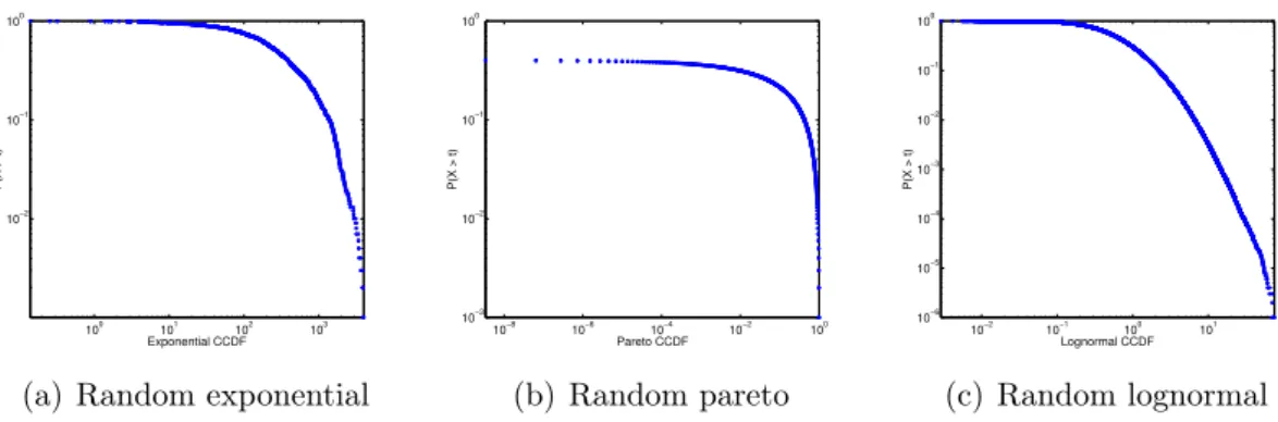
Mobility properties give us insights about how agents behave in different scenarios. This information can be used to reproduce real datasets with synthetic generators. As previously explained in Sections 3.2, 3.3 and 3.4, most of the properties can be modeled as statistical curves and most of them are represented by heavy-tailed distributions. Here, we plot all the statistical distributions using their complementary cumulative distribution function, or CCDF.

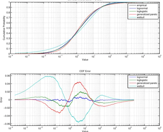
In Figure 3.1, we see all the extracted mobility properties from the Dartmouth dataset. We use this dataset as reference because it is one of the most famous dataset and is commonly used as a benchmark in the literature [Vaz de Melo et al., 2013; Zyba et al., 2011]. We can also observe in Figures 3.2(a), 3.2(b) and 3.2(c) three empirical distributions considered by MOCHA: exponential, pareto and lognormal.

As previously described in Section 1.2, most of the current studies regarding mobility properties rely on a visual comparison of statistical distributions to validate if di_fferent datasets are somehow similar or equivalent. Later in this work, we will show how this visual comparison can be tricky and misleading sometimes, showing why it is important to use a quantitative comparison method instead of a visual matching. Note that several plots in Figure 3.1 seem to be heavy-tailed. However, as we show later, some of the distributions are best fitted by a pareto curve while other are best fitted by a lognormal one. This shows, again, how important it is to perform a quantitative analysis when comparing different mobility scenarios.

3.2

Social properties

In the following, we consider a set of m agents {N1, N2,· · ·, Nm}, each one having a

positionNi(t) = (x, y), i= 1. . . m, as the position (x, y) in the cartesian plane at time t 0. Each scenario has severalencounters between different pairs of nodes. For GPS traces, an encounter betweenNi andNj occurs wheneverdist(i, j)R, wheredist(i, j)

is the Euclidean distance between Ni and Nj and R is the communication radius of

each agent. For traces collected with router association/disassociation, an encounter happens whenNi and Nj are connected to the same access point at the same time. In

this case, the encounter begins at the moment and ends when one of them disconnects. Thus, each scenario is composed of an ordered set of encounters E =

{e1_{, e}2_{,· · ·, e}n_{}, where each encounter e}k _{= {N}

i, Nj, tini, tf in} is composed of the

3.2. Social properties 17

100 105

10−5

100

P(X > t)

(a) Inter-contact time (b) Contact duration

0 48 96 144

0 2 4 6x 10

4

Hour of simulation (x)

MAXCON

(c) Max contacts per hour

10

10

P(X > t)

(d) Topological overlap

10

10

P(X > t)

(e) Edge persistence

10−10

10−5

100

P(X > t)

(f) Radius of gyration

100 105

10−5 100

P(X > t)

(g) Travel distance

100 102

10−5

100

P(X > t)

(h) Travel time

(i) Visit time

10

10

10

P(X > t)

18 Chapter 3. Mobility Properties

100 ₁₀1 ₁₀2 ₁₀3

10−2

10−1

100

Exponential CCDF

P(X > t)

(a) Random exponential

10−8

10−6

10−4

10−2

100

10−3

10−2

10−1

100

Pareto CCDF

P(X > t)

(b) Random pareto

10−2 ₁₀−1 ₁₀0 ₁₀1

10−6

10−5

10−4

10−3

10−2

10−1

100

Lognormal CCDF

P(X > t)

(c) Random lognormal

Figure 3.2. Empirical distributions for graphical comparison

Ei,j = (Ni, Nj, ti, tf) 2 E as the set of all the consecutive encounters between Ni and Nj.

3.2.1

Inter-contact time (INCO)

Inter-contact time can be defined as the time interval between consecutive encounters of a pair of nodes [Kosta et al., 2014]. While inter-contact time is represented by the time between consecutive contacts of the same pair of agents, some authors, such as Helgason et al. [2010], prefer to use a more generic definition called inter-any-contact time, which considers consecutive contacts between any pair of agents. To the purpose of this work, we will use the first definition because it is more popular in the literature. Thus, for a given ordered setEi,j ={e1i,j, e2i,j,· · ·}of encounters between agentsNi and Nj, we compute the inter-contact time between two encounters eki,j and e

k+1

i,j as:

INCOk i,j =t

k+1

ini tkf in.

When considering the statistical representation of this property, we usually obtain a heavy-tailed distribution (such as power-law) [Helgason et al., 2014b]. This intuitively explains that, independently of the encounters duration, most of the nodes do not encounter with each other very frequently [Kosta et al., 2014]. For legibility purposes, we will refer the property as INCO and will use the acronym INCO-D when referring to its statistical behavior (i.e., distribution). We will use this notation for all properties in this work.

3.2. Social properties 19

magnitude, indicating that despite some pairs of agents encountering with each other very frequently, most of them pass long periods without meeting.

3.2.2

Contact duration (CODU)

The definition of the contact duration property is very straightforward. It is the amount of time a pair of agents is located within each other’s communication range without leaving it. In other words, we can define the CODU of an encounter

ek_={N

i, Nj, tini, tf in} as:

CODUk

i,j =tkf in tkini.

This behavior can be observed in Figure 3.1(b).

In an analogous way to INCO, CODU also represents an opportunity to deliver a message in an opportunistic network. However, if INCO gives us an insight about how frequently a message can be delivery, CODU helps us to understand for how long an encounter takes places, i.e., how much data can be transferred during an encounter. The understanding of this property is directly related to the possible output that each agent can transmit while in contact with another agent.

3.2.3

Maximum contacts per hour (MAXCON)

As explained by Song and Kotz [2007] and Ekman et al. [2008], the maximum contacts per hour is the total amount of contacts that occurred at each hour of the considered dataset. Formally, we define MAXCON as:

MAXCONh =Eh ={e= (Ni, Nj, tini, tf in)|(tini > h^tf in < h+ 1)_(tini <= h^tf in >=h)},

where Eh _{is the subset of all encounters between every pair (N}

i, Nj) that occurred

during the hourh, and|Eh|is the sum of those encounters. The set of all the encounters

occurring during a scenario evaluation can be defined as H ={|E1_|,|E2_{|,· · ·}.}

Regarding the statistical behavior of H, we can describe it as a curve with high autocorrelation in 24 h periods [Song and Kotz, 2007; Karamshuk et al., 2014]. The au-tocorrelation can be explained by the daily routine behavior occurring in any scenario in which agents are humans. The statistical representation of H will be described as MAXCON-D and its autocorrelation as MAXCON-Cw wherewis the time window

20 Chapter 3. Mobility Properties

MAXCON is a property that helps us to understand how many contacts occurred during a specific hour. Considering it is aconnectivity property, we observe that it gives us insights about how many different opportunities of sending a message an agent has during each hour of the day and, in which parts of the day, the agent has more (or less) interactions with other agents (e.g., the number of social contacts during the day is usually higher than during the night).

3.2.4

Encounter regularity (EDGEP)

Edge persistence is a complex network metric that maps the regularity of a social relationship [Vaz de Melo et al., 2013]. By considering a set of encounters Ei,j =

(Ni, Nj, ti, tf)2E EDGEPi,j measures the times the encounterek ={Ni, Nj, tini, tf in}

occurred from t0 tot, where0ttmax. Formally, we have:

EDGEPi,j = 1_tPtk=1I[(i,j)∈εk],

whereI[(i,j)∈εk] is an indicator function that assumes the value 1if the encounter ek =

{Ni, Nj, tini, tf in} occurred in εk at time k, and 0 otherwise. For example, if Bob and

Patrick met each other twice during a week their edge persistence will be equal to the number of times they encountered, i.e., 2 divided by the total number of time steps, i.e., 7.

According to [Vaz de Melo et al., 2013], we can expect a heavy tailed distribution when considering the statistical behavior of EDGEP-D. By observing Figure 3.1(e), we observe that there are many EDGEP with low values (i.e., pairs of nodes encountering sporadically) and few high EDGEP values, which represent the most strong social ties. Intuitively we can affirm that an agent tends to encounter more frequently with its friends or acquaintances while random encounters rarely repeat [Vaz de Melo et al., 2013]. The more each pair of nodes encounters in a specific time window, the more probable is to consider a social tie between those nodes. When considering oppor-tunistic scenarios, EDGEP represents how often it will be possible to deliver a message between a specific pair of nodes.

3.2.5

Topological overlap (TOPO)

Another property that gives us insights about the social network of each scenario is the topological overlap. TOPO represents the social overlap existing between each pair of nodes when considering all the encounters in which they participated. First, we consider asN Gi orneighborsi the set of nodes{N1, N2,· · ·, Nm}encountering at least

3.3. Spatial properties 21

TOPOi,j =

|N Gi\N Gj|

|N Gi[N Gj|

.

Analogous to EDGEP-D, TOPO-D also presents a heavy-tailed behavior accord-ing to [Vaz de Melo et al., 2013], as observed in Figure 3.1(d). TOPO-D gives us insights about the social structure of each scenario by quantifying the similarities be-tween agents.

By considering each pair of agents, we observe in Figure 3.1(d) that most of them have few, or even none, common friends, indicating that there is no social tie between them. On other hand, nodes presenting a high TOPO value are more likely to belong to the same communities and have a higher amount of common friends.

When regarding network applications, TOPO is helpful to determine opportuni-ties to deliver messages within communiopportuni-ties. Intuitively it is easier to deliver a message to a member of the same social community than to a complete stranger.

3.3

Spatial properties

3.3.1

Radius of gyration (RADG)

In social mobility, it is common to assume that each agent has a location called home. citeswim defineshome as a randomly and uniformly chosen point over the network area. Ekman et al. [2008] consider it as the starting point of each agent’s daily activities. To the purpose of this work, we will consider home as the most visited place at each agent’s routine and where normally the agent returns at the end of the day.

It is plausible to assume that an agent tends to move to other locations nearby its home in order to attend commitments, buy food, visit friends, etc. There is a mobility property measuring the distance an agent “orbits” around its home and is called radius of gyration. We consider a time-ordered set Li ={l1, l2,· · ·, ln} of locations visited by Ni and Hi as its home. Formally,

RADGk,i=dist(lk, Hi),

where dist(lk)i represents the Euclidean distance between location lk 2 Li and Ni

home Hi. When considering all locations Li, we obtain RADG-D. As observed in

22 Chapter 3. Mobility Properties

3.3.2

Travel distance (TRVD)

When an agent moves from a location to another one, we usually describe that action as a travel, jump or flight [Karamshuk et al., 2011; Ekman et al., 2008]. The travel distance definition is very straightforward. It is the distance traveled between two consecutive locations [Ekman et al., 2008]. Formally, by considering a time-ordered set

Li ={l1, l2,· · ·, ln} of locations visited by Ni we have:

TRVDk,k+1 =dist(lk, lk+1),

where dist(lk, lk+1) is the Euclidean distance between lk and lk−1. When considering

all the travels performed by an agent, we obtain TRVD-D. As can be observed in Fig-ure 3.1(g), TRVD-D presents a heavy-tailed behavior. This behavior indicates that agents perform short distance jumps more often than long distance ones. This obser-vation is according to the least action principle of Maupertuis [1744], and used by Lee et al. [2012] to model SLAW.

TRVD is very related to RADG and the main difference between them is that RADG considers the travel distance according to the nodes’ home, and not the dis-tance between consecutive visited locations. The analysis of these properties helps us to understand how agents move from a place to another one. This information can be ex-ploited, for instance, to improve message dissemination in vehicular and opportunistic networks.

3.4

Temporal properties

3.4.1

Visit time (VIST)

Visit time can be defined as the time spent at each location visited by an agent [Karamshuk et al., 2011]. Considering a time-ordered setVi ={v1, v2,· · ·, vn}of

visitsvk= (lk, tini, tf in), lk being the location visited at momentk, we have:

VISTk =tf in tini.

3.4. Temporal properties 23

3.4.2

Travel time (TRVT)

In an analogous form to the travel distance, we define the travel time TRVT as the time an agent spends moving from one location to the consecutive one. Considering a time-ordered set Vi ={v1, v2,· · ·, vn} of visits vk = (lk, tini, tf in), vk being the location

visited at moment k, we have:

TRVTk,k+1 =tinik+1 tf ink.

Considering all the agent’s visits, we plot TRVT-D in Figure 3.1(h). When com-pared to the travel distance property (described in Section 3.3.1), the statistical be-havior matches the idea that long trips are less frequent, but demand more time to be completed, while short travels are faster and common, i.e., leading to a heavy tail distribution.

3.4.3

Entropy (ENTROPY)

It is known that in mobility scenarios agents develop social ties between themselves and those ties influence the way agents move from one place to another one [Shah and Rathod, 2014; Foroozani et al., 2014; Helgason et al., 2014a]. However, it is possible to state that agents also develop social ties with locations. In real scenarios, people tend to visit more often places that are somehow familiar to them or are visited by their family, friends or acquaintances.

In this work, we define an entropy property, which quantifies the amount of visits each location receives in a specific scenario. By considering a set of locations

L={l1, l2,· · ·} we define:

ENTROPYk =Pi= 1nPk= 1mλ(i, k),

where λ_{(i, k)} is a function representing the number of times agent _Ni visited location

lock,n is the total of agents and m the total of considered locations.

Chapter 4

MOCHA: MObility

CHaracterization Framework

The purpose of this work is to design a framework to extract, analyze and compare mobility properties of different mobility scenarios. To the best of our knowledge, there is no study that analyzes, compares and classifies mobility scenarios in a detailed and broad way as we do in this work.

MOCHA encompasses the most commonly used mobility properties, dividing them into three groups as proposed by Karamshuk et al. [2011]: social, spatial and temporal.

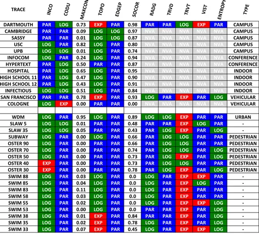
The social properties considered in this framework are: inter-contact time (INCO), contact duration time (CODU), maximum contacts per hour (MAXCON), topological overlap (TOPO), edge persistence (EDGEP) and the social correlation (SOCOR). The spatial properties are: the travel distance (TRVD) and radius of gy-ration (RADG). Finally, the temporal properties are: visit time (VIST), travel time (TRVT) and the locations entropy (ENTROPY). All these properties, but SOCOR were described previously in Chapter 3.

4.1

Overview

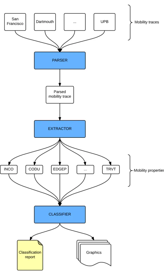
MOCHA is composed of three modules: parser, extractor and classifier. The parser

26 Chapter 4. MOCHA: MObility CHaracterization Framework

4.2. The parser 27

The initial MOCHA entry is a mobility trace collected from a real environment or generated by a synthetic tool. Although these traces may contain any type of information, only a few are mandatory for MOCHA. Thus, the first step is to parse the trace into MOCHA’s format. Once the mobility trace is parsed, we obtain a new trace in a defined form to be analyzed by MOCHA.

After that, the parsed mobility trace is used as input to the extractor. MOCHA’s

extractor generates a file for each considered property with all the extracted entries. Most of the properties are independent of each other and MOCHA allows the extraction of each property individually.

Finally, after all the mobility properties are extracted, MOCHA’s classifier ana-lyzes the data and generates a classification report with the category of each property. MOCHA can also generate graphics for each property according to its type. The graph-ics that MOCHA can generate are: complementary cumulative distribution function (CCDF), cumulative distribution function (CDF) and histogram.

The following sections will explain in detail how each MOCHA module works and which considerations were made along its design in order to be able to consider and analyze different scenarios.

4.2

The parser

In the design of MOCHA, we have to consider the heterogeneous nature of the traces found in the literature [Aschenbruck et al., 2011] and the different forms of data col-lection used regarding human mobility [Aschenbruck et al., 2011; Karamshuk et al., 2011; Treurniet, 2014]. In that direction, the first module of the framework is a parser, responsible for converting any trace to a common (internal) form with all the data needed to extract the statistical properties described in Chapter 3.

This step is important to ensure generality and extensibility of the framework. By using a standard input form, we allow anyone to evaluate a mobility trace with all the benchmarks.

28 Chapter 4. MOCHA: MObility CHaracterization Framework

dataset are described in Table 2.1.

Finally, San Francisco and Cologne are vehicular traces. These traces are pre-sented in different forms related to the way they were collected. Some of them were collected using WLAN connection logs and others by using GPS or iMotes or other proximity detection devices. The di_fferences between these traces are explained in Chapter 2.

Given these traces, we divided them into three categories: raw mobility traces, check-in traces and encounter traces. It is important to highlight that there might be other kinds of traces available, but we have chosen this three types because they are the most popular and almost every other kind of trace can be easily converted to one of them.

Each trace is composed of different entries representing a travel or an encounter that occurred in the considered scenario. By considering these three main types of mobility traces, we propose the utilization of the following common form for the entries in any dataset evaluated by MOCHA in order to maintain the homogeneity of our framework:

Ni Nj tf in tini δt xi yi xj yj,

where Ni and Nj are two distinct agents, tini is the initial time of the encounter, tf in

is the final time of the encounter, δ_t is the encounter duration and _{(x, y)i} and _{(x, y)j}

are Ni and Nj coordinates at the beginning of the encounter.

Our format is based on encounters because they can summarize a wide variety of statistical properties without the need to use too much memory or processing, sim-plifying the framework and the evaluation process. Considering that, we leave to the

parser the responsibility to digest the input data that will be analyzed by the next modules.

4.2.1

Normalization

Before we can explain how the mobility properties are extracted and classified, we need to define the methodology used to convert any mobility trace into MOCHA’s common form. This explanation is important to ensure reproducibility and, thus, the homogeneity of the evaluation. First, it is important to normalize the trace. The trace normalization will ensure the correct evaluation of each dataset and will avoid calculation errors.

4.2. The parser 29

what is the earliest time entry present in the trace and subtract it from all of the time values. To normalize the IDs we create a dictionary and map all the agents to a new ID value between 0 and n, where n is the total amount of distinct nodes minus one. The normalization of the coordinates is similar to the time normalization with one di_fference: it can only be done when the coordinates used on the trace are planar, not geographical. In traces that use GPS coordinates, it is not recommended to do a normalization considering that geographical coordinates are not linear. We will address this scenario later in this work.

Finally, all trace entries must be ordered by time. This ordering is necessary because some mobility properties to be extracted are time-dependent and it is easier to analyze them in an ordered way.

4.2.2

Raw mobility trace

The raw mobility trace is the most generic type of trace that can be found in the literature. It basically informs us the position of each agent in a specific time, but gives us no information about visited locations and social encounters. The most important aspect of this type of trace is the granularity of the time window, since it affects the precision of extracted properties. For example, a 1-second time window will give us a better information about social encounters than a 1-hour or even half-hour time window. However, the smaller the time window is, the more complex the entry process will be. Sometimes, an agent can move very short distances or even stay at the same place for several hours, making unnecessary to constantly track its behavior.

Raw traces are very popular among vehicular traces and even in some synthetic mobility generators such as NS-2 [Mccanne et al., 2007]. The main drawback of this type of trace, besides the difficulty of its processing, it is that we need to infer which locations are visited by each agent. Because raw mobility traces often give us specific coordinates, we need to infer where the social locations are, such as malls, train stations and schools. Considering that our framework is oriented to social mobility, there is no much we can obtain by evaluating the raw mobility only, so we need to use the mobility information to generate encounters and geographic locations instead of only individual coordinates.

30 Chapter 4. MOCHA: MObility CHaracterization Framework

whereNi is the agent’s ID, (x, y)i are the coordinates where the event occurred and t

is the time of the event. It is important to point out that other data might be found in raw mobility traces, such as nodes’ speed, for example, but we will focus on the information used by our method to generate our common trace form.

Assuming that T is the time ordered according to the preprocessing, we will analyze entry-by-entry using a graph G and a matrix M to support the encounter

generation. We also define an encounter criterion stating that an encounter between two nodes occurs every time the Euclidean distance between them is equal or inferior to a thresholdR. This assumption is valid according to how encounters happen in mobile

network, whereRis the radius of communication of each device [Helgason et al., 2014a].

The Euclidean distanced(p, q) is defined as follows:

d(p,q) =d(q,p) =

q

(q1 p1)2+ (q2 p2)2+...+ (qn pn)2 =

q Pn

i=1(qi pi)2,

where p = (p1, p2,· · ·, pn) and q = (q1, q2,· · ·, qn) are two points in the Euclidean n

-space. For notation purposes, we define maxx and maxy as the maximum X and Y

values encountered in the preprocessing step. In order to assist us in the encounter calculation, we have created a grid M of the size of the trace scenario using maxx

and maxy in a way that each cell has a diagonal equal to R. By doing that, we

guarantee that all nodes present at each cell are within the encounter range of each other. Formally, we defineM as:

M =

⇢ ck,l |

✓

0k  maxx

R ◆

^ ✓

0l  maxy

R ◆

,

whereck,l represents a cell in M. After creating the grid, we are ready to process the

trace T. In this stage, we create a new node Ni in G to every node found in T that

has not being already created, and we store the node coordinates at the time of its creation. Considering the coordinates(x, y)i registered at the trace entry, we allocate Ni in its respective cell ck,l wherek =

xi

R and l =

yi R.

OnceNi its allocated to ck,l, we retrieve all nodesNj present in the rangeck−1,l−1

to ck+1,l+1 to verify if the Euclidean distance between Ni and Nj is equal or inferior

to R. If so, we create an edge E(i,j) in G between Ni and Nj, with a value equal to

the timet present in the current evaluated entry of T . We also consider as neighbors, or N Gi, all nodes Nj discovered in this step. If the evaluated entry in the previous

step represents the first occurrence of node Ni in the trace, we consider that N Gi is

empty. However, if there is a previous entry with Ni, it is probable that N Gi is not

empty. Therefore, we need to evaluate if all the previously existent nodes in N Gi are

4.2. The parser 31

the current set of neighbors with the previous one and compute all nodes that are not neighbors anymore.

Once we identify that a node Nk is not a neighbor of Ni anymore, we search

for the edge E(i,k), whose value is equal to the time tp when the encounter between i

and k began, and register a new entry in our log according to the standard proposed previously:

Ni Nk tc tp (tc tp) xi yi xk yk,

whereNi andNk are the nodes IDs,tc is the current entry time,tp is the time when the

edge betweeniandkwas created,(xi, yi)are the currentNicoordinates and(xk, yk)are

the Nk coordinates when the encounter began. By repeating the described procedure

for every entry in T, we can successfully parse a raw mobility trace to our common

form. This process is fully described in Algorithm 4.1.

Algorithm 4.1. Raw mobility trace parser algorithm

# e n t r y = Ni x i y i t i

f o r e n t r y i n T:

i f G. has_node ( Ni ) :

f o r Nk i n n e i g h b o r s ( Ni ) :

i f not e u c l i d e a n ( Ni , Nk) :

g e n e r a t e _ e n t r y ( Ni , Nk , t i , G[ Ni ] [ Nj [ time ] , ( t i -G[ Ni ] [ Nj [ time ] ) , xi , yi , xk , yk ) G. remove_edge ( Ni , Nk)

e l s e:

G. add_node ( Ni )

f o r Nj i n n e i g h b o r s ( Ni ) :

i f e u c l i d e a n ( Ni , Nj ) :

G. add_edge ( Ni , Nj , time = t c )

4.2.3

Check-in traces

32 Chapter 4. MOCHA: MObility CHaracterization Framework

check-in traces give us no information about how long the node stayed there and which locations the node might have visited between consecutive check-ins.

Because of the information gap check-in traces have, we need to infer how the social encounters happen in every location, how long each node stayed in the location, how long they took to travel from a location to another and so on. The usual format of this type of trace is:

Ni li t,

whereNi is the agent’s ID, li is the location’s ID and t is the time of the check-in. It

is important to point out that most of the times there are no geographical coordinates available and only the arrival time is informed. Later on, we will explain how this lack of information affects the property extraction, but, for now, we will focus on the parsing.

Assuming thatT is time ordered according to the preprocessing, we will analyze entry-by-entry using a graphGand a dictionaryL indexed by the location IDs. First, we create a dictionary of locations. For each entry inT we includeNiin the location Li

once a check-in occurs. At the check-in moment, we create an edgeE(i,j) inG between

Ni and all nodes present in Li.

Considering that the checkout time is not provided, we define the values maxt as

the longest duration each node can stay in a specific location and movt as the average

movement time between two locations. If the same node Ni happens to check-in in

another location before the expiration ofmaxt, we create a new log entry for all edges Ei,j with the following format:

Ni Nj (tc movt)tp (tc tp)0 0 0 0,

where Ni and Nj are the nodes IDs, tc is the current entry time minus movt, tp is

the time when the edge between i and j was created and the zeros represent the lack

of information regarding the coordinates of the locations. If the coordinates of the location Li happen to be available, the zeros can be replaced with Lx, Ly, Lx, Ly,

respectively. Otherwise, if maxt is reached before Ni performs another check-in, the

checkout fromLi will be automatically executed creating a new log entry for all edges Ei,j with the same format but the value of tc will be equal to (tp+maxt) instead of

(tc movt). This process is fully described in Algorithm 4.2.

Algorithm 4.2. Check-in mobility trace parser algorithm