Parametric Optimization in WEDM of WC-Co Composite by Neuro-Genetic Technique



Abstract_{—The present work does a multi-objective}

optimization in wire electro-discharge machining (WEDM) of tungsten carbide-cobalt (WC-Co) composite. Optimization was done with the help of a Neuro-Genetic technique which was developed through a combination of a radial basis function network (RBFN) and non-dominated sorting genetic algorithm (NSGAII). Experiments were carried out based on Taguchi design of experiments involving six control factors such as pulse on-time, pulse off-time, peak current, capacitance, gap voltage, and wire feed rate. Cutting speed, surface roughness and kerf width were considered as the measures of performance of the process. The proposed Neuro-Genetic technique was found to be potential in finding alternative optimal input conditions of the process. These optimal solutions may lead to efficient utilization of WEDM in industry.

Index Terms_{— NSGA-II, RBFN, WC-Co, WEDM}

I. INTRODUCTION

ITH the introduction of new hard materials to be machined, super-hard tool materials were developed. Among several super-hard tool materials, cemented carbides, especially WC-Co composites were found to be potential materials to making cutting tools, metal-working tools, mining tools and wear resistance components. This is because of its greater hardness, strength and wears resistance over a wide range of temperatures. WC-Co composite is synthesized by the sintering of WC granules that are held together by Co binders.

Wire electro-discharge machining process was found to be an extremely powerful electro-thermal process for machining WC-Co composites with any intricate shape. This process erodes materials by minute electrical discharges between the wire-electrode (50-300 micron diameter) and the work-piece. Although WEDM was found to be potential for machining WC-Co composites, it has some major limitations particularly while machining this composite. A large difference in melting and evaporation temperatures of it constituents, makes the process unstable [1]. The melting and evaporation temperatures of tungsten

Manuscript received Feb 23, 2011; revised March 25, 2011.

P. Saha* is with the Indian Institute of Technology Patna, Patna-800013, India, Department of Mechanical Engineering (corresponding author, phone: +91-612-2552006; fax: 0612-2277382; (e-mail: [email protected]).

P. Saha is with Indian Institute of Technology Kharagpur, Kharagpur-721302, India, Department of Mechanical Engineering (e-mail: [email protected]).

S. K. Pal is with Indian Institute of Technology Kharagpur, Kharagpur-721302, India, Department of Mechanical Engineering (e-mail: [email protected])

carbide are 28000C and 60000C, respectively while those for Co are 13200C and 27000C, respectively. Therefore, Co gets melted, evaporated and removed by the discharge energy even before the melting of WC. As a result, in absence of a binder (Co) the WC grains may be released without melting and may lead to unstable machining. Unstable machining causes short circuit, arcing etc. Hence, it is quite difficult to model such process by analytical approach based on the physics of this process. There have not been significant research publications till today on processing of these hard WC-Co composite materials by WEDM. Thus, there is non-availability of machining databases for this type of materials. In absence of a database, an appropriate model, capable of predicting machining behavior for a wide range of operating conditions, finds immense utility. Few mathematical models developed so far [2]-[3] relies upon several assumptions to simplify the process and eventually predicts a process performance which is quite far from the reality. In this context, as neural networks are highly flexible modeling tool with the ability to learn the mapping between input and output without knowing a prior relationship between them, they could be used for modeling of such random and complex process. In the present work RBFN was implemented to develop this model.

The authors, in their previous work [4], have already done an extensive parametric study on this material by WEDM. This parametric study reveals that there is not available even a single input condition which can maximize cutting speed and minimize surface roughness or kerf width simultaneously. Therefore, it is a multi-objective optimization problem. In multi-objective optimization, user may require several solutions instead of a single one. These solutions are called Pareto-optimal solutions and they are equally important. Depending upon the requirement of the user, any one of them can be selected. Say for example, in rough cutting, a process engineer must select such an input condition from the Pareto-optimal solutions which can provide a larger cutting speed. This selected input condition may also produce higher kerf width (higher the kerf width, lower will be the dimensional accuracy). But the process engineer is not worried for that as his objective is to maximize cutting speed irrespective of any value of kerf width. Similarly in fine cutting, the selected input condition must be such that it will minimize kerf width irrespective of any value of cutting speed. As NSGA-II works with a population of points, it may capture several solutions which would be required for the multi-objective optimization problem. NSGA-II requires a fitness function which is nothing but a relationship between input and output parameters. As RBFN is making that relationship, hence, it

Parametric Optimization in WEDM of WC-Co

Composite by Neuro-Genetic Technique

P. Saha*, P. Saha, and S. K. Pal

is coupled with NSGA-II, and thus making a Neuro-Genetic technique.

Several attempts have been made to model and optimize the process [5]-[8]. The modeling and optimization techniques, used by the past researchers have some limitations. Say for example, the limitation of regression method is that it may not depict the underlying nonlinear complex relationship between the decision variables and responses. In addition to that it also requires a prior assumption regarding functional relationship (such as linear, quadratic, higher order polynomial and exponential) between input and output decision variables. This paper attempts to map input and output variables of WEDM by RBFN. The RBFN is superior over the back-propagation neural network due to the following reasons: it is less complex, it requires fewer training samples, only one layer of nonlinear elements is sufficient for establishing arbitrary input-output mapping, it requires less training time, and chance of getting local minimal convergence is less [9]. Similarly in optimization, most of the researchers used either simple weighting method, converting multi-objective problem into a single objective or constraint optimization method. The drawback of the simple weighting method is that it is very much sensitive to the weight vectors and needs prior knowledge to the problem. The limitation in constraint optimization technique is that the optimal value of one response is obtained while keeping the other one at a desired value and hence, providing single solution at a time. As in the real world situation user may require different alternatives in decision making; therefore, the above methods need to be solved number of times as the requirement changes. As the wire electro-discharge machining database for WC-Co is not readily available and hence, any attempt to model and optimize the WEDM process parameters would be very much useful to the process engineers.

II. EXPERIMENTATION

In the present research work, a 4-axis CNC WEDM (Make: Electronica Machine Tools Ltd., India, Model: Electra Maxicut) was used for the study. The machine has a transistor controlled RC relaxation circuit and deionized water is used here as a dielectric fluid. This study took WC-Co composite with some alloying elements as the work-piece material. The composition and the physical properties of the work-piece are given in Table I.

TABLEI

COMPOSITION AND PHYSICAL PROPERTIES OF WC-CO COMPOSITE

According to the Taguchi quality design concept a mixed orthogonal array, L32 was used for the experiments. A total of six machining parameters such as pulse on-time, pulse off-time, peak current, capacitance, average gap voltage, and wire feed rate were considered as the controlling factors. Among the six input parameters, one has two levels and the remaining five have four levels. The detailed

machining condition is shown in Table II. After completion of the experiments the performances of the WEDM process were measured by the methods explained in the next section.

TABLEII

MACHINING CONDITION

A. Measurement Procedure

Cutting speed (mm/min): Cutting speed was evaluated under each cutting condition by dividing the cutting length with the required cutting time.

Kerf width (mm): A diagram of kerf width is shown in Fig. 1.

Fig.1. Work-piece showing kerf width

Once the machining was over, each machined surface was cleaned with acetone bath in an ultrasonic cleaner, and kerf width was measured by an optical microscope attached with a micro-hardness tester (Make LECO, Model: M-400-H1) equipped with a digital micrometer.

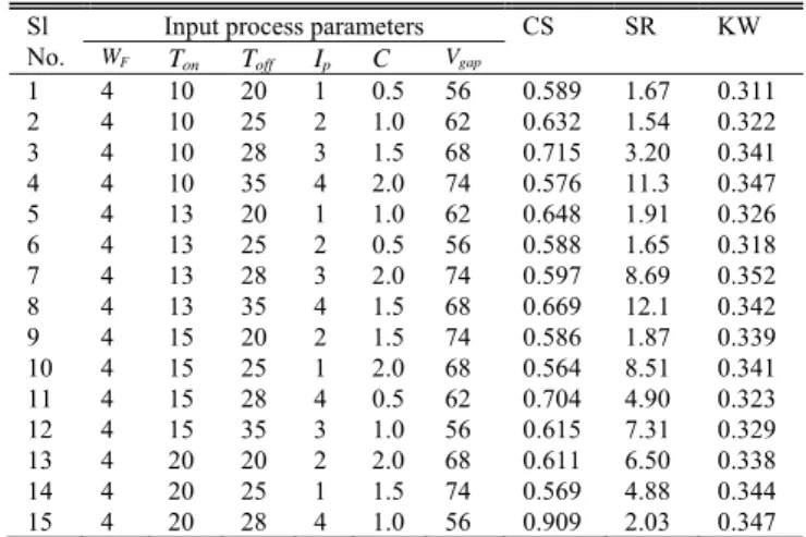
TABLEIII EXPERIMENTAL RESULTS

For each cut, total twelve kerf width measurements have been taken at different positions along the length of the cut

Composition WC 76.5 wt%, Co 11.5 wt%, Alloying elements 12 wt%

Grain size 2.4-2.8 µm Batch hardness 1363-1391 HV30

Process parameter Level Unit

1 2 3 4

Wire feed rate (WF) 4 6 mm/min

Pulse on-time (Ton) 10 13 15 20 μs

Pulse off-time (Toff) 20 25 28 35 μs

Peak current setting (Ip) 1 2 3 4 step

Capacitance (C) 0.5 1 1.5 2 μF Average gap voltage (Vgap) 56 62 68 74 V

Sl No.

Input process parameters CS SR KW

WF Ton Toff Ip C Vgap

and finally, the average of those readings were considered.

Surface roughness (µm): Average surface roughness (Ra)

was measured by SJ-201P Mitutoyo portable roughness tester. Multiple readings were taken for each cut and average was considered. The cut off length and sampling length were been kept as 0.8 and 3 mm, respectively. A total thirty-nine experiments were conducted. Out of that, thirty experimental data were used to train the network and rests were used for validation of the models. Due to limitation of space, only fifteen experimental results are shown in Table III.

III. RBFNBASEDMODELING OF THEPROCESS

A. An Overview of RBFN

RBF networks consist of an input layer, one hidden layer, and an output layer. The hidden layer contains an array of nonlinear radial basis functions, which are generally Gaussian functions. The output of the kth hidden node is obtained by the following expression:

2 exp

-2 2 k =

k ₂

n

exp -2 2

k = 1 k

 



 

 

 

 

 

 

 

 _{ }

 

 

X Ck

X Ck

(1)

where, X_x x_{1 2 3}, ,x ,...,_xl_ is the input vector (also a pattern), _Ck[c_1k,c_2k,...,c_lk] is the center vector of the kth

hidden node having same dimension as that of the input vector, lis the dimension of input and center vector, kis

the Gaussian width of the kth hidden neuron and nis the number of neurons or centers in the hidden layer. _{X Ck}- is the Euclidean distance between input and kth center. The outcome of the jth unit of the output layer is obtained through a linear combination of the nonlinear outputs from the hidden layer and is given by the following expression:

,

n s =_{j k k j}w

k=1 

 (2) where, _{wk j}is the synaptic weight between the kth hidden node and jth output neuron.

It is indeed important to indicate that the performance of the RBFN depends on the centers of the Gaussian functions. Ideally, the centers should represent the whole input data space. Initially the centers are chosen at random. The initial random centers may not partition the whole input space effectively, resulting in poor approximation capability of the RBF network. Therefore, it is very much essential to optimize the initial centers. In the present work, the centers were optimized by two methods. The first method is k-means clustering and the second one is gradient descent.

K-means clustering technique [10]

K-means clustering algorithm partitions the whole input space into some regions and finds the optimal centers of each region, which can represent the input dataset belonging to that region. In this algorithm, P number of l-dimensional input vectors of the training dataset,_Xi, i =1, 2, ...., P, are

partitioned into n number of clusters denoted by _Gk, k = 1, 2, ...., n. It is assumed that at optimal partition, a cost function of dissimilarity measure would be minimized. This cost function is presented by the following expression:

2

1 ,

n Cost function

k i _Gk

 

 

  _   _

 _{ Xi} Xi Ck _, (3)

where, _Gkis the kth cluster group. The optimal center

Ckthat minimizes the cost function is the mean of all input vectors in group k.

1

,

Gk i _Gk

 



C_k X_i

Xi

(4) where,

1

P G_k u_ji

i  

 (5)

where, P is the number of training pattern, and the membership matrix is given by

2 ₂

1,

0,

if for all k j

u ji

otherwise 

    

  

X_i C_j X_i C_k

(6)

Gradient descent technique [11]

K-means clustering technique may achieve a local optimum solution which also depends on the initial choice of the cluster centers. The consequence of the local optimality is that it would never reach to the desired value and causes wasting of computational time. In order to obtain a better result, a gradient descent learning algorithm was implemented. Irrespective of the value of initial centers, the optimal centers could be obtained by this technique. After (p+1)thpattern presentation, the centers are updated by the following expression:

1

1 p

p p

c_ik c_{ik c} p c_ik 

  

  

 (7)

where, c_ikp1is the component of kth center vector after (p+1)th pattern presentation, _cis the learning rate for centers,.  is given by the following equation:

2

1 1 1

1

2 ₁

q _{p p}

p _{t s}

j j

j

   _{ }    _

 

 (8)

where, q is the number of outputs, tp_j1 is the target output of the (p+1)th pattern presentation, sp_j1 is the predicted output of the same pattern. After finding the optimal centers of the Gaussian functions by the two methods, the forward calculation was done. Based on the difference between predicted output and target output, the synaptic weights, connecting the neurons of hidden layer and output layer were updated. This was done by the gradient descent learning algorithm. The synaptic weights were modified by the following expression:

1 1

p E j

p p

w_kj w_{kj w}

p w_kj 

 

   (9)

neuron and jth output neuron, _wis the learning rate for weights and

1

1 1

p

E_{k p p p}

s

j j k

p W_kj

t 



 _{ }

 



 

 

  . The training will be

stopped when mean square error (MSE) for training will reach to a threshold value. The MSE is calculated by the following expression:

2 1

2 _{1 1}

P _{p p}

MSE _j s_j

P_{p j} t

q

   

 

 

 

  (10) B. Development and Validation of Models

The dataset as listed in Table III was used to train the networks. In order to do a fare comparison between the models, a same value of MSE for training was used for both the models. Here it is 0.004. Once the optimal center locations were obtained, the synaptic weights were updated by gradient descent learning algorithm. In case of RBFN with k-means, the network parameters such as n, 2 and

w

 were obtained by trial and error method. This was carried out by varying the MSE for testing against these parameters. It was found that a 6-24-3 architecture yields better results while2and _w were kept as 0.3 and 0.5, respectively. On the other hand, in case of RBFN with gradient descent technique, the optimal center locations along with other network parameters were obtained by gradient descent method. Here also a 6-24-3 architecture yields better prediction whilec,(learning rate for Gaussian width) and _w were kept as 0.5, 0.6 and 0.3, respectively.

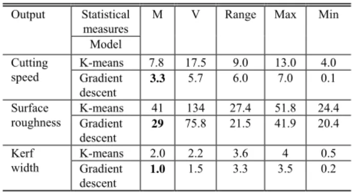
The models were validated against the experimental results. The detailed statistical analysis for the prediction error for cutting speed, surface roughness and kerf width was given in Table IV. From the table, it is clear that except surface roughness, the absolute prediction error for cutting speed and kerf width were within the acceptable limit. RBFN with gradient descent technique yields better result than with k-means technique.

TABLEIV MODEL VALIDATION RESULTS

IV. OPTIMIZATION BY NEURO-GENETIC TECHNIQUE

Although three output parameters were considered in the present study, multi-objective optimization was done only on two parameters. They are cutting speed and kerf width. The objective of a process engineer is to maximize the

cutting speed and minimize the kerf width simultaneously. These two objectives are conflicting in nature as already discussed in section I. Therefore, this problem is a multi-objectives optimization problem. In case of multi-objective optimization problem, a single solution which is the best with respect to all the objectives may not exist. The solutions for such situation are known as Pareto-optimal solutions or non-dominated solutions. Since NSGA-II works with a population of points, a number of Pareto-optimal solutions may be obtained using this technique. In the present work, RBFN based NSGA-II (Neuro-Genetic technique) was used to obtain Pareto-optimal solutions. The next sections will provide a brief idea of the NSGA-II algorithm [26] and optimization results.

A. Development of RBFN based NSGA-II

The goals of the NSGA-II algorithm are to find a set of solutions as close as possible to the Pareto-optimal front and simultaneously as diverse as possible. Except for the fitness assignment method, the basic structure of NSGA-II is similar to that of GA. The steps involved in this algorithm are briefly explained.

Step 1: Random binary population initialization: A binary population P of size N is generated randomly. A population consists of a set of input process parameters and is also used in making a solution which will produce outputs from the input-output relationship. The binary coded parameters are then converted into real value by a linear mapping, considering their upper and lower limits. The binary string of each parameter is converted into real value by the following expression:







2 1



U L

x_i x_i

L D

x_i x_i x_i

lsi 

  

 (11)

where,

_xi

is the real value of the ith input parameter, _xiL and _xiUare the lower and upper limits of the ith input parameters, respectively; _lsi is the string length of the ith

input parameter, and _xiD is the decoded value of the ith

parameter. Before feeding these real values to RBFN model, these raw values are required to be normalized. After normalizing these real values in the range 0.1 to 0.9, the fitnesses of the objective functions are obtained by the best RBFN model. Here RBFN network makes the hidden relationship between input and output variables, and thus formulates the objective functions.

Step 2: Fast non-dominated sorting: The population is sorted based on their non domination levels. The detailed explanation of this technique is described else-where [12]. In this technique two entities are calculated, first one is the domination count (ni) that represents the number of solutions which dominate the solution i and the second one isSithat represents the number of solutions which are dominated by the solutioni. This is accomplished by comparing each solution with every other solution and checked whether the solution under consideration satisfies the rules given below.

Output Statistical measures

M V Range Max Min

Model Cutting

speed

K-means 7.8 17.5 9.0 13.0 4.0

Gradient descent

3.3 5.7 6.0 7.0 0.1

Surface roughness

K-means 41 134 27.4 51.8 24.4

Gradient descent

29 75.8 21.5 41.9 20.4

Kerf width

K-means 2.0 2.2 3.6 4 0.5 Gradient

descent

1.0 1.5 3.3 3.5 0.2

Objective1_i Objective1_j and Objective2_i Objective2 or_j

Objective1_i Objective1_j and Objective2_i Objective2_j

 

  (12)

where, Objective1i and Objective1j are the fitness of objective1 for the ith and jth solution, respectively. Similarly, _Objective2i and _{Objective2 j} are the fitness of objective2 for the ith and jth solution, respectively. If the rules are satisfied, then the solution j is dominated else non-dominated. Thus the whole population is divided into different ranks. Ranks are defined as the several fronts generated from the fast non-dominated sorting technique such that Rank1 solutions are better than the Rank2 solutions and so on. This technique drastically reduces the computational time.

Step 3: Crowding distance: Once the populations are sorted, crowding distance is assigned to each individual belonging to each rank. This is because the individuals of the next generation are selected based on the rank and the crowding distance. This crowding distance ensures a better spread among the solutions. A better spread means a better diversity among the solutions. In order to calculate crowding distance, fitness of the objective functions for the solutions belonging to a particular rank were sorted in descending order with respect to each objective. An infinite distance is assigned to the boundary solutions i.e., for the first and nth solution, if n number of solutions belong to a particular rank. This ensures that the individuals in the boundary will always be selected and hence, result in better spread among the solutions. For other solutions belonging to that rank, the crowding distances are initially assigned to zero. For r2to n1solutions, this is calculated by the following formula:

( 1) ( 1)

( ) ( )

max min

f_m r f_m r I r m I r m

f_m f_m

  

 

 (13)

where, I r m( ) is the crowding distance of the of the rth individual for mthobjective, where,

m

=1 to 2. f_m(r1) is the value of the mthobjective for (r1)th individual,

max

fm and fmmin are the maximum and minimum values of the mthobjective, respectively.

Step 4: Crowded tournament selection: A crowded comparison operator compares two solutions and returns the winner of the tournament. A solution i wins a tournament with another solution j if any of the following conditions are true: (i) If solution i has a better rank than j (ii)If they have the same rank but solution i has larger crowding distance than solution j.

Step 5: Recombination and selection: The offspring and current population are combined and selection is done in order to obtain the population of the next generation. The offspring are generated by 2-point cross over and bitwise mutation. The elitism is ensured, as the best population from the offspring and parent solutions are selected for the next generation. The 2N solutions are then sorted based on their non-domination; and crowding distances are calculated for

all the individuals belonging to a rank. In order to form the population of the current generation, the individuals are taken from the fronts subsequently unless it reaches to the desired population number (N). The filling starts with the best non-dominated front (Rank1 solutions), with the solutions of the second non-dominated front, followed by the third non-dominated front, and so on. If by adding all individuals in a front the population exceeds N, then individuals are selected based on their crowding distance. The steps are repeated until maximum generation number is reached.

B. Optimization Results

The objective of the present study is to maximize the cutting speed and minimize the kerf width. In order to convert the second objective into maximization, it is suitably modified. The objectives then take the following form:

1

Objective 1 Cutting speed

Objective 2

Kerf width 

 (14)

As the range and the step length of the process variables were different, hence, different bit size was assigned to individual parameters. Initially bit lengths for individual parameters were taken arbitrarily. Finally optimal bit lengths were obtained by trial and error method. The optimal bit lengths for WF , Ton, Toff, IP , C and Vgap were found to be5,

10, 15, 5, 5, and 15, respectively. And hence, the string length of each chromosome (population) became 55. NSGA-II starts with 100 initial populations (N) which were generated randomly. Any other value of N could also be considered. Here a solution indicates a set of combination of input process parameters. Each set of parameters is producing a cutting speed and kerf width data through RBFN model.

Fig.2. Solutions are making four frontiers after thirteen generation.

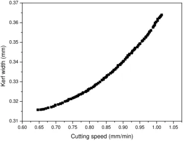
After finding the frontiers, the crowding distance was calculated for each individual by applying equation 13. The Crowding distance selection operator helps NSGA-II in distributing the solution uniformly to the frontier rather than bunching up at several good points. This was done by maintaining diversity in the population. The diversity in the population gives a wide range of choices to the users. Subsequently, the solutions of four frontiers were converged into only single front at the end of 250 generations. This was achieved by applying NSGA-II (step 1 to step 5) on those 100 initial solutions. Hence, at the end of 250 generations the scattered initial solutions are lying in the Pareto front leading to the final set of solutions. This is shown in Fig. 3. Thisgraph indicates that the Pareto front contains 100 non-dominated solutions. So far as the NSGA-II parameters were concerned, 2-point cross over with cross over probability 0.9 and bitwise mutation with mutation probability 0.1 were used. The tuning of these parameters was done by trial and error method.

Fig.3. Pareto-optimal solutions after 250 generation

The Pareto-optimal solutions using NSGA-II with RBFN technique is listed in Table V. In this table, out of hundred data, only first fifteen are presented.

TABLEV PARETO-OPTIMAL SOLUTIONS

As none of the solutions in the Pareto front are better than other, any one of them is an acceptable solution. The choice of one solution over other exclusively depends upon the requirement of the process engineers. If a higher cutting speed or a lower kerf width is required, a suitable combination of process variables could be selected from Table V. It could be shown that by using the non-dominated sorting genetic algorithm, the performance of the WEDM process could significantly be improved by selecting proper input process parameters. For an instance, it could be observed from the experimental results as tabulated in Table V, that the parametric combination for experiment number 12 produces cutting speed values of 0.615 mm/min and kerf width of 0.329 mm. By optimizing using RBFN based NSGA-II, the cutting speed could be increased by 34.9 % for the same kerf width (Sl. no. 11). This has been achieved by selecting proper input condition of the process.

V. CONCLUSION

The proposed Neuro-Genetic technique will be useful in finding several optimum solutions in multi-objective optimization problem. Here only two objectives were considered. In future, Pareto solutions can be obtained by considering three objectives simultaneously.

REFERENCES

[1] R.A. Mahdavinejad and A. Mahdavinejad, “ED machining of WC-Co,” Journal of Material Processing Technology, vol. 162-163, pp. 637-643, 2005.

[2] K. P. Rajurkar and W. M. Wang, “Thermal modeling and on-line monitoring of wire-EDM,” Journal of Material Processing Technology, vol. 38, pp. 417-430, 1993.

[3] S. Saha, M. Pachon, A. Ghoshal and M. J. Schulz, “Finite element modeling and optimization to prevent wire breakage in electro-discharge machining,” Mechanics Research Communications, vol. 31, pp. 451-463, 2004.

[4] P. Saha, A. Singha, S.K. Pal and P. Saha, “Soft computing models based prediction of cutting speed and surface roughness in wire electro-discharge machining of tungsten carbide cobalt composite,” International Journal of Advanced Manufacturing Technology, vol. 39, pp.74-84, 2008.

[5] Y.S. Trang, S.C. Ma and L.K. Chung, “Determination of optimal cutting parameters in wire electrical discharge machining,” International Journal of Machine Tools and Manufacturing, vol. 35, pp. 1693-1701, 1995.

[6] S. Sarkar, S. Mitra and B. Bhattacharyya, “Parametric optimization of wire electrical discharge machining of  titanium aluminide alloy through an artificial neural network model,” International Journal of Advanced Manufacturing Technology, vol. 27, pp. 501-508, 2006. [7] T.A. Spedding and Z.Q. Wang, “Parametric optimization and surface

characterization of wire electrical discharge machining process,” Precision Engineering, vol. 20, pp. 5-15, 1997.

[8] D. Scott, S. Boyina and K.P. Rajurkar, “Analysis and optimization of parameter combination in wire electrical discharge machining,” International Journal of Production Research, vol. 29, pp. 2189-2207, 1991.

[9] S. Chen and B. M. Mulgrew, “Adaptive Bayesian feedback equalizer based on a radial basis function networks,” IEEE International Conference on Communications, Chicago, vol. 3, pp. 1267-1271, 1992.

[10] J.S.R Jang, C.T Sun and E. Mizutani, “Neuro-Fuzzy and Soft Computing,” Prentice Hall of India Private Limited, New Delhi, 2005. [11] M. Taghi, V. Baghmisheh and N. Pavesic, “Training RBF networks

with selective backpropagation,” Neurocomputing, vol. 62, pp. 39-64, 2004.

[12] K. Deb, A. Pratap, S. Agarwal and T. A. Meyarivan, “Fast and elitist multiobjective genetic algorithm: NSGA-II.” IEEE Transactions, Evolutionary Computation, vol. 6, no. 2, pp. 182-197, 2002. Sl

No.

Input process parameters CS KW

WF Ton Toff Ip C Vgap

1 6 16 20 4 2.0 57 1.03 0.364 2 6 15 31 3 0.5 56 0.65 0.316 3 6 17 20 4 0.7 56 0.98 0.356 4 6 17 20 4 0.8 56 0.99 0.358 5 6 15 20 2 0.5 56 0.83 0.330 6 6 15 27 2 0.5 56 0.68 0.317 7 6 16 28 2 0.5 56 0.69 0.317 8 6 17 20 3 0.5 56 0.91 0.341 9 6 17 26 2 0.5 56 0.71 0.319 10 6 16 20 2 0.5 56 0.84 0.331 11 6 17 20 2 0.5 56 0.83 0.329 12 6 17 20 4 0.5 56 0.94 0.348 13 6 17 20 3 0.5 56 0.86 0.334 14 6 16 20 4 0.5 56 0.96 0.351 15 6 17 20 3 0.5 56 0.86 0.334 CS = cutting speed, KW = Kerf width

0.60 0.65 0.70 0.75 0.80 0.85 0.90 0.95 1.00 1.05 0.31

0.32 0.33 0.34 0.35 0.36 0.37

Ke

rf

width

(mm

)