ISSN : 2248-9622, Vol. 6, Issue 7, ( Part -3) July 2016, pp.89-96
Intermodulation Distortion Cancellation by Feedforward
Linearization of Power Amplifier
Amanpreet Kaur*, Rajbir Kaur**
*Department of Electronics and Communication Engineering, Punjabi University, Patiala, India ** Department of Electronics and Communication Engineering, Punjabi University, Patiala, India
ABSTRACT
Intermodulation distortion has been a major source of linearity when a power amplifier is used for multichannel systems in wireless communication. Since, distortion products appear close to original input carriers they need to be cancelled out so that information reaches unaltered and distortion-less at the destination. In this paper, feedforward technique has been selected to obtain maximum intermodulation distortion reduction. To demonstrate linearity improvement, along with IMD measurement, carrier to IMD power ratio (C/I) and intercept points are also evaluated. Later on, the feedforward power amplifier is tested by sweeping input power within a specified range and graphs for IMD and intercept points are derived. The results show that the feedforward linearized power amplifier achieves best results when operated at input power levels around and above -12 dBm.
Keywords
:
Carrier to IMD power ratio (C/I), Feedforward (FF), Intercept point (IP), Intermodulation distortion (IMD), Linearization, Nonlinearity, Power amplifier (PA).I.
INTRODUCTION
The biggest milestone in the path of power
amplifier’s linearity is the intermodulation distortion
which is generated in power amplifier’s output when a multi-carrier signal is applied as an input. Alongside gain compression, harmonic distortion and adjacent channel interference [1]; it is very important to keep a check on the intermodulation distortion levels also to ensure a distortion-less and linear output. The intermodulation distortion products are basically the additional tones generated from multi-carrier amplification appearing in the vicinity of the original transmitted carriers [2]. These extra undesired frequencies may pose a threat of adjacent channel interference [3]. Intermodulation distortion of third-order, fifth-order or seventh-order is generally characterized by their corresponding intercept point (IP) [4]. Since, third-order intermodulation distortion appears closest to the original carriers; the third-order intercept point is of much greater concern. The greater the third-order intercept point better is the linearity and lower is the third-order intermodulation distortion [5].
The linearization process aims to modify the amplifier output in such a way that only linearized and undistorted signal is achieved at the final output of linearization stage. Several linearization methods are available today to provide the necessary distortion cancellation. The most popular include predistortion, feedforward and feedback [6]. Feedforward technique having decent potential of managing the multi-carrier signal [7], presenting wide bandwidth and good cancellation of IMD [8] is preferred.
Feedforward works on the principle of
suppressing the amplifier’s output to input level, subtracting the resulting signal from input itself giving only distortion, then amplifying the distortion and finally subtracting the amplified distortion from amplified input resulting in linearized output [9]. The traditional feedforward topology was used to linearize a third-generation PA in [10] but due to 180º phase difference of upper and lower distortion products the upper and lower IMD levels were unevenly cancelled. Whereas in [7] using the common feedforward method and proper setting of delays in both loops, somewhat close and even IMD cancellation was achieved. In [11] an improved over-compensation FF method was presented and in [12] the feedforward technique was upgraded with another distortion cancellation loop to provide further improved linearity. But these two improved circuits are rather much more complex and increase the cost of
implementation for a small additional IMD
cancellation where much more IMD reduction can be achieved by proper setting of amplitude and phase shifters along with careful selection of error amplifier. In this paper, the vintage feedforward topology is implemented to linearize a 16W WCDMA power amplifier [13] used for repeater applications in frequency range of 2110-2170 MHz. To demonstrate the effectiveness of this approach intermodulation distortion levels are measured upto seventh order and compared with those from a non-linearized PA. The distance between original carriers and IMD products is measured and the intercept points (IP) are computed. The paper is organized as follows: section
II describes how the intermodulation distortion is generated by taking a multicarrier signal as an example, section III describes the basic working of feedforward technique, section IV describes the simulation and results and section V gives the conclusion.
II.
INTERMODULATION
DISTORTION
A power amplifier when subjected to a two-tone signal generates intermodulation products in the output resulting in nonlinearity. It must be noted that not all the harmonics in the output of amplifier are problematic. Let us see how these harmonics are
generated at the amplifier’s output.
Let Vin be the signal given as input to power
amplifier. Then the output of amplifier expressed by expanding the power series [14] will be:
Vout = A1Vin+ A2 Vin 2+ A3 Vin 3+⋯+
An Vin n (1)
Let input signal consists of two carriers of dissimilar frequencies, i.e., the signal is a two tone signal given by,
Vin = k cosω1t + k cosω2t (2)
where, ω1≠ω2. The first term of (1) gives fundamental
tones at the frequencies of ω1and ω2 as shown below:
A1Vin = A1 k cosω1t + k cosω2t (3)
The second term of output in (1) can be expanded mathematically as,
A2 Vin 2= A
2 k cosω1t + k cosω2t 2 = A2 k2cos2ω1t + 2k2cosω1t. cosω2t +
k2cos2ω2t (4) The first and last term of (4) are straightforward and gives harmonics at the frequencies of 2ω1 and 2ω2. But the second term is rather complex and needs to be simplified as shown below:
2k2cosω
1t. cosω2t = k2. 2 cosω1t. cosω2t (5)
Using trigonometric identity: 2 cos A . cos B = cosA+B+ cosA−B in (5) we get,
2k2cosω
1t. cosω2t = k2 cos ω1+ω2 t + cosω1−ω2t
= k2cos ω
1+ω2 t + k2cos ω1−ω2 t (6)
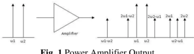
So, as seen in (6), we get two second-order products at the frequencies of (ω1 + ω2) and (ω1 – ω2) respectively. These signals do not pose much problem because they merely come outside the amplifier bandwidth as shown in Fig. 1.
Fig. 1 Power Amplifier Output
Now, the third term of amplifier output is given by,
A3 Vin 3= A
3k cosω1t + k cosω2t 3 = A3k3cos3ω1t + 3k3cos2ω1t. cosω2t + 3k3cosω
1t. cos2ω2t + k3cos3ω2t (7)
Here also, the first and last term are the harmonics at the frequencies of 3ω1and 3ω2. Whereas, the second and third terms need to be solved mathematically as shown below:
3k3cos2ω
1t. cosω2t = 3k3cosω2t cos2ω1t (8)
Using trigonometric formulae: cos2A = 1+cos 2A 2 & 2 cos A . cos B = cos A + B + cos A−B in (8) we get,
3k3cos2ω1t. cosω2t = 3 k3cosω2t
1+cos 2ω1t
2
= 3 2k
3cosω 2t +
3 2k
3cosω
2t . cos 2ω1t
= 3 2k
3cosω 2t +
3 4k
3 2 cos 2ω
1t . cosω2t
= 3 2k
3cosω 2t +
3 4k
3 cos 2ω
1+ ω2 t + cos2ω1−ω2t (9) Similarly,
3k3cosω
1t. cos2ω2t = 3
2k 3cosω
1t + 3 4k
3 cos 2ω
2+ ω1 t +
cos2ω2−ω1t (10) Therefore, as observed from (9) and (10), the second and third terms of (7) result in four additional signals at the frequencies of (2ω1 + ω2), (2ω2+ ω1), (2ω1 –
ω2) and (2ω2 – ω1). Out of these signals, the most
problematic are (2ω1 – ω2) and (2ω2 – ω1) and the signals at these frequencies are known as third-order intermodulation products. Observing these second-order and third-second-order frequency terms, it is evident that higher order terms will be sum or difference of
integer multiples of ω1 & ω2. So, in general all possible distortion terms in output of amplifier can be calculated by using the term αω1±βω2, where α & β are integers. Therefore, fifth-order intermodulation products will appear at the frequencies of (3ω1–2ω2)
& (3ω2 – 2ω1) and seventh-order intermodulation
products will be present at the frequencies of (4ω1 – 3ω2) & (4ω2 – 3ω1). These intermodulation products are a major concern and need to be removed to ensure linearity. The Table 1 below shows the different IMD products.
Table 1 Intermodulation products
Order Intermodulation Products Low Side High Side
3 2ω1–ω2 2ω2–ω1
5 3ω1–2ω2 3ω2–2ω1
7 4ω1–3ω2 4ω2–3ω1
III.
FEEDFORWARD
LINEARIZATION
ISSN : 2248-9622, Vol. 6, Issue 7, ( Part -3) July 2016, pp.89-96
feedforward linearization. The motivation behind this invention came while he was working to minimize distortion in multiplex telephone systems where
multiple amplifiers’ distortion may sum together and
degrade the output audio signal [16].
Fig. 2 Feedforward technique
The block diagram of feedforward linearization method is shown in Fig. 2 [9]. There are two loops; first loop is signal cancellation loop and second is error cancellation loop. The input signal Pin in the first
loop is amplified by main power amplifier giving PMA.
The amplifier output consists of amplified input signal and intermodulation distortion products generated due
to amplifier’s non-linearity i.e.,
PMA = APin+ DIM (11)
where, A is gain of main power amplifier and DIM is
the intermodulation distortion.
Fixed attenuator with attenuation factor A0 then brings
down this amplified signal, making it equal to input signal itself plus the distortion.
P0= PMA A0 =
APin A0 +
DIM
A0 (12)
Since, the value of fixed attenuator is chosen to match the gain of main power amplifier [8], so A0= A.
Therefore, changing the denominator of first term of (12) we get,
P0= APin
A + DIM
A0 P0= Pin+ DIM
A0 (13)
This signal in (13) is then combined with attenuated, phase adjusted and delayed lower branch signal giving the error signal Pe consisting of only distortion.
Pe= Pi+ P0 (14) where, Pi= Pinθ1 and θ1 is the phase shift introduced
by phase shifter. Therefore, (14) becomes,
Pe= Pi+ Pin+ DIM
A0 (15)
Now, we know that input is delayed in phase, so we have Pi= −Pin or Pi= Pin+ 180° and therefore the
error signal becomes,
Pe= −Pin + Pin+ DIM
A0 Pe=
DIM
A0 (16)
The error signal is then phase shifted giving
Pe1= Peθ2 and amplified by error amplifier by an
equal amount with which the main amplifier output was attenuated giving amplified error signal,
PEA = A0Pe1= A0Peθ2= A0 DIM
A0 θ2= DIMθ2 (17)
And then this signal is combined with delayed amplifier output signal, thereby finally giving linearized, distortion-less signal at the output.
Pout = PMA+ PEA (18)
Pout = APin+ DIM+ DIMθ2
Pout = APin (∵DIMθ2=−DIM) The amplitude and phase shifters having broadband tunable characteristics are the main components that make the necessary adjustments so as to obtain minimum intermodulation distortion levels [17].
IV.
SIMULATION
AND
RESULTS
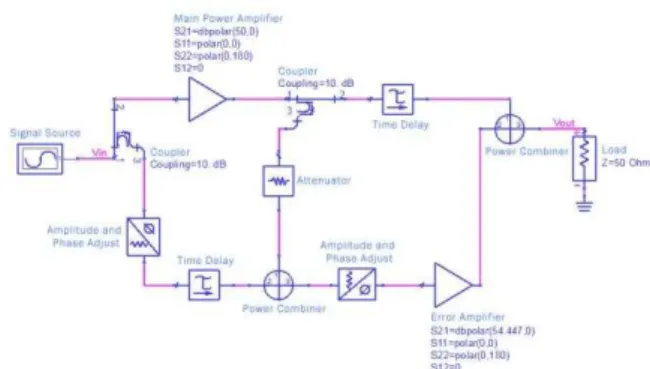
The implementation of simulation circuit for
feedforward linearization of 16W WCDMA
multicarrier power amplifier [13] is shown in Fig. 3.
Fig. 3 Feedforward linearization circuit
4.1 Measurement of Intermodulation Distortion and Carrier to IMD power ratio (C/I)
For the measurement of amount of IMD cancellation, we used two-tone test. The simulation circuit for two-tone analysis is shown in Fig. 4. The fundamental frequency of the input signal is taken as RFfreq = 2125 MHz, the spacing between carriers is chosen as fc = 10 MHz. Therefore, the frequencies of
two tones (f1 and f2) and the third-order, fifth-order
and seventh-order IMD products are calculated as, Input carriers:
f1= RFfreq− fc
2 = 2125− 20
2 = 2120 MHz f1= RFfreq +
fc
2 = 2125 + 20
2 = 2130 MHz
3rd-order IMD:
2f1−f2= 22120 −2130 = 2110 MHz
2f2−f1= 22130 −2120 = 2140 MHz
5th-order IMD:
7th-order IMD:
4f1−3f2= 4 2120 −3 2130 = 2090 MHz
4f2−3f1= 4 2130 −3 2120 = 2160 MHz
Firstly, the simulation is carried out at the input power level of -8 dBm near the saturation and 1dB compression point to calculate the new IMD levels and then the input power is varied to analyze how the intermodulation distortions are affected as the input power is changed.
Fig. 4 Two-tone analysis setup
Before applying any linearity circuit, the output of the amplifier is obtained as shown in Fig. 5.
Fig. 5 IMD in amplifier output before linearization
The output of amplifier after applying linearity method is shown in Fig. 6.
Fig. 6 Reduced IMD in amplifier output after linearization
Therefore, from Fig. 5 & Fig. 6, we examine a great decrease in the amount of intermodulation distortion. Comparison between IMD values before and after linearization is given in Table 2 and Table 3 gives the comparison of C/I i.e. distance between intermodulation distortion and carrier signal values.
Table 2 IMD before and after linearization
Order
Intermodulation distortion (dBm) Before
linearization
After linearization Low
side
High side
Low side
High side
3 22.443 22.444 -76.240 -76.240
5 8.849 8.845 -86.819 -86.817
7 -12.237 -12.170 -104.307 -104.274
Table 3 C/I before and after linearization
Order
C/I (dB) Before
linearization
After linearization Low
side
High side
Low side
High side
3 14.605 14.605 112.236 112.237
5 28.200 28.203 122.816 122.814
7 49.285 49.218 140.304 140.271
4.2 Intermodulation Distortion with swept power
To determine how intermodulation distortion alters as we sweep the input power of both the carriers, we apply a sweep of RF power within the range of -20 dBm to 20 dBm and make a comparison for non-linearized and linearized amplifier through graphs. Fig. 7, Fig. 8 and Fig. 9 give the comparison of 3rd-order, 5th-order and 7th-order IMD variations with input power.
Fig. 7 Variation of 3rd-order IMD with input power
ISSN : 2248-9622, Vol. 6, Issue 7, ( Part -3) July 2016, pp.89-96
Fig. 8 Variation of 5th-order IMD with input power
Fig. 8 shows that 5th-order IMD which was -49.800 dBm at lowest input power of -20 dBm on both low and high side before linearization has now reduced to -123.895 dBm after linearization. At input power between -13 dBm & -10 dBm, it almost remains constant at -100 dBm approximately and after -10 dBm it increases with increase in input power but always remains at lower levels as compared to the non-linearized case.
Fig. 9 Variation of 7th-order IMD with input power
In Fig. 9, it is noticed that 7th-order IMD was lowest before linearization upto -12 dBm of power input. But after that it increases gigantically at input power level of -11 dBm from -304.221 dBm at -12 dBm to -85.453 dBm at -11 dBm and increases afterwards. Whereas, after linearization it is higher below input power of -12 dBm and becomes lower after that as compared to the case when no linearity method was applied and remains less up to 20 dBm power input. Therefore, 7th-order IMD decrease is spotted after power level of -12 dBm. The Table 4 below gives IMD values for different input powers.
Table 4 IMD values at different input powers for FF amplifier
IMD (dBm)
Input Power (dBm)
-20 -10 0 10 20
IMD3- -99.518 -78.651 -38.287 -2.206 28.842
IMD3+ -99.518 -78.651 -38.287 -2.206 28.842
IMD5- -123.895 -100.250 -52.848 -30.684 -36.373
IMD5+ -123.895 -100.250 -52.854 -30.719 -36.339
IMD7- -151.093 -104.565 -70.109 -33.606 -10.804
IMD7+ -151.093 -104.565 -70.149 -33.965 -12.095
4.3 Measuring the Input and Output Intercept Points
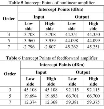
The input and output intercept points play a very crucial role as linearity determinant. Higher intercept points are always preferred. So, we used the similar two-tone analysis method previously applied to determine IMD suppression. The simulation gave the values of input and output intercept points up to seventh order. Table 5 and Table 6 give the calculated values at input power of -8 dBm.
Table 5 Intercept Points of nonlinear amplifier
Order
Intercept Points (dBm)
Input Output
Low side
High side
Low side
High side
3 -3.708 -3.708 44.351 44.350
5 -3.960 -3.959 44.098 44.099
7 -2.796 -2.807 45.262 45.251
Table 6 Intercept Points of feedforward amplifier
Order
Intercept Points (dBm)
Input Output
Low side
High side
Low side
High side
3 45.108 45.108 92.115 92.115
5 19.694 19.693 66.701 66.700
7 12.374 12.368 59.381 59.375
4.4 Intercept points with swept power
Fig. 10 Input TOI
The graph shows an increase in input third-order intercept point for feedforward amplifier. At -20 dBm of input power it is 38.747 dBm as compared to -4.628 dBm of nonlinear amplifier. It is hiked at input power of -6 dBm with a value of 53.203 dBm on lower side and 53.199 dBm on higher side.
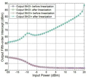
Fig. 11 Input 5thOI
In 5thOI graph, it is clearly seen that feedforward amplifier has much higher values of 5thOI than nonlinear amplifier. At input power of -20 dBm, it has increased from -3.154 dBm for nonlinear amplifier to 13.963 dBm for FF amplifier. It experiences a bump at -10 dBm of input power with a value of 20.551 dBm on lower side and 20.552 dBm on higher side and then it further increases with increase in input power. One must notice here that the values of input 5th-order intercepts obtained after linearization are always greater than the values measured before linearization. That is why the graph is increasing upwards and is always higher than the case with no linearization applied.
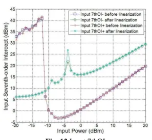
Fig. 12 Input 7thOI
The above graph shows that input seventh-order intercept after linearization is firstly less up to -12 dBm, after that it increases as compared to the case when no linearization was applied. It experiences a sudden increase at -4 dBm input power and remains high for linearized case afterwards. Therefore, from all the graphs for input intercept points we conclude that input TOI and 5thOI are always higher for feedforward amplifier whereas input 7thOI only increases after -12 dBm of input power. Now, we will see how output intercept points behave as we vary RF power input. Fig. 13, Fig. 14 and Fig. 15 show the output intercept points of third-order, fifth-order and seventh-order respectively.
Fig. 13 Output TOI
ISSN : 2248-9622, Vol. 6, Issue 7, ( Part -3) July 2016, pp.89-96
Fig. 14 Output 5thOI
The above graph gives output fifth-order intercept point before and after linearization at different power levels. While 5thOI for nonlinear amplifier is decreasing as input power is increased, 5thOI for FF amplifier increases with input power.
Fig. 15 Output 7thOI
In Fig. 15, we see that up to input power of -12 dBm, the output seventh-order intercepts for feedforward amplifier are lower than nonlinear amplifier but after that it increases. Also, it experiences a sudden increase at -4 dBm input power with values 68.755 dBm on lower side and 73.855 dBm on higher side. Therefore, we here deduce that like input intercept points, output 3rd-order and 5th -order intercept points are also higher for feedforward amplifier but output 7th-order intercept point increase only after -12 dBm of input power. Hence, we can say that input intercept points and output intercept points
of all orders behave somewhat alike after
linearization. The Table 7 below gives input and output intercept point’s values for different input powers.
Table 7 Intercept Points for FF amplifier at different input powers
Intercept Point (dBm)
Input Power (dBm)
-20 -10 0 10 20
Input
TOI- 38.747 43.313 38.131 35.074 34.340
TOI+ 38.747 43.313 38.131 35.073 34.340
5thOI- 13.963 20.551 21.201 28.151 41.969
5thOI+ 13.963 20.552 21.202 28.160 41.960
7thOI- 6.171 10.083 16.007 21.584 29.381
7thOI+ 6.171 10.083 16.014 21.644 29.596
Output
TOI- 85.754 90.321 85.137 82.045 80.893
TOI+ 85.754 90.321 85.137 82.045 80.893
5thOI- 60.970 67.559 68.206 75.123 88.522
5thOI+ 60.970 67.559 68.208 75.132 88.513
7thOI- 53.178 57.091 63.013 68.556 75.934
7thOI+ 53.178 57.090 63.020 68.616 76.149
Therefore, by feedforward analysis we have been able to decrease distortion and increase linearity of amplifier.
V.
CONCLUSION
47.764 dBm, 22.603 dBm, 14.119 dBm on lower side and on higher side of fundamental carriers the increment is 47.765 dBm, 22.601 dBm, 14.124 dBm for output 3rd-order, 5th-order, 7th-order intercepts respectively. Moreover, by varying RF input power it is observed that both IMD and intercept points are always better after -12 dBm of input power. Therefore, the feedforward linearized power amplifier will give best results in terms of IMD cancellation and intercept point increase when operated around and above power levels of -12 dBm.
REFERENCES
[1] A.S. Mahmoud, H.N. Ahmed, “A novel
nonlinearity measure for RF amplifiers in
jamming applications,” 33rd National Radio Science Conference (NRSC), Aswan, 2016, 398-405.
[2] A. Katz, “Linearizing High Power Amplifiers,” in Linearizer Technology, 1-19.
[3] E.A. Hussein, M.A. Abdulkadhim,
“Performance Improvement of BER in OFDM
System using Feed Forward Technique on
Power Amplifier,” International Journal of Computer Applications, 75(4), 2013, 35-39. [4] B.R. Jackson, C.E. Saavedra, “A CMOS
Amplifier with Third-Order Intermodulation
Distortion Cancellation,” IEEE Topical Meeting on Silicon Monolithic Integrated
Circuits in RF Systems, SiRF ’09., San Diego,
CA, 2009, 1-4.
[5] L. Frenzel, “What’s The Difference Between The Third-Order Intercept And The 1-dB Compression Points?,” in ElectronicDesign, 2013. [Online]. Available: http://electronicdesig n.com/what-s-difference-between/what-s- difference-between-third-order-intercept-and-1-db-compression-point. Accessed: Jul. 14, 2016. [6] A. Katz, J. Wood and D. Chokola, “The Evolution of PA Linearization: From Classic Feedforward and Feedback Through Analog
and Digital Predistortion,” in IEEE Microwave Magazine, 17(2), 2016, 32-40.
[7] M.K. Ibrahim, “Feedforward Linearization of a Power Amplifier for Wireless Communication
Systems,” Journal of Babylon University, Engineering Sciences, 21(4), 2013, 1183-1193. [8] S.P. Stapleton, “Presentation on Adaptive
Feedforward Linearization of RF Power Amplifiers - Part 2,” Agilent EEsof EDA, 2001.
[9] Agilent Technologies - Advanced Design
System 2011.01, “Linearization DesignGuide,”
2011.
[10] M.H.C.S. Muñiz, A.V. Ventura, “Feedforward linearization of a power amplifier for wireless
communication systems,” in International Meeting of Electrical Engineering Research, 2006, 164-168.
[11] H. Ma, Q. Feng, “An Improved Design of
Feed-forward Power Amplifier,” PIERS
Online, 3(4), 2007, 363-367.
[12] M.A. Honarvar, M.N. Moghaddasi and A.R.
Eskandari, “Power Amplifier Linearization
Using Feedforward Technique for Wide Band
Communication System,” Radio-Frequency Integration Technology, IEEE International Symposium. RFIT 2009, 72-75.
[13] “PCM5A5ECO (SJU 7084) datasheet,” Solid
State Personal Communication Power
Amplifier, Empower RF Systems.
[14] Z. El-Khatib, L. MacEachern and S.A.
Mahmoud, “Modulation Schemes Effect on RF
Power Amplifier Nonlinearity and RFPA
Linearization Techniques,” Distributed CMOS Bidirectional Amplifiers: Broadbanding and Linearization Techniques,Analog Circuits and Signal Processing, Springer Science & Business Media, 2012, 7-28. [Online]. Available: http://www.springer.com/cda/conten t/document/cda_downloaddocument/97814614 02718-c1.pdf?SGWID=0-0-45-1329438-p174124973. Accessed: Jul. 15, 2016.
[15] H.S. Black, “Inventing the negative feedback
amplifier,” Spectrum, IEEE, 14(12), 1977, 55-60.
[16] A. Katz, D. Chokola, “The Evolution of
Linearizers for High Power Amplifiers,” in Microwave Symposium (IMS), 2015 IEEE MIT-S International, 2015, 1-4.
[17] H. Park, H. Yoo, S. Kahng and H. Kim,
“Broadband Tunable Third-Order IMD Cancellation Using Left-Handed Transmission-Line-Based Phase Shifter,” in IEEE Microwave
and Wireless Components Letters, 25(7), 2015, 478-480.
[18] R. Kaur, M.S. Patterh, “Analysis and Measurement of Two Tone intermodulation
distortion in Wideband Power Amplifier,” International Journal of Engineering Trends and Technology (IJETT), 29(4), 2015, 188-191. [19] R.N. Braithwaite, “Analog Linearization Techniques Suitable for RF Power Amplifiers