Common Distributions
Anton K. Formann*
Department of Psychological Basic Research, University of Vienna, Vienna, Austria
Abstract
An often reported, but nevertheless persistently striking observation, formalized as the Newcomb-Benford law (NBL), is that the frequencies with which the leading digits of numbers occur in a large variety of data are far away from being uniform. Most spectacular seems to be the fact that in many data the leading digit 1 occurs in nearly one third of all cases. Explanations for this uneven distribution of the leading digits were, among others, scale- and base-invariance. Little attention, however, found the interrelation between the distribution of the significant digits and the distribution of the observed variable. It is shown here by simulation that long right-tailed distributions of a random variable are compatible with the NBL, and that for distributions of the ratio of two random variables the fit generally improves. Distributions not putting most mass on small values of the random variable (e.g. symmetric distributions) fail to fit. Hence, the validity of the NBL needs the predominance of small values and, when thinking of real-world data, a majority of small entities. Analyses of data on stock prices, the areas and numbers of inhabitants of countries, and the starting page numbers of papers from a bibliography sustain this conclusion. In all, these findings may help to understand the mechanisms behind the NBL and the conditions needed for its validity. That this law is not only of scientific interestper se, but that, in addition, it has also substantial implications can be seen from those fields where it was suggested to be put into practice. These fields reach from the detection of irregularities in data (e.g. economic fraud) to optimizing the architecture of computers regarding number representation, storage, and round-off errors.
Citation: Formann AK (2010) The Newcomb-Benford Law in Its Relation to Some Common Distributions. PLoS ONE 5(5): e10541. doi:10.1371/ journal.pone.0010541
Editor:Richard James Morris, John Innes Centre, United Kingdom
ReceivedFebruary 3, 2010;AcceptedApril 8, 2010;PublishedMay 7, 2010
Copyright:ß2010 Anton K. Formann. This is an open-access article distributed under the terms of the Creative Commons Attribution License, which permits unrestricted use, distribution, and reproduction in any medium, provided the original author and source are credited.
Funding:The author has no support or funding to report.
Competing Interests:The author has declared that no competing interests exist.
* E-mail: anton.formann@univie.ac.at
Introduction
Newcomb [1] observed how much faster the first pages of tables of decadic logarithms wear out than the last ones, indicating that the first significant figure is oftener 1 than any other digit, and that the frequency diminishes up to 9. Without giving actual numerical data and a strict formal proof, he reached the conclusion that ‘‘The law of probability of the occurrence of numbers is such that all mantissae of their logarithms are equally probable’’, so that ‘‘every part of a table of anti-logarithms is entered with equal frequency’’. This resulted in a table giving the probabilities of occurrence in the case of the first two significant digits; see Table 1. More than a half century later, Benford [2] rediscovered Newcomb’s observation. Based on substantial empirical evidence from 20 different domains, such as the surface areas of 335 rivers, the sizes of 3259 U.S. populations, 104 physical constants, 1800 molecular weights, 5000 entries from a mathematical handbook, 308 numbers contained in an actual issue of Readers’ Digest, the street addresses of the first 342 persons listed in American Men of Science, and 418 death rates, Benford stated a logarithmic law of frequencies of significant digits. This law gives
p(a)~log(1za{1),a~1,. . .,9, ð1Þ
for the probabilityp(a)of the digitain the first place of observed numbers and
p(b)~X 9
a~1
log 1 z(10azb){1
,b~0,. . .,9, ð2Þ
for the probabilityp(b)of the second-place digitb. Most of the 20 domain-specific distributions of the first-place digits showed rather good agreement with the logarithmic law (1) – that later came to be known as Benford’s or Newcomb-Benford law (NBL) –, but the averaged distribution fitted nearly perfectly.
These findings initiated ‘‘a varied literature, among the authors of which are mathematicians, statisticians, economists, engineers, physicists, and amateurs’’, as Raimi [3] wrote in his comprehen-sive review on the first digit problem (p.521). After having described and discussed several approaches taken to ground the NBL, namely density and summability, scale-invariance, base-invariance, and mixture-distribution arguments, he concludes that – up to that time – Pinkham’s [4] scale-invariance argument gave the first theoretical explanation of the NBL, however assuming a cumulative distribution function that cannot exist [5], pp.253–264, and assuring only a miserable numerical approximation. As an example, on p.533 Raimi [3] mentions the half Cauchy distribution with scale parameter a and density f(x)~2a
p(x2za2)
first-place digit to be 1. But some 15 years earlier, Furry and Hurwitz [6] already had derived much more precise bounds for the half Cauchy distribution.
Since Raimi’s [3] review, the literature on the NBL has been expanded considerably. This can be seen from the bibliography compiled by Hu¨rlimann [7] in 2006 with its 350 entries and from the up-to-date online bibliography implemented by Berger and Hill [8] that actually lists nearly 600 sources related to the NBL. Major theoretical advances have to be attributed to Hill who showed in a series of papers that base-invariance implies the NBL [9,10], and that random samples coming from many random distributions may generate a compound distribution fulfilling the NBL [11]. Schatte [12] and Lolbert [13] studied the NBL in dependence on the numeral base, with the result that the approximation by the NBL becomes worse outside a limited range of bases. The relationship between the distribution of first digits with Zipf’s law, with prime numbers and Riemann zeta zeroes, and with order statistics was investigated by Irmay [14], Luque and Lacasa [15], and Miller and Nigrini [16], respectively. Further, it was shown that exponential random variables [17] and other survival distributions [18] obey the NBL, that mixtures of uniform distributions fulfill a (generalized) version of the NBL [19,20], and that data coming from different types of multiplica-tive processes also result in a first-digit distribution following the NBL [21–23] (but see also earlier results in [24,25]) as do geometric sequences, for example powers of two [3], p.525. Bounds for the approximation error to the NBL were given by Du¨mbgen and Leuenberger [26] for the (half-)normal, the log-normal, the Gumbel, and the Weibull (including the exponential) distributions.
The NBL has been shown to fit rather closely many empirical data: in addition to most of those analyzed by Benford [2], among others, stock index returns [27], stock prices [28], eBay auctions [29], and consumer prices half a year after the introduction of the Euro in 2002 [30]. In contrast, the latter study found deviations from the NBL due to psychological pricing (consumer prices preferably ending in 0, 5, or 9) immediately after and a full year after the introduction of the Euro. So, the NBL may be useful as a benchmark for detecting irregularities in data. This has become of widespread use in economic fraud detection (e.g. tax evasion) [31], but the NBL was also proposed as a means to identify possible problems with survey data [32], self-reported ratings [33], and scientific results [34]. Because of its prominence, the NBL found even entrance in esteemed newspapers [35]. Another, merely future field for putting the NBL into practice is computer design. Theoretical considerations concerned the interrelation between number representation and storage requirements, as well as round-off errors arising in the computation of products [10].
Interestingly, empirical evidence was provided by Torres et al. [23] that file sizes in PCs behave according to the NBL of the first and second digit. In all, the goal could be to optimize the architecture of computers in order to fasten precise calculations and to save storage, both by taking the implications of the NBL into account.
On the other hand, many data obey the NBL rather badly or simply not, for example some mathematical functions such as square roots and the inverse1=x. In his review, Raimi [3] gave two empirical examples for failure of the NBL: the 1974 Vancouver (Canada) telephone book, where no number began with the digit 1, and sizes of populations of all populated places with population at least 2500 from five US states according to the censuses from 1960 and 1970, where 19% only began with digit 1 but 20% with digit 2. To give but one recent empirical example, Beer’s [36] finding should be mentioned that terminal digits of data in pathology reports do not follow the NBL. A simple explanation of the incompatibility of empirical data with the NBL cannot be found in any case, but these three cases have their obvious peculiarities: assignment of telephone numbers in an arbitrary manner, truncation of population size at 2500 inhabi-tants, and rounding data, comparable to psychological pricing of consumer goods.
It seems that nowadays the practical potentialities of the NBL have been recognized, and that meanwhile this empirically derived law can be considered theoretically well-analyzed. However, its relation to common distributions of random variables was investigated up to now only rudimentary [6,17,18,26]. In addition, previous studies concentrated on the first digit, derived the deviation of the distribution under consideration from the NBL by calculating or approximating the respective integrals, and did not consider functions of random variables. In contrast, the present study investigates the leading ten digits and counts their frequencies from simulated data for different numbers of figures generated, whereby this is done not only for the random variables themselves, but also for ratios therefrom. This proceeding allows one to get an impression of the degree to which real data of finite sample size may approach the distribution predicted by the NBL while adopting one of Newcomb’s arguments stated in the second paragraph of his two-pages 1881 note [1]: ‘‘As natural numbers occur in nature, they are to be considered as the ratios of quantities. Therefore, instead of selecting a number at random, we must select two numbers at random, and inquire what is the probability that the first significant digit of their ratio is the digit n. To solve the problem we may form an indefinite number of such ratios, taken independently;… (p.39).
This statement suggests the interpretation that Newcomb did not intend to consider numbers stemming from one and the same domain, for example from one of those investigated later by Benford, but that he had in mind to consider numbers drawn at random from the universe of all possible domains. If so, the measurez(i)being available for an objectO(i)can be understood as the ratiox(i)=y(i)of the two numbersx(i)andy(i), wherex(i)
represents the object’s size ‘‘per se’’ andy(i)represents the scaling unit. In case that the objects stem from the same domain and were measured on the same scale, the scaling constant is no longer of interest and considering the measures z(i) as given entities is appropriate, the more so as the Newcomb-Benford distribution has been shown to be scale-invariant. (This means that performing an admissible transformation of the ratio scale – that is, by multiplying all of the values by a positive constant – does neither reduce nor improve the degree to which the NBL fits the data.) Therefore, both relations are of interest: within one domain the relation between the NBL and the distribution of a random Table 1.Probabilities of occurrence for first four digits
according to the Newcomb-Benford law.
Digit
Place 0 1 2 3 4 5 6 7 8 9
1. – 3010 1761 1249 0969 0792 0669 0580 0512 0458
2. 1197 1139 1088 1043 1003 0967 0934 0904 0876 0850
3. 1018 1014 1010 1006 1002 0998 0994 0990 0986 0983
4. 1002 1001 1001 1001 1000 1000 0999 0999 0999 0998
variable, and across domains the relation between the NBL and the ratio distribution of two random variables.
Methods
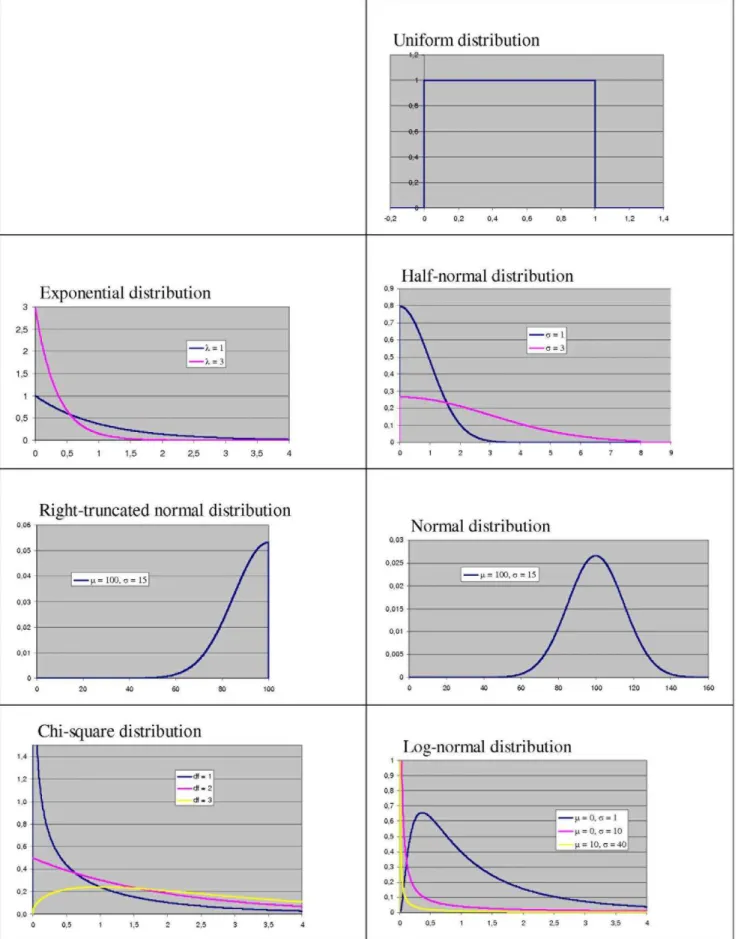
Out of the manifold of common distributions seven were selected for the simulation study. Criteria for inclusion were, first, that each one of the distributions gives support for x§0 only, second, that some of the earlier investigated distributions should be included in order to allow comparisons, and, third, that across the selected distributions their shape should vary from right-skewed to left-right-skewed, including symmetric distributions. The seven types of distributions illustrated in Figure 1 and the resulting ratio-distributions (cf. Figure 2 for some of them) are the following ones.
(a) Theuniform distribution,U½0,1, with density
f xð Þ~ 1 0 ƒxƒ1 0 otherwise,
ð3Þ
merely as a test for the pseudo-random number generator, and in the case of ratios Z~X=Y, with X and Y independent, because of the specific shape of the resulting density forf(z),
f zð Þ~
1=2 0vzv1
1
2z2
z§1 0 otherwise: 8 > < > : ð3aÞ
(b) Theexponential distribution,EXPð Þl, with density
f xð Þ~le{lx x§0, ð4Þ
as one of the survival distributions investigated earlier, so that for different sample sizes comparisons can be made with results obtained earlier [17,18,26]; if X~EXP(l1) and Y~EXP(l2), then, for X and Y being independent, Z~X=Yhas density function
f zð Þ~ l1l2 l1zzl2
ð Þ2 z
§0; ð4aÞ
hence, for l1~l2 the density of Z~X=Y becomes independent ofl1andl2and has the simple form
f zð Þ~1.ð1zzÞ2 z§0: ð4a9Þ
(c) Thehalf-normal distribution,HNð Þs, with density
f xð Þ~ ffiffiffi
2 p
s ffiffiffi
p p e{
x2
2s2 x§0, ð5Þ
thus also decreasing with increasingx, as a distribution not belonging to the classic survival distributions, in order to allow comparison with earlier results [6,26]; the distribution of the ratioZ~X=Y, ifXandYare independent and both follow the half-normal, results as a special case of two folded normals, the latter having a very complicated density; for
details and some interrelations to other distributions, see Kim [37].
(d) The right-truncated normal with truncation at
m,RTN(m,s),with density
f xð Þ~ ffiffiffi
2 p
s ffiffiffi
p p e{
x{m ð Þ2
2s2 xƒm, ð6Þ
to take into account a distribution whose density increases with increasingx; for sufficiently largemin relation tos, this distribution gives factual support for 0ƒxƒm only; the distribution of the ratio of two independent right-truncated normals again results as a special case of two folded normals [37].
(e) Thenormal distribution,N(m,s),with density
f xð Þ~ 1 spffiffiffiffiffiffi2pe
{ðx{mÞ 2
2s2 {?vxv?, ð7Þ
which for sufficiently largemin relation tosalso gives factual support forx§0only, in order to include a very common member of the family of symmetric distributions; the distribution of the ratio Z~X=Y, if X~N(m1,s1) and Y~N(m2,s2) has a rather complicated form, which was derived by Hinkley [38] and which will not be given here. (f) The chi-square distribution with df~1,x2(1), and
density
f xð Þ~ 1 ffiffiffiffiffiffiffiffiffi
2px
p e{x=2 xw0, ð8Þ
the chi-square distribution withdf~2,x2(2), and density
f xð Þ~1 2e
{x=2 x§0,
ð89Þ
which, thus, equals that of the exponential withl~1=2(cf.(4)), as well as some chi-square distributions with larger degrees of freedom; as is well-known, fordf~1the chi-square distribu-tion resembles a survival distribudistribu-tion, for increasing df it approaches the normal distribution N(df, ffiffiffiffiffiffiffiffi
2df p
); if X~x2(df1)andY
~x2(df2), withXandYindependent, then the ratio Z~(X=df1)=(Y=df2) follows the F-distribution, F(df1,df2), so that fordf1~df2~df,Z~X=Y~F(df,df); fordf~1, this ratio distribution has density
f zð Þ~ 1 pð1zzÞ ffiffiffi
z
p zw0, ð8aÞ
fordf~2its density equals that of the ratio of two exponentials whenl1~l2, see (4a9); fordf1and/ordf2equal to 1 or 2, the
F-distribution looks like a survival distribution, for increasingdf
it tends to become symmetric around its mean.
(g) Thelog-normal distribution,LOGN(m,s),with density
f xð Þ~ 1 xs ffiffiffiffiffiffi
2p p e{
lnx{m ð Þ2
2s2 xw0, ð9Þ
Figure 1. Seven common distributions of random variables.Uniform distribution, exponential distributions withl~1andl~3, half-normal distributions withs~1ands~3, right-truncated normal distribution withm~100ands~15, normal distribution withm~100ands~15, chi-square distributions withdf~1,df~2, anddf~3, log-normal distributions withm~0ands~1,m~0ands~10, andm~10ands~40.
product of many independent random variables (cf. the Introduction, where it was mentioned that multiplicative processes were shown to result in the Newcomb-Benford distribution, and [26]); as a function of s, the log-normal distribution exhibits a behaviour similar to that of the chi-square andF-distributions, varying between long right-tailed
to symmetric around its mean; if X~LOGN(m1,s1) and Y~LOGN(m2,s2), then for X and Y independent, the
productXY~W~LOGN m1zm2,
ffiffiffiffiffiffiffiffiffiffiffiffiffiffi
s2 1zs22
q
, see Johnson,
Kotz and Balakrishnan [39], p.216, so that the ratio
X=Y~Z~LOGN m1{m2, ffiffiffiffiffiffiffiffiffiffiffiffiffiffis2 1zs22
q
. Note that the ratio
distribution of two log-normals with m1~m2~m becomes independent ofm.
According to each one of these distributions random numbers x(i)were generated for increasing sample size,n, beginning with n~1000up ton~10,000,000. For the ratio distributionsnpairs of random numbersx(i)andy(i)were generated, from which the n ratios z(i)~x(i)=y(i) were calculated, that is, the ratio distributions were not involved directly. This can be seen to be an advantage of the simulation approach: in principle, the distribution of the ratioZof two (independent) random variables XandYcan be generated in that way for any two distributions of XandY, even without knowing the form of the distribution ofZ. To save space, results will not be presented for all sample sizes under study, but mostly forn~1000(realistic sample size for real data) and n~10,000,000(to approximate the true distributions).
In the next step, the frequencies of the first ten leading digits were counted. As for the sample sizes, results will be given in a reduced manner, namely for the first- and the second-place digits only. (No drastic irregularities became observable for third-place etc. digits. Moreover, it is known since Newcomb [1] that already the distribution of the third-place digit follows rather closely the uniform; see Table 1.) All of the calculations were performed in double precision by a FORTRAN program using the built-in function RANDOM which produces uniformly distributed pseudo-random variables between 0 and 1.
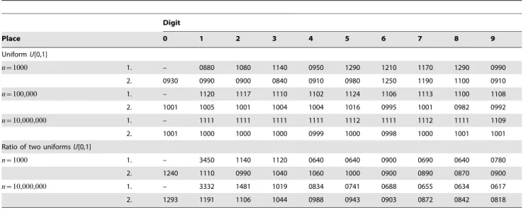
Results
The numerical results for theuniform distributionand the ratio distribution of two uniforms are shown in Table 2. The uniform distribution produces a uniform distribution of first- and second place digits, as was to be expected. Hence, the clear conclusion is, that the uniform distribution and the NBL are incompatible. Nevertheless it is instructive to consider in more detail the discrepancies between the simulated relative frequencies of the digits and their theoretical values to get an impression of the precision which can be expected from the simulation study. Assuming a uniform distribution, the probabilities of occurrence for the first-place digits are1=9and for the second-place digits they are1=10. For the first-place digit, the deviation of the simulated relative frequencies from these values does not exceed .0231 for n~1000and .0013 forn~100,000, respectively. Similar maximal discrepancies (.0250 forn~1000and .0018 for n~100,000) are obtained for the second-place digit. Nearly perfect agreement is
Figure 2. Three distributions of the ratio of two random variables.Ratio distribution of two uniforms U(0,1), ratio distribution of two
found for the first two digits andn~10,000,000, that is, under this sample size the true distribution is generated nearly perfectly. Across all sample sizes, for each digit a its simulated relative frequencyr(a)lies within the approximate (for the number of tests corrected overall) 99% confidence interval around the corre-sponding probabilityp(a), CI:p(a)+3:3 ffiffiffiffiffiffiffiffiffiffiffiffiffiffiffiffiffiffiffiffiffiffiffiffiffiffiffiffiffiffiffi
p(a) 1½ {p(a)=n p
. From this it can be concluded that the pseudo-random number generator works properly. Therefore, rather reliable results can
be expected for all distributions under study even forn~1000in terms of absolute differences between simulated and true distribu-tions. But in terms of relative differences Dr(a){p(a)D=p(a), the agreement must be expected to be much weaker: the maximal relative differences turn out to be 20.29% for n~1000 and 1.17% for n~100,000 in the case of the first-place digit, and 25.00% for n~1000 and 1.80% for n~100,000in the case of the second-place digit. One has to bear in mind these facts when Table 2.Uniform distribution and ratio of two uniforms.
Digit
Place 0 1 2 3 4 5 6 7 8 9
UniformU[0,1]
n~1000 1. – 0880 1080 1140 0950 1290 1210 1170 1290 0990
2. 0930 0990 0900 0840 0910 0980 1250 1190 1100 0910
n~100,000 1. – 1120 1117 1110 1102 1124 1106 1113 1100 1108
2. 1001 1005 1001 1004 1004 1016 0995 1001 0982 0992
n~10,000,000 1. – 1111 1111 1111 1111 1112 1111 1112 1111 1109
2. 1001 1000 1000 1000 0999 1000 0998 1000 1001 1001
Ratio of two uniformsU[0,1]
n~1000 1. – 3450 1140 1120 0640 0640 0900 0690 0640 0780
2. 1240 1110 0990 1040 1060 1000 0900 0890 0870 0900
n~10,000,000 1. – 3332 1481 1019 0834 0741 0688 0655 0634 0617
2. 1293 1191 1106 1044 0988 0943 0903 0872 0842 0818
doi:10.1371/journal.pone.0010541.t002
Table 3.Exponential distribution and ratio of two exponentials.
Digit
Place 0 1 2 3 4 5 6 7 8 9
Exponentialðl~1=2Þ
n~1000 1. – 2900 2010 1200 1030 0690 0800 0380 0480 0510
2. 1160 1230 0890 0970 1040 1080 0970 0870 0990 0800
n~10,000,000 1. – 2971 1945 1353 0987 0757 0612 0516 0451 0408
2. 1171 1122 1082 1041 1008 0974 0943 0914 0885 0860
Exponentialðl~1Þ
n~1000 1. – 3210 1720 1180 0990 0910 0540 0580 0320 0550
2. 1230 1050 1160 1270 1100 0840 0850 0880 0770 0850
n~10,000,000 1. – 3298 1744 1128 0860 0725 0642 0582 0532 0489
2. 1210 1153 1100 1051 1006 0964 0929 0893 0862 0833
Exponentialðl~2Þ
n~1000 1. – 2900 1900 1120 0870 0810 0900 0550 0520 0430
2. 1120 1120 1000 1010 0890 1030 1110 0920 0870 0930
n~10,000,000 1. – 2872 1585 1225 1020 0869 0744 0641 0558 0486
2. 1212 1147 1089 1041 0999 0961 0928 0899 0873 0851
Ratio of two exponentials with parametersl1~l2
n~1000 1. – 3160 1560 1370 0970 0740 0730 0460 0470 0540
2. 1180 1290 1080 1070 1020 0900 0980 0790 0770 0920
n~10,000,000 1. – 3021 1752 1244 0965 0791 0670 0582 0516 0460
2. 1198 1140 1088 1044 1004 0968 0933 0903 0873 0849
evaluating the fit to the NBL in the presence of real data with moderate sample size, as well as when interpreting the results for the various distributions in the following.
In contrast to the uniform distribution, theratio distribution of two uniformsfits the NBL rather good. Forn~10,000,000
the maximal absolute difference between the simulated relative frequencies and the probabilities according to the NBL amounts to .0322, is found for the leading digit 1, and corresponds to a relative difference of 10.7%. For the same sample size even larger relative differences are found in some cases. For example, for the leading digit to be 9, the absolute difference is .0159 only, however resulting in the relative difference of nearly 35%. Especially for the large sample size most of the simulated relative frequencies fall outside any usual confidence interval around the digits’ probabil-ities as given by the NBL. Thus, the NBL does not hold in a strict sense for the ratio distribution of two uniforms, that is, for unrealistically large sample sizes the H0: ‘‘The digits’ distributions follow the NBL’’ would have to be rejected. But the NBL approximates the digits’ distributions to such a degree that it may
be acceptable as a H0 in the presence of real data sets with typical sample size.
The numerical results for theexponential distributionwith parameter l= 0.5, 1, 2 and the ratio distribution of two exponentials are given in Table 3. The exponential distribution produces first- and second-place digits’ distributions coming close to the Newcomb-Benford distribution. As derived theoretically by Engel and Leuenberger [17] and also shown numerically by Leemis, Schmeiser and Evans [18], however for the leading digit only, the maximal absolute deviation is less than 0.03. This result was reproduced here, and it does not only apply to large samples, but also to the sample size ofn~1000. Further, it generalizes to the second-place digit. Note that for both the first- and second place the quality of fit depends onland varies across the digits.
The ratio distribution of two exponentials withl1~l2 clearly outperforms these results. For n~1000, the maximal absolute deviation amounts to .0150 for the first-place digit to be 1 and to .0151 for the second-place digit also to be 1; for n~10,000,000, the maximal deviation is found to be .0011
Table 4.Half-normal distribution and ratio of two half-normals.
Digit
Place 0 1 2 3 4 5 6 7 8 9
Half-normal (s~1)
n~1000 1. – 3800 1190 0800 0680 0640 0750 0810 0850 0480
2. 1270 1120 0930 1200 0940 0930 0970 0920 0960 0760
n~10,000,000 1. – 3636 1279 0850 0803 0769 0732 0687 0644 0600
2. 1263 1190 1124 1062 1007 0954 0907 0864 0830 0798
Half-normal (s~2:5)
n~1000 1. – 2880 2390 1620 1120 0500 0480 0320 0300 0390
2. 1100 1160 1080 0980 0900 1050 1090 0860 0810 0970
n~10,000,000 1. – 2991 2299 1579 1002 0638 0450 0370 0341 0330
2. 1135 1104 1075 1043 1012 0984 0956 0926 0894 0870
Half-normal (s~5)
n~1000 1. – 1990 1320 1560 1330 1060 0880 0740 0630 0490
2. 1220 1010 1100 1180 0980 0900 0950 0780 0950 0930
n~10,000,000 1. – 2129 1572 1419 1243 1056 0873 0706 0559 0443
2. 1196 1116 1059 1016 0984 0962 0940 0923 0908 0897
Ratio of two half-normals withs1~s2
n~1000 1. – 3170 1590 1110 0880 0820 0660 0650 0530 0590
2. 1370 1240 0980 0940 1070 0870 0960 0830 0990 0750
n~10,000,000 1. – 3099 1685 1182 0938 0787 0683 0604 0539 0484
2. 1211 1149 1094 1045 1001 0963 0928 0897 0868 0842
Ratio of two half-normals withs1~2ands2~1
n~1000 1. – 3250 2000 1170 0840 0750 0590 0520 0490 0390
2. 1100 1360 1140 0940 0960 0870 0990 0890 0810 0940
n~10,000,000 1. – 3097 1845 1254 0936 0749 0632 0550 0491 0447
2. 1190 1136 1089 1045 1005 0970 0935 0906 0876 0848
Ratio of two half-normals withs1~1ands2~2
n~1000 1. – 2700 1700 1310 1120 1060 0660 0510 0430 0510
2. 1260 1130 0950 1020 0920 0970 0890 1110 0920 0830
n~10,000,000 1. – 2866 1725 1287 1023 0838 0699 0594 0515 0453
2. 1195 1136 1083 1041 1001 0968 0933 0906 0880 0857
(first-place digit 1). Most simulated relative frequencies look as if they were generated under the NBL, and they lie within the confidence intervals introduced above, except forn~10,000,000. Comparable results were obtained for some ratio distributions of exponentials withl1=l2, but details will be omitted.
The numerical results for thehalf-normal distributionwith
s= 1, 2.5, 5 and the ratio distribution of two half-normals are shown in Table 4. The three half-normals under investigation do not fit the NBL as well as was to be expected following Du¨mbgen and Levenberger [26], but far better than given by Furry and Hurwitz [6]. According to our results, the maximal deviance across all cases studied is found to be .0790 for the first-place digit to be 1 ifs= 1 andn~1000, whereas Furry and Hurwitz reported .33. (Note that Furry and Hurwitz speak of the normal distribution, in fact they investigated the half-normal, as can be seen from their formula (a) on p.53. Note further that they reported .115 for the deviance of the exponential distribution – which now is known to be much smaller, see above –, but .0557 for the half Cauchy distribution that was not included in the present study because of its similarity with the normal distribution; cf. thereto p.300 in Johnson, Kotz and Balakrishnan [39]). The digits’ distributions remain unaffected when multiplyingsby integer powers of 10 so that, for example, the entries found in the first half of Table 4 also apply to the half-normal withs= 10,s= 25, ands= 50, respectively.
Surprisingly good fit to the NBL shows theratio distribution of two half-normalswiths1~s2(independent of their actual values),s1~2,s2~1, ands1~1,s2~2. The fit is not as perfect as it is for the ratio of two exponentials, but it is better than that of the ratio of two uniforms. Especially good agreement is observed for the second-place digit under all three scenarios studied here, and even for the first-place digit the maximal deviance is found to be only .0089, .0087, and .0256, respectively (digit 1, n~10,000,000). Overall, it seems to make little difference of whether the variances of the two random variables are equal or not, with the slight tendency to worsen the fit if the variance of the variable in the denominator,Y, exceeds that of the numerator,X, in the ratioZ~X=Y.
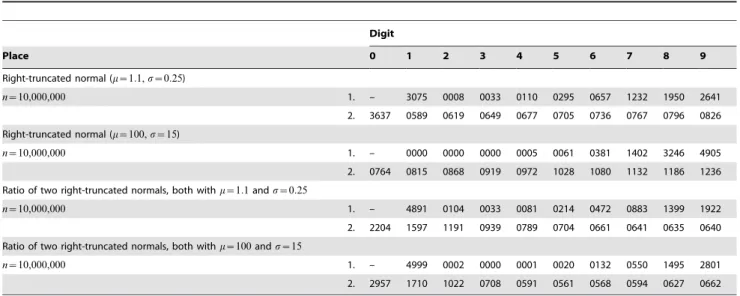
The numerical results for the right-truncated normal distribution and the ratio distribution of two right-truncated normals are given in Table 5. Its entries speak for themselves so that a short comment will suffice. As compared with
survival distributions, the right-truncated normal shows inverse behaviour in that it puts most mass on large values of the random variable. That is why the right-truncated normal was selected for inclusion in the present study. It turns out that it may serve as a prototypical example of distributions of random variables not leading to first- and second-place digits’ distributions obeying the NBL. Presented are the figures only for n~10,000,000, two distributions, withm= 1.1,s= 0.25 andm= 100,s= 15, and their ratio distributions. The discrepancies between the simulated digits’ distributions and the Newcomb-Benford distribution are such that even for small sample sizes conventional goodness-of-fit tests, for example Pearson’s chi-square and the likelihood-ratio test, have a good chance to become significant. Considering the ratio distribution of two right-truncated normals does not improve matters. (Note that nonconformance to the NBL was reported for the Gumbel distribution whose density also increases with increasing value of the random variable [26].)
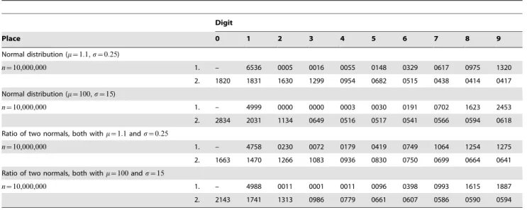
Similar results were obtained for the normal distribution and theratio distribution of two normals; see Table 6. The normal distribution, putting most mass around the mean of the random variable, was selected for inclusion in the present study as a further possible candidate of nonconformity with the NBL. Neither the normal distribution nor the ratio distribution of two normals disappointed this expectation. As for the right-truncated normal, figures are presented forn~10,000,000and two sets of parameters only.
The numerical results for the chi-square distribution and the ratio distribution of two chi-squares are shown in Table 7. Regarding the chi-square distribution, a clear tendency becomes obvious. Very good fit to the NBL is found for the chi-square withdf~1(n~10,000,000, maximal deviance .0065 for first-place digit 2), increasing thedf (shown fordf~2and df~5) worsens the fit considerably. This does not come as a surprise when taking the shape of the square distribution into account: the chi-square with df~1 behaves like a survival distribution, for increasingdf it approaches a normal distribution.
The ratio distribution of two chi-squares (F -distribu-tion) with df1~df2~df fits better than does the chi-square. Moreover, the ratio distribution of two chi-squares proves more robust against increasing thedf. For df~1, the simulated first-and second-place digits’ distributions are nearly indistinguishable
Table 5.Right-truncated normal distribution and ratio of two right-truncated normals.
Digit
Place 0 1 2 3 4 5 6 7 8 9
Right-truncated normal (m~1:1,s~0:25)
n~10,000,000 1. – 3075 0008 0033 0110 0295 0657 1232 1950 2641
2. 3637 0589 0619 0649 0677 0705 0736 0767 0796 0826
Right-truncated normal (m~100,s~15)
n~10,000,000 1. – 0000 0000 0000 0005 0061 0381 1402 3246 4905
2. 0764 0815 0868 0919 0972 1028 1080 1132 1186 1236
Ratio of two right-truncated normals, both withm~1:1ands~0:25
n~10,000,000 1. – 4891 0104 0033 0081 0214 0472 0883 1399 1922
2. 2204 1597 1191 0939 0789 0704 0661 0641 0635 0640
Ratio of two right-truncated normals, both withm~100ands~15
n~10,000,000 1. – 4999 0002 0000 0001 0020 0132 0550 1495 2801
2. 2957 1710 1022 0708 0591 0561 0568 0594 0627 0662
Table 6.Normal distribution and ratio of two normals.
Digit
Place 0 1 2 3 4 5 6 7 8 9
Normal distribution (m~1:1,s~0:25)
n~10,000,000 1. – 6536 0005 0016 0055 0148 0329 0617 0975 1320
2. 1820 1831 1630 1299 0954 0682 0515 0438 0414 0417
Normal distribution (m~100,s~15)
n~10,000,000 1. – 4999 0000 0000 0003 0030 0191 0702 1623 2453
2. 2834 2031 1134 0649 0516 0517 0541 0566 0594 0618
Ratio of two normals, both withm~1:1ands~0:25
n~10,000,000 1. – 4758 0230 0072 0179 0419 0749 1064 1254 1275
2. 1663 1470 1266 1083 0936 0830 0750 0699 0664 0641
Ratio of two normals, both withm~100ands~15
n~10,000,000 1. – 4988 0011 0001 0011 0096 0398 0993 1615 1887
2. 2143 1741 1313 0986 0779 0661 0607 0586 0590 0594
doi:10.1371/journal.pone.0010541.t006
Table 7.Chi-square distribution and ratio of two chi-squares (F-distribution).
Digit
Place 0 1 2 3 4 5 6 7 8 9
Chi-square (df~1)
n~1000 1. – 3050 1840 1250 0850 0760 0820 0600 0500 0330
2. 1330 1050 1070 1000 0950 0960 0960 0920 0820 0940
n~10,000,000 1. – 3071 1826 1257 0949 0759 0639 0556 0495 0448
2. 1192 1138 1087 1045 1006 0968 0936 0905 0874 0849
Chi-square (df~2)
n~1000 1. – 2810 2090 1220 1020 0960 0620 0420 0520 0340
2. 1200 1320 1270 0990 0860 0970 0960 0940 0850 0640
n~10,000,000 1. – 2961 1959 1365 0993 0757 0607 0511 0445 0402
2. 1168 1121 1079 1041 1007 0974 0944 0915 0888 0862
Chi-square (df~5)
n~1000 1. – 1820 1580 1530 1440 1020 1080 0520 0480 0530
2. 1220 1210 1040 0880 0960 0940 1140 0880 0840 0890
n~10,000,000 1. - 1820 1494 1532 1383 1159 0927 0720 0547 0418
2. 1183 1107 1052 1010 0983 0961 0945 0930 0920 0909
Ratio of two chi-squares, both withdf~1
n~1000 1. – 3160 1510 1470 0770 0780 0770 0610 0450 0480
2. 1170 1340 1100 1090 0960 0840 0950 0860 0880 0810
n~10,000,000 1. – 3013 1760 1249 0969 0791 0667 0581 0512 0458
2. 1196 1140 1089 1042 1003 0967 0935 0903 0874 0850
Ratio of two chi-squares, both withdf~2(see ratio of two exponentials, Table 3)
Ratio of two chi-squares, both withdf~5
n~1000 1. – 3100 1610 1110 1090 0740 0670 0590 0520 0570
2. 1030 1280 0990 1070 1050 1000 1070 0880 0870 0760
n~10,000,000 1. – 3180 1619 1119 0907 0784 0698 0624 0562 0507
2. 1221 1157 1100 1046 1004 0960 0924 0892 0860 0835
from the Newcomb-Benford distribution, and up to df~5 the deviance increases rather slowly. Note that theF-distribution with
df1~df2~2is formally identical to the ratio distribution of two exponentials with l1~l2. Therefore, figures for F(2,2) were omitted; see Table 3.
The numerical results for thelog-normal distribution are given in Table 8. For this two-parameter distribution, the fit to the NBL heavily depends onsand slightly depends onm. The largers
and/orm, the better is the fit. Form~0,s~1andm~:33,s~1
the misfit is massive, so that considering the effect of sample size becomes obsolete; hence figures are given forn~10,000,000only. The best fit amongst the cases reported here is obtained with
m~10, s~40: the simulated first- and second-place digits’ distributions come very close to the Newcomb-Benford distribu-tion when n~10,000,000; the maximal deviance amounts to .0064 and refers to the first-place digit 1. As the ratio distribution of two log-normals also follows the log-normal, no separate presentation of results is needed.
The results of the simulation study may be summarized in two statements. First, all types of distributions which turned out to be compatible with the NBL exhibit a common feature. They are long right-tailed and, thus, put most mass on small values of the random variable. To these distributions belong the exponential, the chi-square with very small degrees of freedom (df~1 and
df~2), the log-normal with large variance, and, with some limitations, the half-normal. Incompatibility with the NBL proved the uniform, the normal, and the right-truncated normal distributions. Second, the fit to the NBL generally improves when considering distributions of ratios of random variables. Among the seven types of ratio distributions studied here, five emerged as being consistent with the NBL. The ratio distribution of two exponentials, the ratio distribution of two chi-squares (F
-distribution) with small degrees of freedom, and the ratio distribution of two log-normals with large variance fitted the first-and second-place digits’ distributions as given by the NBL nearly perfectly, the ratio distributions of two uniforms and of two half-normals fitted it sufficiently well, whereas only the ratio distributions of two normals and of two right-truncated normals completely failed to fit.
Together with findings reported earlier [6,17,18,26] regarding the conformance to the NBL for some survival distributions (exponential, Muth, Gompertz, Weibull, gamma, log-logistic, and exponential power distributions) our results indicate that the validity of the NBL requires that the frequency of ‘natural’ numbers in the sense of Newcomb [1] decreases with increasing magnitude. Roughly speaking, this means that small numbers have to be predominant. That is, when thinking of real-world data, conformity to the NBL necessitates a majority of small objects. As
Table 8.Log-normal distribution.
Digit
Place 0 1 2 3 4 5 6 7 8 9
Log-normal (m~0,s~1)
n~10,000,000 1. – 6931 3069 0000 0000 0000 0000 0000 0000 0000
2. 1442 1335 1246 1167 1098 1037 0983 0639 0541 0512
Log-normal (m~0:33,s~1)
n~10,000,000 1. – 3599 4054 2346 0000 0000 0000 0000 0000 0000
2. 0816 0782 0752 0756 1387 1320 1256 1186 0893 0853
Log-normal (m~0,s~10)
n~1000 1. – 3520 1680 1290 0980 0700 0590 0460 0440 0340
2. 1200 1040 1160 1100 1080 1040 0840 0870 0880 0790
n~10,000,000 1. – 3466 1719 1151 0893 0729 0616 0534 0472 0420
2. 1248 1181 1083 1034 0994 0954 0922 0889 0861 0834
Log-normal (m~2:5,s~10)
n~1000 1. – 3270 1690 1380 0940 0780 0600 0560 0390 0390
2. 1130 1150 0970 0990 0880 1040 1020 1000 0860 0960
n~10,000,000 1. – 3268 1915 1152 0892 0729 0617 0533 0471 0422
2. 1151 1093 1112 1077 1034 0995 0953 0890 0861 0835
Log-normal (m~0,s~40)
n~1000 1. – 2940 1710 1360 1010 0750 0780 0490 0450 0510
2. 1250 1240 1230 1100 0930 0900 0930 0980 0740 0700
n~10,000,000 1. – 3118 1764 1222 0951 0775 0655 0566 0501 0448
2. 1206 1148 1096 1046 0997 0963 0929 0899 0871 0844
Log-normal (m~10,s~40)
n~1000 1. – 2940 1900 1150 0890 0740 0690 0680 0510 0500
2. 1380 1270 1020 1050 1100 0970 0730 0840 0890 0750
n~10,000,000 1. – 2946 1801 1294 1003 0785 0654 0567 0501 0449
2. 1190 1133 1089 1047 1004 0967 0935 0907 0877 0852
the NBL has often been shown to be valid, conversely it can be deduced that, at least within numerous domains of our world, small objects must occur much more frequently than do large ones. Some examples given in the following will sustain this conclusion.
Analyzed were the distributions of the following five variables plus their first- and second-place digits’ distributions.
(a) The closing prices in Euro as of June 30, 2009 of stocks contained in the AEX (Netherlands), ATX (Austria), CAC40 (France), DAX (Germany), DJI (USA), DJStoxx50 (Europe) and SMI (Swiss), in total 179 values whereby stocks entered only once when they appeared twice, namely in one of the local European stock indices and in the overall European index DJStoxx50;
(b) the closing prices of these stocks, however in local currencies (Euro, US-$, Swiss Franc);
(c) the areas of 198 countries;
(d) the numbers of inhabitants of these 198 countries; and (e) the starting page numbers of 225 papers referenced in the
bibliography on the NBL compiled by Hu¨rlimann [7].
Overall, results are as expected. First, all five variables possess a marked majority of small and a clear minority of large realizations. Four of the five variables exhibit a distribution coming more (areas and inhabitants of countries) or less (stock prices: very low values are underrepresented) close to survival distributions. The distri-bution of one variable (the bibliography data) follows rather a step function than a continuously decreasing density function: the highest frequency is found for starting pages 1 to 99 as it was to be expected; the starting pages 100 to 199, 200 to 299, and 300 to 399 occur with markedly lower, but approximately constant frequency; then the frequency decreases sharply to a level remaining approximately constant for the following five 100-pages sections (Figure 3; frequency distributions on the left).
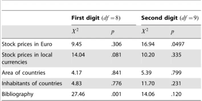
Second, in all five cases the first-place digit 1 is slightly underrepresented. Nevertheless, based on the Pearson chi-squared goodness-of-fit test (5% significance level), all of the first- and second-place digits’ distributions are compatible with the NBL, with one exception: the first-place digit’s distribution of the bibliography data clearly fails to fit the NBL; see Table 9. The best fit is found for the areas of countries and their numbers of inhabitants, weaker fit is found for both variants of stock prices (prices in Euro vs. prices in local currencies). Note that the second-place digit’s distribution of the stock prices in Euro is a borderline case pointing at the importance not to look at the first-place digit only when testing for the fit of the NBL. The first- and second-place digits’ distributions are shown in Figure 3 on the right, whereby observed values are represented by bars, values expected according to the NBL by a line.
Third, and most importantly, the examples demonstrate the link between the distribution of a random variable on the one hand and the first-and second place digits’ distributions on the other hand. The closer the shape of the distribution of a random variable comes to that of a survival distribution or a distribution behaving like a survival distribution, the better follows the first-and second-place digits’ distributions the NBL. Regarding our five examples, the same ordering according to both properties is
observable: the areas of countries and their numbers of inhabitants perform best, both versions of stock prices perform to some extent, but the bibliography data do simply not.
Discussion
In the first part of this study seven types of common distributions were investigated regarding their conformance to the NBL. The results of the simulations showed first that all types of distributions behaving like survival distributions, that is, putting most mass on small values of the random variable and being long right-tailed, were compatible with the NBL. Second, distributions of the ratio of two random variables fitted better than did the distributions of a single random variable. For symmetric distributions (illustrated by example of the normal distribution), distributions tending to symmetry as a function of their parameters (illustrated by example of the chi-square and the log-normal distributions), and distributions whose density increases with increasing value of the random variable (illustrated by example of the right-truncated normal distribution), the misfit to the NBL was found to be substantial up to massive.
These observations together with the fact that the NBL – at least approximately – applies to many empirical data led to the suspicion that the size of ‘natural’ objects must follow a distribution behaving like a survival distribution in order to be able to obey the NBL. This suspicion could be substantiated by analyzing five sets of data. It turned out that the closer the distribution of a variable comes to that of a survival distribution the better is the fit to the NBL. Thereby, the fit to the NBL was tested formally by chi-square goodness-of-fit tests of the first- and second-place digits’ distributions, whereas the fit of the observed variable’s distribution to a survival distribution of unspecified form was informally assessed by visual inspection.
The overall conclusion resulting from the present study reads very simply. The frequently found good fit of the NBL to empirical data can be explained by the fact that in many cases the frequency with which objects occur in ‘nature’ is an inverse function of their size. Very small objects occur much more frequently than do small ones which in turn occur more frequently than do large ones and so on. Thus, the variable’s distribution looks like a survival distribution whose leading digits’ distributions follow the NBL, at least approximately.
Figure 3. Five empirical examples.Stock prices in Euro, stock prices in local currencies, area of countries (in units of 100,000 sq.km.), population
of countries (in units of millions), starting page of papers referenced in a bibliography on the Newcomb-Benford law. For each data set, the distribution of the observed variable is shown on the left, the resulting first- and second-place digits’ distributions are shown on the right (bars) together with the respective distributions according to the Newcomb-Benford law (solid lines).
doi:10.1371/journal.pone.0010541.g003
Table 9.Results of the Pearson chi-square tests for the five empirical examples.
First digit(df~8) Second digit(df~9)
X2 p X2 p
Stock prices in Euro 9.45 .306 16.94 .0497
Stock prices in local currencies
14.04 .081 10.20 .335
Area of countries 4.17 .841 5.39 .799
Inhabitants of countries 4.83 .776 11.70 .231
Bibliography 27.46 .001 14.06 .120
It is somewhat surprising that in the literature on the NBL the connection between the distribution of a random variable and the leading digits’ distributions was investigated up to now only for a handful of mainly survival distributions. Studies referring to empirical data concentrated solely on the leading digits’ distributions, nearly always on the most significant digit only, neither discussing the relationship between the leading digits’ distributions and the variable’s distribution nor presenting the latter one. As a consequence, reanalyzing empirical data collected earlier was not possible and new data had to be found. Presumably the present study is therefore the first one focusing on the connection between the variables’ distribution and the leading digits’ distributions, in both theoretical and empirical settings. It remains to hope that future investigations on and applications of the NBL will pursue the approach taken here.
Acknowledgments
The author wishes to thank the Scientific Editor, Dr. Richard J. Morris, and an anonymous referee for their comments and suggestions that improved the completeness and presentation of this article. The author is especially grateful to Professor Theodore P. Hill, who also acted as a referee, for a very helpful discussion that clarified some critical issues arising from the literature. For having professionally prepared the figures, the author is indebted to Dipl.Ing. Martina Edl and Mike Swazina.
Author Contributions
Conceived and designed the experiments: AKF. Performed the experi-ments: AKF. Analyzed the data: AKF. Contributed reagents/materials/ analysis tools: AKF. Wrote the paper: AKF.
References
1. Newcomb S (1881) Note on the frequency of use of the different digits in natural numbers. Am J Math 4: 39–40.
2. Benford F (1938) The law of anomalous numbers. Proc Am Phil Soc 78: 551–572.
3. Raimi RA (1976) The first digit problem. Am Math Mon 83: 521–538. 4. Pinkham RS (1961) On the distribution of first significant digits. Ann Math Stat
32: 1223–1230.
5. Knuth DE (1997) The art of computer programming. Vol.2, 3rd edition. Reading, MA: Addison-Wesley.
6. Furry WH, Hurwitz H (1945) Distribution of numbers and distribution of significant figures. Nature 155: 52–53.
7. Hu¨rlimann W (2006) Benford’s law from 1881 to 2006: A bibliography. www. geocities.com/hurlimann53.
8. Berger A, Hill TP (2010) Benford online bibliography. www.benfordonline.net. 9. Hill TP (1995) Base-invariance implies Benford’s law. Proc Am Math Soc 123:
887–895.
10. Hill TP (1995) The significant-digit phenomenon. Am Math Mon 102: 322–327. 11. Hill TP (1995) A statistical derivation of the significant-digit law. Stat Sci 10:
354–363.
12. Schatte P (1996) On Benford’s law to variable base. Stat Probabil Lett 37: 391–397.
13. Lolbert T (2008) On the non-existence of a general Benford’s law. Math Soc Sci 55: 103–106.
14. Irmay S (1997) The relationship between Zipf’s law and the distribution of first digits. J Appl Stat 24: 383–393.
15. Luque B, Lacasa L (2009) The first digit frequencies of prime numbers and Riemann zeta zeroes. P Roy Soc A-Math Phy 465: 2197–2216.
16. Miller SJ, Nigrini MJ (2008) Order statistics and Benford’s law. arxiv:math/ 0601344v5.
17. Engel H-A, Leuenberger C (2003) Benford’s law for exponential random variables. Stat Probabil Lett 63: 361–365.
18. Leemis LM, Schmeiser BW, Evans DL (2000) Survival distributions satisfying Benford’s law. Am Stat 54: 236–241.
19. Rodriguez RJ (2004) First significant digit patterns from mixtures of uniform distributions. Am Stat 58: 64–71.
20. Janvresse E´ , De la Rue T (2004) From uniform distributions to Benford’s law. J Appl Probab 41: 1203–1210.
21. Gottwald GA, Nicol M (2002) On the nature of Benford’s law. Physica A 303: 387–396.
22. Pietronero L, Tosatti E, Tosatti V, Vespignani A (2001) Explaining the uneven distribution of numbers in nature: the laws of Benford and Zipf. Physica A 293: 297–304.
23. Torres J, Fernandez S, Gamero A, Sola A (2007) How do numbers begin ? (The first digit law). Eur J Phys 28: L17–L25.
24. Adhikari AK, Sarkar BP (1968) Distribution of most significant digit in certain functions whose arguments are random variables. Sankhya B 30: 47–58. 25. Adhikari AK (1969) Some results on the distribution of most significant digit.
Sankhya B 31: 413–420.
26. Du¨mbgen L, Leuenberger C (2008) Explicit bounds for the approximation error in Benford’s law. Elect Comm in Probab 13: 99–112.
27. Ley E (1996) On the peculiar distribution of the US stock indexes’ digits. Am Stat 50: 311–313.
28. Hill TP (1998) The first digit phenomenon. Am Sci 86: 358–363.
29. Giles DE (2007) Benford’s law and naturally occurring prices in certain ebay auctions. App Econ Lett 14: 157–161.
30. el Sehity T, Hoelzl E, Kirchler E (2005) Price developments after a nominal shock: Benford’s law and psychological pricing after the euro introduction. Int J Res Mark 22: 471–480.
31. Nigrini MJ (2000) Digital analysis using Benford’s law. Vancouver: Global Audit Publications.
32. Judge G, Schechter L (2009) Detecting problems in survey data using Benford’s law. J Hum Resour 44: 1–24.
33. Hales DN, Sridharan V, Radhakrishnan A, Chakravorty SS, Siha SM (2008) Testing the accuracy of employee-reported data: an inexpensive alternative approach to traditional methods. Eur J Oper Res 189: 583–593.
34. Diekmann A (2007) Not the first digit! Using Benford’s law to detect fraudulent scientific data. J Appl Stat 34: 321–329.
35. Browne MW (1998) Following Benford’s law, or looking out for no. 1. The New York Times, August 4, 1998.
36. Beer TW (2009) Terminal digit preference: beware of Benford’s law. J Clin Pathol 62: 192.
37. Kim H-J (2006) On the ratio of two folded normal distributions. Commun Stat– Theor M 35: 965–977.
38. Hinkley DV (1969) On the ratio of two correlated normal random variables. Biometrika 56: 635–639.