Tackling the Protein Folding Problem by a
Generalized-Ensemble Approach with Tsallis Statistics
Ulrich H.E. Hansmann
a;and Yuko Okamoto
b; y aDepartment of PhysicsMichigan Technological University Houghton, MI 49931-1291, U.S.A.
b Department of Theoretical Studies
Institute for Molecular Science
and
Department of Functional Molecular Science The Graduate University for Advanced Studies
Okazaki, Aichi 444-8585, Japan
Received 07 December, 1998
We review uses of Tsallis statistical mechanics in the protein folding problem. Monte Carlo simu-lated annealing algorithm and generalized-ensemble algorithm with both Monte Carlo and stochastic dynamics algorithms are discussed. Simulations by these algorithms are performed for a penta pep-tide, Met-enkephalin. In particular, for generalized-ensemble algorithms, it is shown that from only one simulation run one can nd the global-minimum-energy conformation and obtain probability distributions in canonical ensemble for a wide temperature range, which allows the calculation of any thermodynamic quantity as a function of temperature.
I. Intro duction
For many important physical systems like biolog-ical macromolecules it is very dicult to obtain the accurate canonical distribution at low temperatures by conventional simulation methods. This is because the energy function has a huge number of local minimasep-arated by high energy barriers, and at low temperatures simulations will necessarily get trapped in the cong-urations corresponding to one of these local minima. In order to overcome this multiple-minima problem, many methods have been proposed. Simulated anneal-ing [1] is probably the most widely used algorithm that can alleviate the diculty. Generalized-ensemble algo-rithms, most well-known of which is the multicanonical approach [2, 3], are also powerful ones, and were rst introduced to the protein-folding problem in Ref. [4]. Simulations in the multicanonical ensemble perform 1D random walk in energy space, which allows the
sys-tem to overcome any energy barrier. Besides multi-canonical algorithms, simulated tempering [5, 6] and 1/k-sampling [7] have been shown to be equally eec-tive generalized-ensemble methods in the protein fold-ing problem [8]. The simulations are usually performed with Monte Carlo (MC) scheme, but recently molecu-lar dynamics (MD) version of multicanonical algorithm was also developed [9]-[11].
The generalized-ensemble approach is based on non-Boltzmann probability weight factors, and in the above three methods the determination of the weight fac-tors is non-trivial. We have shown that a particular choice of the Tsallis weight factor [12] can be used for generalized-ensemble simulations [13, 14]. The advan-tage of this ensemble is that it greatly simplies the determination of the weight factor.
In this article, we review simulated annealing and generalized-ensemble algorithmsbased on Tsallis e-mail: [email protected]
tics. The performances of the algorithms are tested with the system of an oligopeptide, Met-enkephalin.
II. Methods
II.1 Energy Function of Protein Systems
The total potential energy functionE
totfor the pro-tein systems that we used is one of the standard ones. Namely, it is given by the sum of the electrostatic term E
C, 12-6 Lennard-Jones term E
LJ, and hydrogen-bond termE
HBfor all pairs of atoms in the molecule together with the torsion termE
tor for all torsion angles: E P = E C+ E LJ+ E HB+ E tor ; E C = X (i;j) 332q i q j r ij ; E LJ = X (i;j) A ij r 12 ij , B ij r 6 ij ! ; (1) E HB = X (i;j) C ij r 12 ij , D ij r 10 ij ! ; E tor = X i U i ,
1cos(n i i) : Here,r
ij is the distance (in A) between atoms
iandj, is the dielectric constant, and
iis the torsion angle for the chemical bondi. Each atom is expressed by a point at its center of mass, and the partial chargeq
i(in units of electronic charges) is assumed to be concentrated at that point. The factor 332 in E
C is a constant to express energy in units of kcal/mol. These parameters in the energy function as well as the molecular geome-try were adopted from ECEPP/2 [15]. The computer code KONF90 [16] was used for the MC simulations and SMC [17] was used for the MD simulations. We neglected the solvent contributions for simplicity and set the dielectric constant equal to 2. The peptide-bond dihedral angles!were xed at the value 180
for simplicity. So, the remaining dihedral angles and in the main chain and in the side chains constitute the variables to be updated in the simulations. One MC sweep consists of updating all these angles once with Metropolis evaluation [18] for each update.
II.2 Simulated Annealing Algorithm with
Tsal-lis Statistics
In the canonical ensemble at temperatureT each state with potential energyE is weighted by the Boltzmann factor
w B(
E;T) =e , E
; (2)
where the inverse temperature is given by = 1=k B
T with Boltzmann constantk
B. This weight factor gives the usual bell-shaped canonical probability distribution of energy:
P B(
E;T)/n(E)w B(
E;T); (3)
where n(E) is the density of states. For systems with many degrees of freedom, it is usually very dicult to generate a canonical distribution at low temperatures. This is because there are many local minima in the en-ergy function, and simulations will get trapped in states of these local minima.
A now almost classical way to alleviate this di-culty is simulated annealing [1]. Its underlying idea of modeling the crystal grow process in nature is easy to understand and simple to implement. Any MC or MD technique can be converted into a simulated annealing algorithm in a straightforward manner. During a sim-ulation temperature is lowered very slowly from a su-ciently high initial temperatureT
I where the structure changes freely with MC or MD updates to a \freez-ing" temperature T
F where the system undergoes no signicant changes with respect to the MC sweeps or MD steps. If the rate of temperature decrease is slow enough for the system to stay in thermodynamic equi-librium, then it is ensured that the system can avoid getting trapped in local minima and that the global minimum will be found.
achieved by a simple cooling process, elaborated and system-specic annealing schedules are often necessary to obtain the global minimum within the CPU time available. In our simulations the temperature was low-ered exponentially in NS (number of total MC sweeps) steps by setting the inverse temperature = 1=kBT at k-th MC sweep to [16, 20]
k=Ik ,1
: (4)
Here,I is the initial inverse temperature andis given in terms of initial and nal temperatures by
=
F I
1 N
S ,1
=
TI TF
1 N
S ,1
: (5)
For a xed value of the total MC sweepsNS, the initial and nal temperatures (TIandTF) are free parameters and have to be tuned in such a way that the annealing process is optimized for the specic problem.
Simulated annealing was rst successfully used to predict the global minimum-energy conformations of polypeptides and proteins in Refs. [21]-[23] and to re-ne protein structures from NMR and X-ray data in Refs. [24, 25]. Since then many promising results have been obtained. Latest applications include Refs. [26]-[29].
Attempts have been made to improve the perfor-mance of simulated annealing in practical applications, see for instance Refs. [30, 20, 8]. More recent attempts [31]-[34] are inspired by Tsallis generalized statistical mechanics [12].
In the Tsallis formalism [12], a generalized statisti-cal mechanics is constructed by maximizing a general-ized entropy
S=,kB 1,
P
ip
q i
q,1
(6) with the constraints
X
i
pi= 1 ;
X
i
pqiEi= const: (7) Here, q is a real number. A generalized probability weight
w(E)/[1 + (q,1)E] ,
1
q ,1 (8)
follows, which tends to the Boltzmann factor of Eq. (2) forq!1, and therefore regular statistical mechanics is recovered in this limit. The important feature of Tsallis
generalized statistical mechanics for optimization prob-lems is that the probability distribution of energy does no longer decrease exponentially with energy but ac-cording to a power law, where the exponent is deter-mined by the free parameter q (compare Eqs. (2) and (8)). The resulting probability distribution has a tail to higher energies for q > 1, which enhances the ex-cursion into high-energy regions and escape from local-minimum states.
This observation inspired the construction of vari-ous generalized simulated annealing algorithms based on Tsallis weight factors [31]-[34]. As an example we present here the generalized simulated annealing tech-nique proposed in Ref. [34]. The congurations are weighted with
w(E) = [1 + (q,1)(E,EGS)] ,
q q ,1
; (9) where EGS is the ground-state energy and the Tsallis parameter q has been set to be: q = 1 +
1
nF. Here, nF is the number of degrees of freedom. Note that through the substraction ofEGS it is ensured that the weights will always be positive denite. However, in general EGS is not known. We therefore approximate EGS in the course of a simulated annealing simulation by E
0
Emin ,c, where Emin is the lowest energy ever encountered in the simulation andc a small num-ber. E
0 is reset every time a new value for
Emin is found. Changing the value of E
0 is a disturbance of the Markov chain and while we expect the disturbance to be small, we clearly cannot use our algorithm to calculate thermodynamic averages. Moreover, because of the nite step size of the temperature annealing we cannot assume convergence against an equilibrium distribution. As in the regular simulated annealing algorithm, our method is thus valid only as a global optimization method.
II.3 Generalized-Ensemble Algorithm with
Tsallis Statistics
algorithms. Here, we discuss one of the latest exam-ples of simulation techniques in generalized ensemble [13, 14]. The probability weight factor of this method is given by
w(E) =
1 + 0
E,EGS m
,m
; (10)
where T0 = 1=kB0 is a low temperature, EGS is the global-minimum potential energy, and m(> 0) is a free parameter the optimal value of which will be given be-low. This is the Tsallis weight of Eq. (8) at a xed temperature T0with the following choice of q:
q = 1 + 1m : (11)
The above choice of the weight was motivated by the following reasoning [13]. We are interested in an ensem-ble where not only the low-energy region can be sam-pled eciently but also the high-energy states can be visited with nite probability. In this way the simula-tion can overcome energy barriers and escape from local minima. The probability distribution of energy should resemble that of an ideal low-temperature canonical distribution, but with a tail to higher energies. The Tsallis weight of Eq. (10) at low temperature T0 has the required properties when the parameter m is care-fully chosen. Namely, for suitable m > 0 it is a good approximation of the Boltzmann weight wB(E;T0) = exp(,
0(E
,EGS)) for 0(E
,EGS)=m1 , while at high energies it is no longer exponentially suppressed but only according to a power law with the exponent m.
In this work we consider a system with continuous degrees of freedom. At low temperatures the harmonic approximation holds, and the density of states is given by
n(E)/(E,EGS) n
F
2 ; (12)
where nFis the number of degrees of freedom of the
sys-tem under consideration. Hence, by Eqs. (10) and (12) the probability distribution of energy for the present ensemble is given by
P(E)/n(E)w(E)/(E,EGS) n
F 2
,m ; (13) for 0
E,E GS
m 1. This implies that we need m > n F 2 . For, otherwise, the sampling of high-energy congura-tions will be enhanced too much. On the other hand,
in the limit m!1our weight tends for all energies to the Boltzmann weight and high-energy congurations will not be sampled.
In order for low-temperature simulations to be able to escape from energy local minima, the weight should start deviating from the (exponentially damped) Boltz-mann weight at the energy near its mean value (because at low temperatures there are only small uctuations of energy around its mean). In Eq. (10) we may thus set
0
< E >T ,EGS
m = 12 : (14)
The mean value at low temperatures is given by the harmonic approximation:
< E >T = EGS+ n2 kF BT0= EGS+ n
F
20
: (15) Substituting this value into Eq. (14), we obtain the op-timal value for the exponent m:
mopt= nF : (16)
Hence, the optimal weight factor is given by
w(E) =
1 + 0 E,E
0 nF
,n
F
; (17)
where E0 is the best estimate of the global-minimum energy EGS.
We remark that the calculation of the weight factor is much easier than in other generalized-ensemble tech-niques, since it requires one to nd only an estimator for the ground-state energy EGS.
As in the case of other generalized ensembles, we can use the reweighting techniques [35] to construct canon-ical distributions at various temperatures T. This is because the simulation by the present algorithm sam-ples a large range of energies. The thermodynamic av-erage of any physical quantityAcan be calculated over a wide temperature range by
<A>T = Z
dxA(x) w
,1(E(x)) e,E(x) Z
dx w,1(E(x)) e,E(x)
; (18)
Once the weight factor is given, we can implement the Metropolis MC algorithm [18] in a straightforward manner.
We now describe MD algorithm in the new ensem-ble dened by the weight of Eq. (17). We remark that similar stochastic dynamics algorithms were also devel-oped in the context of Tsallis statistical mechanics in Refs. [36, 37].
The classical MD algorithm is based on a Hamilto-nian
H(q ;) = 12 N X i=1 2 i +
E(q 1
;;q N)
; (19) where
i are the conjugate momenta corresponding to the coordinatesq
i. Hamilton's equations of motion are then given by
8 > < > : _ q i = @H @ i = i ; _ i = , @H @q i =, @E @q i = f i ; (20)
and they are used to generate representative ensembles of congurations. For numerical work the time is dis-cretized with a step tand the equations are integrated according to theleapfrog(or other time reversible
inte-gration) scheme: 8 > > < > > : q i(
t+ t) =q i(
t) + t i t+ t 2 ; i
t+ 32t = i t+ t 2 + tf
i(
t+ t): (21) The initial momentaf
i( t
2 )
gfor the iteration are pre-pared by i t 2 =
i(0) + t 2 f
i(0)
; (22)
with appropriately chosenq
i(0) and
i(0) (
i(0) is from a Gaussian distribution).
In order to generalize this widely used technique to simulations in our generalized ensemble, we rewrite the weight factor in Eq. (17) as
w(E) = exp , 0 n F 0 ln 1 + 0 E,E
GS n F ; (23) We then dene an eective potential energy by [36, 37]
E eff(
E) = n F 0 ln 1 + 0 E,E
GS n
F
: (24)
We can see that MD simulations in the new ensemble can be performed by replacingE byE
eff (of Eq. (24)) in Eq. (20). A new set of Hamilton's equations of mo-tion are now given by
c 8 > > < > > : _ q i = i ; _ i = , @E eff @q i =, @E eff @E @E @q i = 1 1 + 0 n F (E,E
GS) f
i
: (25)
d This is the set of equations we adopt for MD simulations in our new ensemble [14]. For numerical work the time is again discretized with a step t and the equations are integrated according to the leapfrogscheme.
Langevin algorithm [38] and hybrid Monte Carlo algorithm [39] in the new ensemble can likewise be in-troduced. It was shown that the performances of these three stochastic dynamics algorithms and that of MC version are similar (for details, see Ref. [14]).
III. Results
III.1 Simulated Annealing Algorithm
The eectiveness of the algorithms presented in the previous section is tested for the system of an oligopep-tide, Met-enkephalin. This peptide has the amino-acid sequence Tyr-Gly-Gly-Phe-Met.
sim-ulated annealing method [34]. As in an earlier work on Met-enkephalin [20] we made 20 runs of 50,000 MC sweeps for various annealing schedules. Each run started from completely random conformations. One of the quantities we monitored to evaluate the perfor-mance was the average < Emin > (taken over all 20 runs) of the lowest energies Emin obtained in each sin-gle run. The other quantity was the number nGS of ground-state conformations found in the 20 indepdent runs. In Ref. [40] it was shown that with the en-ergy function KONF90, conformations of enen-ergy less than ,11:0 kcal/mol have essentially the same three-dimensional structure. Hence, we consider any confor-mation withE ,11:0 kcal/mol as the ground-state conformation.
In Table 1 we show the results for our
implementa-tion of Tsallis weight in simulated annealing algorithms using the acceptance probability of Eq. (9). E0is reset every time toE0=Emin,1 kcal/mol when a new con-formation with lower energy Emin than any previous conformation is found. We found for both canonical and generalized simulated annealing simulations an op-timal performance for the initial temperatureTI = 500 K and nal temperature TF = 50 K. With this anneal-ing schedule the ground-state conformation was found 8 out of 20 runs for regular simulated annealing and 12 out of 20 runs for generalized simulated annealing. This is a modest improvement of the new algorithm over the canonical simulated annealing. The improvement can also be seen in the estimate for<Emin>which is 0:6 kcal/mol lower for the new algorithm and has a smaller standard deviation than regular simulated annealing.
Table 1.
Number of times that reached the ground state (nGS) and average of the lowest energy (<Emin>) (in kcal/mol) obtained by the 20 runs of various regular and Tsallis simulated annealing simulations.TI (K) TF (K) Regular Simulated Annealing Tsallis Simulated Annealing nG <Emin> nG <Emin>
1000 50 6 ,10:0 (1.3) 7 ,10:7 (0.9)
1000 1 8 ,10:0 (2.2) 7 ,10:7 (1.3)
500 50 8 ,10:5 (1.3) 12 ,11:1 (0.9))
500 1 2 ,9:3 (1.3) 11 ,10:9 (1.3))
300 50 5 ,10:1 (1.3) 13 ,11:0 (0.9)
300 1 3 ,9:6 (1.4) 11 ,11:0 (1.1)
Moreover, we notice that the new simulated anneal-ing algorithm allows one to start simulations at lower temperatures. While regular simulated annealing works best with initial temperatures over 500 K, the perfor-mance of the new algorithm depends only little on the initial temperature and rather favorsTI 500 K. This follows from the form of the Tsallis distributions which have a tail to high energies for q> 1. Equilibrization at lower temperatures is therefore enhanced.
III.2 Generalized-Ensemble Algorithm
In this subsection we present the results of our generalized-ensemble simulations based on Tsallis
statistics [13, 41]. It is known from our previous work that the global-minimum value of KONF90 en-ergy for Met-enkephalin isEGS=,12:2 kcal/mol [20]. The peptide has essentially a unique three-dimensional structure at temperatures T 50 K, and the average energy is about ,11 kcal/mol at T = 50 K [40, 4]. Hence, in the present work we always set T = 50 K (or, = 10:1 [kcal1=mol]) in our new probability weight factor. All simulations were started from completely random initial congurations (Hot Start).
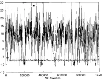
show the results from a regular canonical MC simula-tion at temperature T = 50 K (dotted curve) and those from a generalized-ensemble simulation of the new al-gorithm (solid curve). Here, the weight we used for the latter simulation is given by Eq. (17) with nF = 19 and E0 = EGS =
,12:2 kcal/mol. For the canon-ical run the curve stays around the value E = ,7 kcal/mol with small thermal uctuations, reecting the low-temperature nature. The run has apparently been trapped in a local minimum, since the mean energy at this temperature is < E >T=
,11:1 kcal/mol as found by a multicanonical simulation in Ref. [20]. On the other hand, the simulation based on the new weight covers a much wider energy range than the canonical run. It is a random walk in energy space, which keeps the simulation from getting trapped in a local mini-mum. It indeed visits the ground-state region several times in 1,000,000 MC sweeps. These properties are common features of generalized-ensemble methods.
Figure 1. Time series of the total energy E
tot (kcal/mol)
from a regular canonical simulation at temperatureT = 50
K (dotted curve) and that from a simulation of the present method with the parameters: E
0 =
,12:2 kcal/mol, n F =
19, and T= 50 K (solid curve).
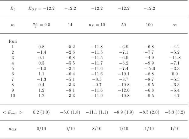
We now examine the dependence of the simulations on the values of the exponent m in our weight (see Eqs. (10) and (17)) and demonstrate that m = nF is indeed the optimal choice. Setting E0= EGS=
,12:2 kcal/mol,we performed 10 independent simulationruns of 50,000 MC sweeps with various choices of m. In Ta-ble 2 we list the lowest energies obtained during each of the 10 runs for ve choices of m values: 9:5 (= n
F 2 ), 14, 19 (= nF), 50, and 100. The results from regu-lar canonical simulations at T = 50 K with 50,000 MC
sweeps are also listed in the Table for comparison. If m is chosen to be too small (e.g., m = 9:5), then the weight follows a power law in which the suppression for higher energy region is insucient (see Eq. (13)). As a result, the simulations tend to stay at high energies and fail to sample low-energy congurations. On the other hand, for too large a value of m (e.g., m = 100), the weight is too close to the canonical weight, and there-fore the simulations will get trapped in local minima. It is clear from the Table that m = nF is the optimal choice. In this case the simulations found the ground-state congurations 80 % of the time (8 runs out of 10 runs). This should be compared with 90 % and 40 % for multicanonical annealing and simulated annealing algorithms, respectively, in simulations with the same number of MC sweeps [20].
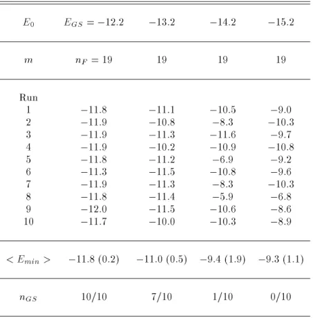
The weight factor of the present algorithm just de-pends on the knowledge of the global-minimum energy EGS (see Eq. (17)). If its value is known, which is the case for some systems, the weight is completely determined. However, if EGS is not known, we have to obtain its best estimate E0. In Table 3 we list the lowest energies obtained during each of 10 inde-pendent simulation runs of 200,000 MC sweeps with m = nF = 19. Four choices were considered for the E0 value:
,12:2; ,13:2; ,14:2, and ,15:2 kcal/mol. We remark that E0 has to underestimate EGS to en-sure that E,E
0 cannot become negative. Our data show that an accuracy of 1 2 kcal/mol in the es-timate of the global-minimum energy is required for Met-enkephalin.
Since the simulation by the present algorithm sam-ples a large range of energies (see Fig. 1), we can use the reweighting techniques [35] to construct canonical distributions and calculate thermodynamic quantities as a function of temperature over a wide temperature range.
which is calculated by a variant [42] of the double cu-bic lattice method [43]. Our denition of the overlap, which measures how much a given conformation diers from the ground state, is given by
O(t) = 1, 1 90n
F nF X i=1
j (t) i
, (GS) i
j; (26) where
(t) i and
(GS)
i (in degrees) stand for the n
F dihe-dral angles of the conformation att-th MC sweep and the ground-state conformation, respectively. Symme-tries for the side-chain angles were taken into account and the dierence
(t) i
, (GS)
i was always projected into the interval [,180
;180
]. Our denition guaran-tees that we have
0<O> T
1; (27)
with the limiting values
<O(t)> T
!1; T!0; <O(t)>
T
!0; T!1:
(28) We expect the folding of proteins and peptides to occur in a multi-stage process. A common scenario for folding may be that rst the polypeptide chain col-lapses from a random coil to a compact state. This coil-to-globular transition is characterized by the col-lapse transition temperature T
. In the second stage, a set of compact structures are explored. The nal stage involves a transition from one of the many local minima in the set of compact structures to the native (ground-state) conformation. This nal transition is characterized by the folding temperatureT
f ( T
). The rst process is connected with a collapse of the extended coil structure into an ensemble of compact structures. This transition should be connected with a pronounced change in the average potential energy as a function of temperature. At the transition temperature we therefore expect a peak in the specic heat. Both quantities are shown in Fig. 2. We clearly observe a steep decrease in total potential energy around 300 K and the corresponding peak in the specic heat dened by
C
1 N k
B d(<E
tot >
T) dT
= 2
<E 2 tot
> T
,<E tot
> 2 T N
; (29) where N (= 5) is the number of amino-acid residues in the peptide. In Fig. 3 we display the average values
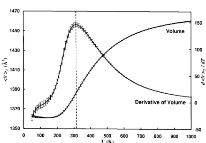
of each of the component terms of the potential energy (dened in Eq. (2)) as a function of temperature. As one can see in the Figure, the change in average po-tential energy is mainly caused by the Lennard-Jones term and therefore is connected to a decrease of the volume occupied by the peptide. This can be seen in Fig. 4, where we display the average volume as a func-tion of temperature. As expected, the volume decreases rapidly in the same temperature range as the potential energy.
Figure 2. Average total potential energy < Etot >T and
specic heat C as a function of temperature. The dotted vertical line is added to aid the eyes in locating the peak of specic heat. The results were obtained from a generalized-ensemble simulation of 1,000,000 MC sweeps.
Figure 4. Average volume < V >
T and its derivative d <V >T =dT as a function of temperature. The dotted
vertical line is added to aid the eyes in locating the peak of the derivative of volume. The results were obtained from a generalized-ensemble simulation of 1,000,000 MC sweeps.
If both energy and volume decrease are correlated, then the transition temperature Tcan be located both
from the position where the specic heat has its
maxi-mum and from the position of the maximaxi-mum of d < V >T
dT
2(< V E
tot>T ,< V >T< Etot>T) ; (30) which is also displayed in Fig. 4. The second quantity measures the steepness of the decrease in volume in the same way as the specic heat measures the steep-ness of decrease of potential energy. To quantify its value we divided our time series in 4 bins correspond-ing to 250,000 sweeps each, determined the position of the maximum for both quantities in each bin and aver-aged over the bins. In this way we found a transition temperature T= 28020 K from the location of the peak in specic heat and T = 31020 K from the maximum in d < V >T =dT. Both temperatures are
indeed consistent with each other within the error bars.
Table2. Lowest energy (in kcal/mol) obtained by the present method with several dierent choices of the exponent m. The case for m =1 stands for a regular canonical run at T = 50 K. < Emin > is the average of the lowest energy obtained by the 10 runs (with the standard deviations in parentheses), and nGS is the number of runs in
which a conformation with E,11:0 kcal/mol (the average energy at T = 50 K) was obtained.
E0 EGS=
,12:2 ,12:2 ,12:2 ,12:2 ,12:2
m nF
2 = 9:5 14 nF = 19 50 100
1 Run
1 0.8 ,5:2 ,11:8 ,6:9 ,6:8 ,4:2
2 ,1:4 ,2:6 ,11:5 ,7:1 ,7:7 ,5:2
3 0.1 ,6:8 ,11:5 ,6:9 ,4:9 ,11:8
4 0.5 ,5:5 ,11:7 ,8:2 ,9:9 ,7:1
5 ,1:0 ,3:4 ,11:6 ,7:4 ,12:0 ,3:3
6 1.1 ,6:4 ,11:6 ,10:1 ,8:8 0.9
7 ,1:3 ,5:1 ,8:5 ,8:7 ,8:7 ,5:3
8 0.4 ,3:3 ,9:7 ,10:8 ,9:5 ,6:3
9 1.2 ,8:1 ,11:6 ,12:0 ,6:8 ,6:4
10 1.2 ,3:3 ,11:9 ,10:8 ,9:5 ,4:7
< Emin> 0:2 (1:0) ,5:0 (1:8) ,11:1 (1:1) ,8:9 (1:9) ,8:5 (2:0) ,5:3 (3.2)
Table 3. Lowest energy (in kcal/mol) obtained by the present method with several dierent choices of the free parameter E0. < Emin> and nGS are the same as in Table 2.
E0 EGS=
,12:2 ,13:2 ,14:2 ,15:2
m nF = 19 19 19 19
Run
1 ,11:8 ,11:1 ,10:5 ,9:0
2 ,11:9 ,10:8 ,8:3 ,10:3
3 ,11:9 ,11:3 ,11:6 ,9:7
4 ,11:9 ,10:2 ,10:9 ,10:8
5 ,11:8 ,11:2 ,6:9 ,9:2
6 ,11:3 ,11:5 ,10:8 ,9:6
7 ,11:9 ,11:3 ,8:3 ,10:3
8 ,11:8 ,11:4 ,5:9 ,6:8
9 ,12:0 ,11:5 ,10:6 ,8:6
10 ,11:7 ,10:0 ,10:3 ,8:9
< Emin> ,11:8 (0:2) ,11:0 (0:5) ,9:4 (1:9) ,9:3 (1:1)
nGS 10/10 7/10 1/10 0/10
Figure 5. Average overlap < O >T and its derivative d <O >
T
=dT as a function of temperature. The dotted
vertical line is added to aid the eyes in locating the peak of the derivative of overlap. The results were obtained from a generalized-ensemble simulation of 1,000,000 MC sweeps.
The second transition which should occur at a lower temperature Tfis that from a set of compact structures
to the \native conformation" that is considered to be the ground state of the peptide. Since these compact conformations are expected to be all of similar volume and energy, we do not expect to see this transition by
pronounced changes in < Etot >T or to nd another
peak in the specic heat. Instead this transition should be characterized by a rapid change in the average over-lap < O >T with the ground-state conformation (see
Eq. (26)) and a corresponding maximum in d < O >T
dT
2(< OE
tot>T ,< O >T< Etot>T) : (31) Both quantities are displayed in Fig. 5, and we indeed nd the expected behavior. The change in the order parameter is clearly visible and occurs at a tempera-ture lower than the rst transition temperatempera-ture T. We
again try to determine its value by searching for the peak in d < O >T =dT in each of the 4 bins and
av-eraging over the obtained values. In this way we nd a transition temperature of Tf = 23030 K. We re-mark that the average overlap < O >T approaches its
limiting value zero only very slowly as the temperature increases. This is because < O >T = 0 corresponds
steric hindrance of both main and side chains.
We remark that the above algorithm was also suc-cesfully applied to a more direct evaluation of the free-energy landscape of small peptides [44], which allowed us to visualize the folding funnel of the molecule.
IV. Conclusions
In this article we have reviewed the uses of Tsal-lis statistical mechanics in the protein folding prob-lem. Monte Carlo simulated annealing algorithm and generalized-ensemble algorithm with both Monte Carlo and stochastic dynamics algorithms were introduced. A penta peptide, Met-enkephalin was used to study the performances of these algorithms. While other generalized-ensemble algorithms suer from the di-culty that the determination of the optimal weight fac-tor is non-trivial and tedious, it was shown that its determination in the Tsallis generalized-ensemble algo-rithm is much simpler than other versions.
Acknowledgements
:Our simulations were performed on the computers of the Computer Center at the Institute for Molecular Science, Okazaki, Japan. This work is supported, in part, by a Grant-in-Aid for Scientic Research from the Japanese Ministry of Education, Science, Sports and Culture, by a grant from the Research for the Future Program of Japan Society for the Promotion of Science (JSPS-RFTF98P01101) and by a Research Excellence Fund (E27448) of the State of Michigan.
References
[1] S. Kirkpatrick, C.D. Gelatt, Jr., and M.P. Vecchi,
Science220, 671 (1983).
[2] B.A. Berg and T. Neuhaus, Phys. Lett.B267, 249
(1991);Phys. Rev. Lett.68, 9 (1992).
[3] B.A. Berg,Int. J. Mod. Phys.C3, 1083 (1992).
[4] U.H.E. Hansmann and Y. Okamoto,J. Comp. Chem.
14, 1333 (1993).
[5] A.P. Lyubartsev, A.A.Martinovski, S.V. Shevkunov, and P.N. Vorontsov-Velyaminov,J. Chem. Phys.96,
1776 (1992).
[6] E. Marinari and G. Parisi, Europhys. Lett. 19, 451
(1992).
[7] B. Hesselbo and R.B. Stinchcombe,Phys. Rev. Lett.
74, 2151 (1995).
[8] U.H.E. Hansmann and Y. Okamoto,J. Comp.Chem.
18, 920 (1997).
[9] U.H.E. Hansmann, Y. Okamoto and F. Eisenmenger,
Chem. Phys. Lett.259, 321 (1996).
[10] N. Nakajima, H. Nakamura and A. Kidera,J. Phys. Chem.101, 817 (1997).
[11] C. Bartels and M. Karplus, J. Phys. Chem. B102,
865 (1998).
[12] C. Tsallis, J. Stat. Phys.52, 479 (1988).
[13] U.H.E. Hansmann and Y. Okamoto,Phys. Rev. E56,
2228 (1997).
[14] U.H.E. Hansmann, F. Eisenmenger, and Y. Okamoto,
Chem. Phys. Lett.297, 374 (1998).
[15] F.A. Momany, R.F. McGuire, A.W. Burgess, and H.A. Scheraga, J. Phys. Chem.79, 2361 (1975); G.
Nemethy, M.S. Pottle, and H.A. Scheraga, J. Phys. Chem.87, 1883 (1983); M.J. Sippl, G. Nemethy, and
H.A. Scheraga,J. Phys. Chem.88, 6231 (1984).
[16] H. Kawai, Y. Okamoto, M. Fukugita, T. Nakazawa, and T. Kikuchi, Chem. Lett. 1991, 213 (1991); Y.
Okamoto, M. Fukugita, T. Nakazawa, and H. Kawai,
Protein Eng.4, 639 (1991).
[17] The program SMC was written by F. Eisenmenger. [18] N. Metropolis, A.W. Rosenbluth, M.N. Rosenbluth,
A.H. Teller, and E. Teller, J. Chem. Phys.21, 1087
(1953).
[19] S. Geman and D. Geman, IEEE Trans. Patt Anal. Mach. Intel6, 721 (1984).
[20] U.H.E. Hansmann and Y. Okamoto, J. Phys. Soc. Jpn.63, 3945 (1994);Physica A212, 415 (1994).
[21] S.R. Wilson, W. Cui, J.W. Moskowitz, and K.E. Schmidt,Tetrahedron Lett.29, 4373 (1988).
[22] H. Kawai, T. Kikuchi, and Y. Okamoto,Protein Eng.
3, 85 (1989).
[23] C. Wilson and S. Doniach,Proteins6, 193 (1989).
[24] A.T. Brunger,J. Mol. Biol.203, 803 (1988).
[25] M. Nilges, G.M. Clore, and A.M. Gronenborn,FEBS Lett.229, 317 (1988).
[26] M. Pellegrini, N. Grnbech-Jensen, and S. Doniach,
Physica A239, 244 (1997).
[27] M. Kinoshita, Y. Okamoto, F. Hirata,
J. Am. Chem. Soc.120, 1855 (1998).
[28] L. Carlacci,J. Comp-Aided Mol. Des.12, 195 (1998).
[29] Y. Okamoto, M. Masuya, M. Nabeshima and T. Nakazawa,Chem. Phys. Lett.299, 17 (1999).
[30] H. Szu and R. Hartley,Phys. Lett.A122, 157 (1987).
[31] D.A. Stariolo and C. Tsallis, in Annual Reviews of Computational Physics II, edited by D. Stauer (World Scientic, Singapore, 1995), p. 343.
[32] T.J.P. Penna,Phys. Rev. E51, R1 (1995).
[33] I. Andricioaei and J.E.Straub, Phys. Rev. E 53,
R3055 (1996).
[35] A.M. Ferrenberg and R.H. Swendsen, Phys. Rev. Lett.61, 2635 (1988);ibid.63, 1658(E) (1989).
[36] D.A. Stariolo,Phys. Lett.A185, 262 (1994).
[37] I. Andricioaei and J.E. Straub,J. Chem. Phys.107,
9117 (1997).
[38] G. Parisi and Y.-S. Wu,Sci. Sin.24, 483 (1981).
[39] S. Duane, A.D. Kennedy, B.J. Pendleton, and D. Roweth, Phys. Lett. B195, 216 (1987). references
given in the erratum.
[40] Y. Okamoto, T. Kikuchi, and H. Kawai,Chem. Lett.
1992, 1275 (1992).
[41] U.H.E. Hansmann, M. Masuya, and Y. Okamoto,
Proc. Natl. Acad. Sci. USA94, 10652 (1997).
[42] M. Masuya, in preparation.
[43] F. Eisenhaber, P. Lijnzaad, P. Argos, C. Sander, and M. Scharf,J. Comp. Chem.16, 273 (1995).