Bearing Health Monitoring

Tribology in Industry

www.tribology.fink.rs

Bearing Health Monitoring

S. Shah

_{, A. Guha}

a_{Department of Mechanical Engineering, IIT Bombay, Powai, Mumbai 400076, India.}

Keywords:

Bearing health monitoring Vibration

Kurtosis

Empirical mode decomposition Intrinsic mode function

A B S T R A C T

Health monitoring of bearings is a widely researched topic and has been attempted by analysing acoustic, thermal and vibration signatures. The methods usually require signal of a healthy bearing to be used as a baseline. This limits their use in practical scenarios. This work proposes a kurtosis based baseline free method of analysing vibration signals to identify the bearing which has generated a fault. It then reports a detailed study on empirical mode decomposition technique for extracting intrinsic mode functions and suggests a set of steps which are necessary and sufficient for the purpose of bearing health monitoring. Thereafter, it compares a few dominant frequencies with the expected ones based on known bearing dimensions. This process has been shown to be fairly accurate in identifying the location of fault in a bearing.

© 2016 Published by Faculty of Engineering Corresponding author:

Anirban Guha

Department of Mechanical Engineering, IIT Bombay, Powai, Mumbai 400076, India.

E-mail: anirbanguha1@gmail.com

1. INTRODUCTION

Bearing health monitoring can have three components - detection of anomalous bearing behaviour, identification of the specific component of the bearing which is defective or has undergone unacceptable degradation and prediction of remaining life. Tandon et al [1] have reviewed various methods for bearing health monitoring. Acoustic, temperature and vibration measurements are some of the widely used methods. All of them have their own advantages and disadvantages. Testing the lubricant for debris has been shown to be a reliable method of identifying the type of fault (i.e. the specific region of the bearing causing the anomaly). The choice of lubricating oil in important in this context [15]. However, the off-line and periodic nature of this method of detection led us to investigate other methods of

fault type (zone) identification. Continuous monitoring is possible with vibration signals if a reliable method of filtering and analysing the signal can be decided upon. This is what has been attempted in this work.

Identification of the specific component of the bearing which has developed a fault by analysing the vibration signal requires some prior knowledge about the type of bearing. For roller bearings, the defect can be on the inner race, outer race or the rollers. Each of these generates a characteristic pulse of a specific frequency which depends on the dimensions of the different components of the bearing. Lacey [2] has discussed this and has given additional defect frequencies comprising of the harmonics for each of the three defects. Huang et al [3]

have shown how Empirical Mode

Decomposition (EMD) can be used to

R

E

S

E

A

R

C

decompose a signal into its components. The signal obtained from a bearing usually contains significant noise which needs to be filtered out. Lei et al [4] show how such de-noising can be done using Ensemble Empirical Mode Decomposition (EEMD). The use of EMD requires a number of parameters of the analysis to be fine tuned as reported in the work of Nikolakopoulos and Zavos [16]. Some of these aspects, e.g. the stoppage criteria, have been investigated by Rilling et al [3] and Huang et al [5]. However, a necessary and sufficient set of procedures needed to extract useful information from bearing vibration data is yet to be reported.

A completely different approach - use of Self Organising Maps - has been explored by Qiu et al [6]. They have used data generated by NSF I/UCRC Centre for Intelligent Maintenance Systems for analysis and have attempted to assess the state of degradation of bearings. Wavelets have also been used to identify presence of fault and a review of papers on this topic is given by Kumar et al [7]. However, the advantage of using EMD over wavelet decomposition or fourier transform for analyzing real life signals which can arise from multiple reasons is also well documented [12-13]. Yu [8] has applied unsupervised machine learning on the NSF data and has attempted to predict the presence of bearing fault. Xue et al [9] have used auto-correlation followed by Intrinsic Mode Function (IMF) extraction using EMD and feature extraction to identify the type of fault. Noise was found to be a hindrance in this procedure. The machine learning methods are promising. However, their efficacy needs to be compared with the other methods before they can be established as a viable alternative. This has not been reported so far.

In this paper, we have identified a simple statistical measure which can indicate the presence or absence of a fault. The fact that this is a baseline free method (not requiring past or fault free data) makes it attractive for application in real life conditions. We have also arrived at a sequence of steps for EMD which gives the best method of extraction of frequencies of defects. This helps in identifying the types of the defects based on data mentioned by Lacey [2].

2. DATA SET

The data set used for this work was obtained from a NASA Date Repository [10]. Figure 1 shows the test bed. The set up consists of four bearings, thus generating four sets of data. Rexnord ZA- 2115 double row bearing was used. Readings were taken using PCB 353B33 High Sensitivity Quartz ICP accelerometers. Frequency of reading was 20 kHz and readings were taken for 1.024 seconds, thus giving 20480 points in each reading.

Fig. 1. Bearing test rig and sensor placement [6].

Table 1. Data set summary [4]. Duration of

test

Number of files

(points) Defect Description 22/10/2003

25/11/2003

2156 (2156*20480)

Inner race defect–bearings 3 Roller element defect–bearings 4

Table 1 gives the summary of test and the bearings which failed at the end of test. It may be noted that only the type of fault at end of test was reported and not the degree of degradation.

3. DETECTING PRESENCE OF FAULT

Fig. 2. (a) Signal of healthy bearing, (b) signal of defective bearing.

Fig. 3. Kurtosis plot of Test 1 Data.

One way to characterise the peaks of such signals is by kurtosis. In Fig. 3, y axis is the kurtosis of one instance of reading (20480 points in our case) and x-axis is the reading number, which is also representative of time. The test consisted of 2156 files, of which we have considered equally spaced 350 files (spread over three days) for our analysis. It can be seen that development of fault is accompanied by a sharp rise in kurtosis for bearings 3 and 4.

We can see that this simple method is effective in detecting the presence of fault in bearing. We also propose that a kurtosis of 6 may be taken as the threshold. A significant number of readings with a

kurtosis above 6 can be taken as an indicator of a bearing having developed a fault. The advantage of this method is that it does not require any past data or history of bearing readings.

4. EMPIRICAL MODE DECOMPOSITION

This section will give a brief description of EMD which will be used to determine the type (location) of fault. EMD allows the signal to be decomposed into Intrinsic Mode Functions (IMFs) based on the time characteristic of signal. The algorithm is:

1. Let the given data be xmain 2. x=xmain

(a) (b)

3. Calculate the maxima and minima of the x 4. Draw a spline through the maxima and a

separate spline through the minima 5. Calculate the mean: mean =(maxima

spline + minima spline)/2

6. Subtract this mean from the signal x and get a new x as x=x-mean

7. Repeat processes 3 to 6 till we get an IMF. The signal at end of step 6, after a number of iterations, is the first IMF. 8. Subtract the first IMF from the original

data: xmain=xmain - IMF and go back to step 2 and use this as new data to get the second IMF.

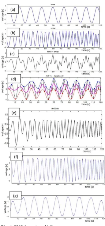
The first IMF will have the highest frequency, the second IMF will have the second highest frequency and so on. Figure 4 shows the various steps of a typical example. Figures 4(a) and 4(b) show tone and chirp which have been combined into a single signal in 4(c). This combined signal is the input to our analyser and on performing EMD we get two IMFs 4(f) and 4(g), which are the tone and chirp. Figure 4(d) shows one iteration where we have plotted the spline for maxima and minima and their mean. The blue curve is a spline through the maxima, the orange curve is a spline through the minima and the pink curve is the mean of these two splines. Figure 4(e) displays the residue left after subtracting the mean from the signal. This is same as step 6 in the above algorithm. This procedure is repeated several times to get the IMFs.

4.1 De-Noising [4]

Every real life signal contains some noise which needs to be filtered out. Ensemble Empirical Mode Decomposition (EEMD) is one method of achieving this. In this we add white Gaussian noise to the signal and then extract the IMF. Then we again add white Gaussian noise to the original signal and repeat the same procedure. White noise is generated randomly and so it is different every time. So, the two IMFs differ a little from each other. The average of the two IMFs is a better indicator of the constituent signal than the IMF extracted without adding the white Gaussian noise. Instead of two, we can take 50 or 100 such IMFs and average them out. This has been shown to be an effective procedure for de-noising the signal.

Fig. 4. EMD Iterations [14].

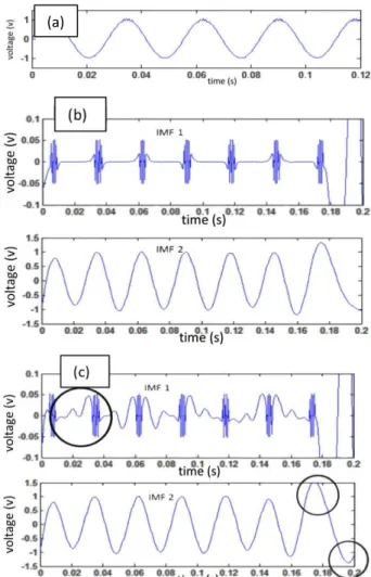
Fig. 5. (a) Sine wave with noise, (b) EEMD with average of 100, (c) EMD.

The efficacy of EEMD comes at a cost of extra computing effort. Thus, a decision needs to be taken on whether or not to prefer it over EMD and if so, how many instances of white noise addition needs to be done. This would be dependent on the specific application and a study was conducted to ascertain this for the current study on bearing vibration signals. Both EMD and EEMD were applied on the bearing data. The difference in results was not found to be significant enough to justify EEMD. Thus, the rest of the work used EMD rather than EEMD.

4.2 Curve Fitting

A critical decision in EMD is the choice of the curve which needs to pass through the maxima and minima of the signal. This is usually a spline. However, improper selection of end conditions can lead to overshooting and undershooting. The usual technique of averaging the maxima (or minima) near the end may not be effective as shown in Fig. 6. In both Figs. 6 and 7, the blue

curve is the original signal and the red curve is a spline drawn through the maxima. The problem of excessive undulation between two points (maxima or minima) may remain even with proper end conditions as seen in Fig. 6(a). Piecewise cubic hermitian interpolation [11] was found to give the best result (Fig. 7) and was adopted for the rest of the work.

4.3 Stoppage Criteria

IMF extraction involves repeated subtraction of the mean of the maxima and minima splines from the signal, as explained in a previous section. Repeated iterations result in a better (more accurate) IMF. However, this comes at the cost of computational effort and time. An effort was made in this work to determine the appropriate criterion to stop the iterations. Huang

et al s [ ] method is based on the difference in

deviation (as defined in equation 1) between IMFs extracted in two successive iterations. A low difference indicates time to stop.



 



















t n

n n

t

h

t

h

t

h

Deviation

0

2 1

2 1

)

(

|

)

(

)

(

|

(1)

where: T= Total time of reading, hn-1(t) = residue

obtained after n-1 iterations, hn(t) = residue

obtained after n iterations.

Fig. 6. (a) Spline interpolation with end conditions specified (b) Spline interpolation with no end conditions.

Fig. 7. Piecewise Cubic Hermitian Interpolation.

It was found that a difference of 0.2 to 0.3 between successive deviations is a reasonable stoppage criterion.

Another criterion explored was a point by point comparison of the IMFs extracted in successive iterations and stopping when the difference becomes less than 10 % of maximum. It was found that this difference does not always show a monotonically decreasing trend. Thus, two sub-criteria were explored – the difference being less than 10 % for the first time and the difference being less than 10 % for a significant number of iterations. The latter gave better results.

The results obtained by these refined stoppage criteria were compared with those obtained by a simple criterion, namely a fixed number of iterations as suggested by Rilling et al [5]. The latter was found to give results quite comparable to those of the earlier methods at a much lower processing time. Our data allowed good IMF extraction at 8 iterations whereas the earlier methods required 50 to 100. Thus, the criterion of using a fixed number of iterations for IMF extraction was recommended and used for the rest of this work.

5. DEFECT IDENTIFICATION

The formulae for fundamental defect frequency for roller bearings where inner race rotates have been given in equations 2, 3 and 4 [1].

Outer race defect frequency

      

 1 cos



2 D d d zf f s od (2)

Inner race defect frequency











 



1

cos



2

D

d

d

zf

f

Rolling element defect frequency



















2 2

cos

1

2

D

d

d

zf

f

where, fs= speed of shaft rotation in Hz

z=number of rolling elements D=pitch diameter

d=roller diameter

α=contact angle

Additional fault frequencies based on harmonics as given by Lacey [2] are listed below in Table 2.

Table 2. Bearing Defect Frequencies [2].

Surface Defect

Frequency

Component Imperfection

Inner Raceway

Eccentricity

f

Waviness

nZf



f

Discrete Defect

nZf



f

Outer Raceway

Waviness

nZf

Discrete Defect co s

f nZf  co co f nZf  Roller Element

Diameter Variation Zf_co

Waviness

2

nf



f

Discrete Defect

2

nf



f

where, fs = speed of rotation

Z = number of rolling elements n = index starting from 0

      

 1 cos



2 1 D d d f_co       

 1 cos



2 1 D d d f_ci



















2 2

cos

1

2

1

D

d

d

f

Table 3 shows the dimensions of bearing ZA-2115 used for this study and associated fault frequencies as obtained from these formulae.

Table 3. ZA-2115 bearing dimensions and defect frequencies.

Quantity Value

Pitch Diameter 71.5 mm

Diameter of Rollers 8.4 mm

Number of Rolling Elements 16

Contact Angle 15.17o

Rotating Frequency 33.333 Hz

Outer race defect frequency ( fod) 236.43 Hz

Inner race defect frequency ( fid ) 297 Hz

Rolling element defect frequency ( fre ) 280 Hz

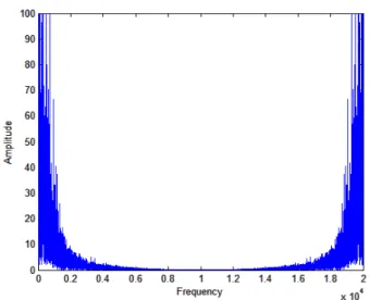
Figure 8 is the plot of FFT of IMF 1 of a certain bearing which has already developed a fault. In Table 4 we have also listed the top 10 dominant frequencies. We can see that the plot is dominated by high frequencies which are not relevant to our investigation. Many options were attempted to get rid the FFT plot of the unnecessary high frequencies. The one which showed the best result was squaring of the IMF and then taking its FFT.

Fig. 8. Plot of FFT of IMF 1 of a faulty bearing.

Table 4. Dominant frequencies in plot 8.

Dominant Frequencies

4022.5

4182.6

3949.2

4024.4

4174.8

3949.2

4037.1

3963.9

4039.1

3978.5

Figure 9 shows the corresponding plot and the dominant frequencies are shown in Table 5. The high frequencies have clearly been suppressed and the frequencies in our range of interest are now available. We see the presence of frequency around 232 Hz and 280 Hz, denoting that there is a fault in the bearing which is actually the case.

Fig. 9. Plot of FFT of square of IMF 1 of a faulty bearing.

Table 5. Dominant frequencies in plot 9.

Dominant Frequencies

0

14.65

465.82

261.72

276.37

232.42

72.27

698.24

73.24

464.84

Fig. 10. Plot of FFT of smoothen IMF 1 of a faulty bearing.

Table 6. Dominant frequencies in plot 10.

Dominant Frequencies

0

14.65

465.82

232.42

261.72

464.84

276.37

698.24

33.203

72. 27

The previous sections have described the large number of options available while implementing EMD. Through a systematic study it was possible to arrive at a combination of these options which is reasonable and practical for bearing health monitoring. The ensuing section will describe how this was applied to the data set of Table 1.

6. APPLICATION OF EMD

Out of the 2156 files (Table 1), 350 were chosen such that the data pertained to readings taken at approximately 1 hour intervals. The EMD procedure described in the previous sections was implemented. The IMFs were smoothened and the dominant frequencies were detected.

In Figures 11 to 13, x-axis indicates reading number and y-axis shows the number of fault frequencies present in the first 10 dominant frequencies of the IMF. Figure 11 shows plots in which we compare the top 10 dominant frequencies present in the IMF with frequencies obtained in equations 2 to 4. If a particular frequency is present then we get +1 for the reading, if two frequencies match then we get +2 and so on. This is done for both IMF 1 and IMF 2.

Fig. 12. Results of Test 1 based on Table 2.

Fig. 13. Results of Test 1 without extracting IMF and based on Table 2.

Figure 12 shows the results when the 10 dominant frequencies are compared with frequencies obtained by equations given in Table 2.

In Figure 11, the plots for bearings 1 and 2 show low values indicating that the dominant

reported to have a roller element fault and this too can be concluded. However, the plots also indicate the presence of inner and outer race faults for bearing 4.

This has not been reported in the information available about the test. This leads to the tentative conclusion that inner and outer race faults can be definitively identified by the procedure suggested in this paper. However, if roller element faults are present, they can be identified, but may give rise to false positive signals for inner and outer race faults.

Figure 12 was generated by comparing the 10 dominant frequencies with the frequencies obtained by the equations of Table 2. This was done with the expectation that comparison with the higher harmonics would lead to easier differentiation between cases of high and low number of matches. Unfortunately, this did not turn out to be true. Figure 12 show that an attempt to include higher harmonics in this analysis leads to an obfuscation of the difference between data with and without faults.

Figure 13 shows an attempt to repeat the analysis by using the original signal and not the IMFs. This is shown to be a failure, thus establishing the need for IMF extraction through EMD as a prerequisite before extracting the dominant frequencies through FFT.

7. CONCLUSION

This paper attempts to establish a method of analysing vibration signals of bearings for their health monitoring. Out of the three primary tasks in this exercise, namely, identification of the bearing which has a fault, detection of the region of the bearing which has developed a fault and prediction of the remaining useful life of a bearing, this paper attempts the first two. Identification of the bearing which has developed a fault has been shown to be possible by a kurtosis plot - a value higher than 6 indicating the presence of a fault. The baseline free nature of this parameter makes it easily applicable to practical situations where data for a completely undamaged bearing may not be available.

Detection of the region of the bearing which has developed a fault requires extraction of IMFs

from the signal with EMD. This paper explores the large number of options available at various stages of EMD and suggests a set of options which are necessary and sufficient from the point of view of bearing health monitoring. A method of comparing the first 10 dominant frequencies with the expected frequencies led to a clear identification of the faults along with a possibility of false positive signals in the presence of a fault in the rolling element.

REFERENCES

[1] N. Tandon and A. Choudhury, A review of vibration and acoustic measurement methods for the detection of defects in rolling element

bearings , Tribology International, vol. 32, pp. 469-480, 1999.

[2] S. J. Lacey, An overview of bearing vibration

analysis , Maintenance and Asset Management, vol. 23, no. 6, 2008.

[3] N. E. Huang, Z. Shen, S. R. Long, M. C. Wu, H. H. Shih, Q. Zheng, N. C. Yen, C. C. Tung and H. H. Liu, The empirical mode decomposition and the Hilbert spectrum for nonlinear and

non-stationary time series analysis , Proceedings of the Royal Society A: Mathematical, Physical and Engineering Sciences, vol. 454, pp. 903-995, 1998.

[4] Y. Lei, Z. He and Y. Zi, EEMD method and WNN

for fault diagnosis of locomotive bearings

Expert Systems with Applications, vol. 38, no. 6, pp. 7334-7341, 2011.

[5] G. Rilling, P. Flandrin and P. Goncalves, On empirical mode decomposition and its

algorithms , in Proceedings of IEEE-EURASIP Workshop on Nonlinear Signal and Image Processing NSIP-03, Grado (Italy), June 2003. [6] H. Qiu, J. Lee, J. Lin and G. Yu, 006. Wavelet

filter-based weak signature detection method and its application on roller bearing

prognostics ,Journal of Sound and Vibration, vol. 289, pp. 1066-1090, 2006.

[7] H. S. Kumar, S. P. Pai, G. S. Vijay and R. B. K. N.

Rao, Wavelet transform for bearing condition monitoring and fault diagnosis: A review, International Journal of COMADEM, vol. 17, no. 1, pp. 9-23, 2014.

[8] J. Yu, Health condition monitoring of machines based on hidden Markov model and

[9] Y. J. Xue, J. X. Cao, R. F. Tian and Q. Ge, Feature extraction of bearing vibration signals using autocorrelation denoising and improved Hilbert-Huang transformation International Journal of Digital Content Technology and its Applications, vol. 6, no. 4, pp. 150-158, 2012. [10] NASA Data Repository, available at

http://ti.arc.nasa.gov/tech/dash/pcoe/prognos tic-data-repository/, accessed: 17.07.2015. [11] W. Zhu, H. Zhao and C. Xiaoping, Improving

empirical mode decomposition with an optimized piecewise cubic Hermite

interpolation method in International Conference on Systems and Informatics (ICSAI), Yantai, China, 2012.

[12] Empirical Mode Decomposition, available at https://www.clear.rice.edu/elec301/Projects02 /empiricalMode/, accessed: 11.08.2015.

[13] L. Lin, Y. Wang and H. Zhou, 009. Iterative filtering as an alternative algorithm for

empirical mode decomposition , Advances in Adaptive Data Analysis, vol. 1, no. 4, pp. 543-560, 2009.

[14] EMD, available at http://perso.ens-lyon.fr/patrick.flandrin/emd.ppt, accessed: 12.08.2015.

[15] R. Rakic, The choice of lubricating oil for rolling

bearings of machine tools , Tribology in Industry, vol. 19, no. 3, pp. 113-116, 1997.