A 22-year cycle in the F layer ionization of the ionosphere
E. Feichter, R. Leitinger
Institut fuÈr Meteorologie und Geophysik, UniversitaÈt Graz, HalbaÈrthgasse 1, A-8010 Graz, Austria Tel: +43 316 380 5257; Fax: +43 316 384091; e-mail: [email protected]
Abstract. The double-sunspot-cycle variation in terres-trial magnetic activity has been well known for about 30 years. In 1990 we examined and compared the low-solar-activity (LSA) part of two consecutive cycles and predicted from this database and from published results the existence of a double-sunspot-cycle variation in total electron content (TEC) of the ionosphere too. This is restricted to noontime when the semi-annual component is well developed. Since 1995 we have had enough data for the statistical processing for high-solar-activity (HSA) conditions of two successive solar cycles. The results con®rm the LSA ®ndings. The annual variation of TEC shows a change from an autumn maximum in cycle 21 to a spring maximum during the next solar cycle. Similar to theaa indices for geomagnetic activity the TEC data show a phase change in the 1-year component of the Fourier transform of the annual variation. Additionally we found the same behaviour in the F-layer peak electron density (Nmax) over four solar cycles. This indicates that there exists a double-sunspot-cycle variation in the F-layer ionization over Europe too. It is very likely coupled with the 22-year cycle in geomagnetic activity.
1 Introduction
The main data source for the work on which this report is based was provided by the dierential Doppler eect on the signals of the US Navy Navigation Satellites (NNSS, formerly TRANSIT, in almost polar circular orbits with a height around 1100 km) (Leitinger et al., 1975; Leitinger and Putz, 1978).
Two European receiving stations have been in continuous coordinated operation since the beginning
of 1975: Lindau/Harz in Germany (51:6N, 10:1E) and
Graz in Austria (47:1N, 15:5E). The evaluation results
are latitudinal pro®les of ionospheric electron content, which means sequences of data equidistant in latitude (data distance 0:5in geographic latitude of the 400-km
ionospheric points). Up to the mid-1980s the observa-tions from Lindau gave more material and were used for the statistical investigation for the interval 1975±1986. The data of the station Graz were applied indirectly, namely to calibrate electron content by means of the ``two-stations method'' (Leitinger et al., 1975). For the high-solar-activity interval of 1988±92 the observations from Graz were used. For a given latitude there is no signi®cant dierence in monthly medians and quartiles calculated from Graz and Linda data.
For this report the electron-content values for the geographical latitudes 60N, 55N, 50N and 45N were selected. The data from Graz which reach 30N show that the results are valid down to 35N, where the in¯uence of the equatorial anomaly begins at HSA conditions.
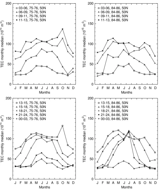
The total electron content (TEC) data used for this study are monthly medians gained over 2-h intervals. The data were divided into two classes: low solar activity (LSA) (R40; nominal monthly mean sunspot number for modelling purposes: R20) and high solar activity (HSA) [130R170 (cycle 21), 120R180 (cycle 22), respectively, nominal valueR150]. (The widening of the R interval for HSA/cycle 22 was necessary in order to ensure data from at least 2 years for each month. Using data according to the criterion 130
R12170 ± all months from November 1988 to
December 1991 ± leads to nearly identical results in statistical investigations.)
The amount of TEC data from intermediate levels of solar activity (MSA) is not sucient to make clear statements about the ionization behaviour under these conditions. The results of investigations of peak electron density (Nmax) show that there is no substantial dier-ence between the annual variation for MSA and HSA.
These selection criteria enabled us to include all data from the years 1975 and 1976 and the data from July
1984 to December 1986 into the LSA class and data from 1978±1982 selected according to Table 1 and from 1988±1992 selected according to Table 2 into the HSA class. The comparatively large variation in HSA-Rmight be a problem, especially when seasonal dierences are to be investigated. The month-to-month dierences in R are cancelled out at least partially in averages: the cycle 21 vernal average (March 1979, 1982; April 1980, 1981) is R153, the autumnal one (September, 1978, 1981; October 1980, 1981) R158; the cycle-22 vernal aver-age (March and April 1989, 1990, 1991) isR137, the autumnal one (September and October 1988, 1989, 1990, 1991)R140. Both for monthly medians of TEC and ofNmax(or foF2) one ®nds considerable dierences comparing data gained under comparable seasonal and solar activity (R;R12 or any other solar index)
condi-tions. Therefore some averaging is necessary. In the TEC case this was done by selecting the observed data into (129, cycle-21, or 1212 months, cycle 22) classes (the 12 months of the year and 9 or 12 LT intervals). Medians were calculated for each data class. The ®rst statistical studies (see Feichter et al., 1988, 1990, 1991; Feichter and Leitinger, 1993) could be based on two LSA intervals (1975±1976 and 1984±1986) (Fig. 1) and on the cycle-21 HSA interval (1978±1982). In 1989 we investigated data of 1984±1986 to be able to compare two consecutive solar minima (1975±1976 and 1984±1986) (Feichter et al., 1990). Since 1995 we have had enough data to compare the HSA period of cycle 22 (selected months 1988 to 1992, see Table 2) with that of cycle 21 too.
To extend the investigation to a wider range of solar cycles we obtained the annual variation of Nmax with ionosonde scalings (hourly values of foF2) from several ionosonde stations (Table 3). ForNmaxlinear regressions
were applied to ®nd the relation between solar activity (R12) and peak electron density for each month and for
each hour of the day. From the linear regression relation Nmaxwas calculated for a selected level of solar activity. The regressions were based on dierent data selections, e.g. all data of one solar cycle, data from the rising part of a cycle and data from the falling part, the interval around the solar maximum. Some regressions failed and gave negative slopes and/or negative R120
intercep-tion points. However, no failures occurred during daytime. For HSA (R12150) and intermediate levels
of solar activity (e.g.R1285) the 22-year periodicity is
stable and does not depend on the data selection for the regressions: it appears when all data of one cycle are included, and in partial data (rising part, falling part, etc.). The examples used in this report show HSA (R12150) cases of one ionosonde station, Rome, Italy
(41:8N, 12:5E).
An additional remark: attempts to ®nd a solar-cycle dependence in tropospheric dynamics (``weather'') have been based on the cycle-to-cycle dierences of the semi-annual component of magnetic activity (Baranyi and LudmaÂny, 1992, 1995a, 1995b). An in¯uence on the ionosphere is much more likely than an in¯uence on the troposphere
2 Data Analysis
The results are discussed in terms of the Fourier transform of the twelve monthly medians of the annual variation (cosine termsa0 a6, sine termsb1 b5) and
reconstruction to ordern:
Fn t
X
n
j0
ajcos jxt
X
n
j1
bjsin jxt
a0a1cos xt b1sin xt a2cos 2xt
b2sin 2xt
C0C1cos xtÿ/1 C2cos 2xtÿ/2
with Cj
a2
jb2j
q
and tan/j bj aj
:
x2p
12 tin months or x 2p
365:25 tin days
Table 1.Monthly mean sunspot numbersRfor the solar maximum
period 1978±1982 [<:R<130 (not selected), >:R>170 (not selected), x: no data available]
HSA (solar cycle 21)
J F M A M J J A S O N D
1978 < < < < < < < < 138 < < < 1979 167 138 138 < 134 150 159 142 > > > > 1980 160 155 < 164 > x 136 135 x 165 148 > 1981 < x x 156 < < 144 159 167 162 138 150 1982 < 164 154 < < < < < < < < <
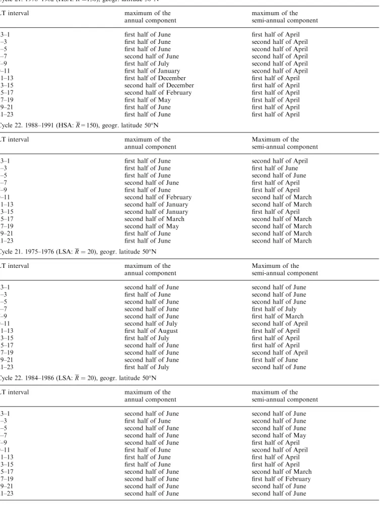
Table 2.Monthly mean sunspot numbersRfor the cycle-22 solar
maximum period 1988±1992 [<:R<120 (not selected),>:R>180 (not selected)]
HSA (solar cycle 22)
J F M A M J J A S O N D
1988 < < < < < < < < 120 125 125 179 1989 161 165 131 131 139 > 127 169 177 159 173 166 1990 177 131 140 140 132 < 149 > 125 146 131 130 1991 137 168 142 140 121 170 174 176 125 144 < 141 1992 150 161 < < < < < < < < < <
Table 3. Data sources for the ®gures with F-layer ionization
examples solar cycle
years data and sources method
The Fourier decomposition gives the possibility to study asymmetries in the annual variation by means of the relation of the 1-year component to the 1/2-year component.
2.1 Behaviour of the amplitudes
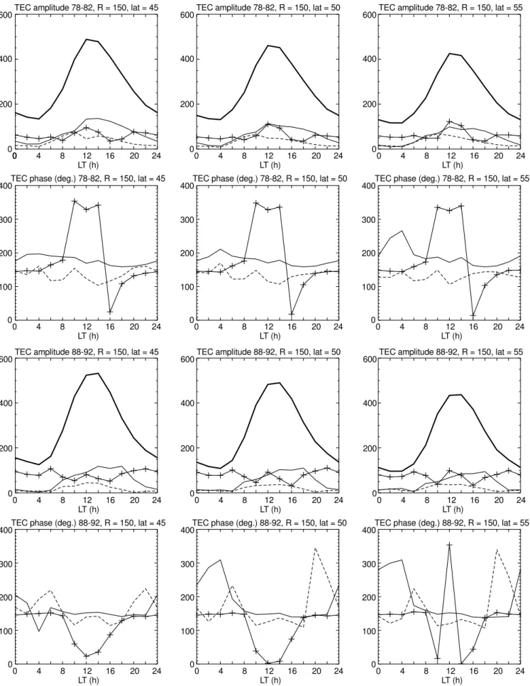
The average values (C0a0) increase with decreasing
latitude. From solar cycle to solar cycle the change in value of the maximum of the average is less than 10%. The general level of ionization (averaged over 1 year) shows nearly no changes from solar cycle to solar cycle. A minimal value of the annual component (C1
a21b21
q
) appears around noon, therefore the semi-annual component has a strong in¯uence for this time-interval. For cycle 21, LSA, the positions of the absolute maximum of the semi-annual component (C2
a22b22
q
) and the noon minimum of the annual component coincide. For cycle 22, LSA, the annual component predominates during the whole day, except in the interval 1100±1300 LT. For HSA, predominance of the annual component over the semi-annual one exists only during night-time (Fig. 2, top). This is the reason why the annual variation shows distinct peaks during daytime. The annual variation has a well-de®ned semi-annual character (cf. Fig. 3) and the dierence between vernal and autumnal maximum is more pro-nounced than during LSA.
For HSA of cycle 22 the semi-annual amplitude reaches the maximum very late (1700±1900 LT), and therefore the semi-annual component is still visible in the annual variation up to midnight (Fig. 2). The vernal maximum shows up until 2200 LT, contrary to the cycle-21 case.
200
150
100
TEC
m
ont
hl
y m
edi
an (
10 m
)
15
-2
50
0
J F M A M J
Months
J A S O N D 03-06, 75-76, 50N
06-09, 75-76, 50N 09-11, 75-76, 50N 11-13, 75-76, 50N
200
150
100
TEC
m
ont
hl
y m
edi
an (
10 m
)
15
-2
50
0
J F M A M J
Months
J A S O N D 03-06, 84-86, 50N
06-09, 84-86, 50N 09-11, 84-86, 50N 11-13, 84-86, 50N
200
150
100
TEC
m
ont
hl
y m
edi
an (
10 m
)
15
-2
50
0
J F M A M J
Months
J A S O N D 13-15, 75-76, 50N
15-18, 75-76, 50N 18-21, 75-76, 50N 21-24, 75-76, 50N 00-03, 75-76, 50N
200
150
100
TEC
m
ont
hl
y m
edi
an (
10 m
)
15
-2
50
0
J F M A M J
Months
J A S O N D 13-15, 84-86, 50N
15-18, 84-86, 50N 18-21, 84-86, 50N 21-24, 84-86, 50N 00-03, 84-86, 50N
Fig. 1.Annual variation of
monthly medians of ionospheric electron content for 50N for intervals. LSA cycle 21 (left) and cycle 22 (right). From Feichter
0 0
TEC phase (deg.) 78-82, R = 150, lat = 50 TEC phase (deg.) 78-82, R = 150, lat = 55 TEC amplitude 78-82, R = 150, lat = 45
600
400
200
0
4 8
0 12
LT (h)
16 20 24
TEC amplitude 78-82, R = 150, lat = 50 600
400
200
0
4 8
0 12
LT (h)
16 20 24
TEC amplitude 78-82, R = 150, lat = 55 600
400
200
0
4 8
0 12
LT (h)
16 20 24
TEC phase (deg.) 78-82, R = 150, lat = 45 400
300
200
0
4 8
0 12
LT (h)
16 20 24
100
400
300
200
0
4 8
0 12
LT (h)
16 20 24
100
400
300
200
0
4 8
0 12
LT (h)
16 20 24
100
TEC amplitude 88-92, R = 150, lat = 45 600
400
200
0
4 8
0 12
LT (h)
16 20 24
TEC amplitude 88-92, R = 150, lat = 50 600
400
200
0
4 8
0 12
LT (h)
16 20 24
TEC amplitude 88-92, R = 150, lat = 55 600
400
200
0
4 8
0 12
LT (h)
16 20 24
TEC phase (deg.) 88-92, R = 150, lat = 45 400
300
200
0
4 8
0 12
LT (h)
16 20 24
100
400
300
200
0
4 8
0 12
LT (h)
16 20 24
100
400
300
200
0
4 8
0 12
LT (h)
16 20 24
100
TEC phase (deg.) 88-92, R = 150, lat = 50 TEC phase (deg.) 88-92, R = 150, lat = 55
Fig. 2.Diurnal variation of amplitudes (top and third row) and phases
(second and bottom row) for Fourier components of the annual variation of ionospheric electron content (TEC): mean (heavy lines), 1-year (crosses), 1/2 year (thin line), 4-months (dashed line). High solar
2.2 Behaviour of the phases
2.2.1 Annual component
For cycle 21 for LSA the maximum of the annual component appears during summer (from 1500 to 0900 LT during the second half of June) (Table 4). For the other daytime intervals we ®nd the maximal values between the ®rst half of July and the ®rst half of August (dierent from the following cycle). Higher latitudes show the same results. The high winter night values are caused by the strong semi-annual component with maxima in June and December.
For HSA there is a change in phase from day to night. From 1900 to 0900 LT the maximum of the annual component occurs in the ®rst half of June and from 0900 to 1700 LT between the ®rst half of December and the second half of February (Table 4, Fig. 2, top). The interval 1700±1900 LT is a transition between night- and daytime behaviour (Table 4). During
1978±1982 the phase of the annual component shows a clear leap from night to day but a smoother one from day to night. All latitudes give the same results.
During cycle 22 (LSA) the maximum of the annual component also appears during summer; from 1500 to 0900 LT during the second half of June (same result in cycle 21). For the other daytime intervals we ®nd the location of the maximal values in the ®rst half of June: one or two months earlier than in the previous cycle (Table 4). Higher latitudes show the same results. The annual variation is comparatively ¯at around noon because the 4 month component has a maximum in summer (between the maxima of the semi-annual component).
For HSA there is a change in phase from day to night. From 1900 to 0900 LT the maximum of the annual component occurs in the ®rst half of June (like cycle 21) but from 0900 to 1700 LT between the second half of January and March: one or two months later than in the previous cycle (Fig. 3, Table 4). The interval
Lindau, 75-76, 50N, 12 LT, f = 3
120
El
ect
ron
cont
ent
(T
EC
)
(10
m
)
15
-2
100
80
60
40
20
0
-20
J F M A M J
Annual (months)
J A S O N D
Lindau, 78-82, 50N, 12 LT, f = 3
600
El
ect
ron
cont
ent
(T
EC
)
(10
m
)
15
-2
400
200
0
J F M A M J
Annual (months)
J A S O N D
Lindau, 84-86, 50N, 12 LT, f = 3 120
El
ect
ron
cont
ent
(T
EC
)
(10
m
)
15
-2
100
80
60
40
20
0
-20
J F M A M J Annual (months)
J A S O N D
Graz, 88-91, 50N, 12 LT, f = 3
600
El
ect
ron
cont
ent
(T
EC
)
(10
m
)
15
-2
400
200
0
J F M A M J Annual (months)
J A S O N D
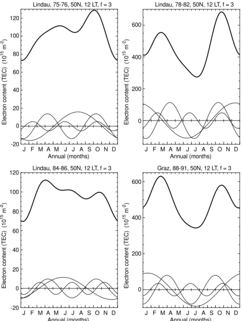
Fig. 3.Annual variation of ionospheric
electron content (TEC) from four Fourier components (mean, 1-year, 1/2-year, 4-months). Low solar activity (R20)
left-hand side, high solar activity (R150)
Table 4.Occurence of the maxima of the annual and semi-annual Fourier components of TEC for solar cycles 21 and 22 Cycle 21. 1978±1982 (HSA:R150), geogr. latitude 50°N
LT interval maximum of the maximum of the
annual component semi-annual component
23±1 ®rst half of June ®rst half of April
1±3 ®rst half of June second half of April
3±5 ®rst half of June second half of April
5±7 second half of June second half of April
7±9 ®rst half of July second half of April
9±11 ®rst half of January second half of April
11±13 ®rst half of December ®rst half of April
13±15 second half of December ®rst half of April
15±17 second half of February ®rst half of April
17±19 ®rst half of May ®rst half of April
19±21 ®rst half of June ®rst half of April
21±23 ®rst half of June ®rst half of April
Cycle 22. 1988±1991 (HSA:R=150), geogr. latitude 50°N
LT interval maximum of the Maximum of the
annual component semi-annual component
23±1 ®rst half of June second half of April
1±3 ®rst half of June ®rst half of June
3±5 ®rst half of June second half of June
5±7 second half of June ®rst half of April
7±9 ®rst half of June ®rst half of April
9±11 second half of February second half of March
11±13 second half of January second half of March
13±15 second half of January ®rst half of April
15±17 second half of March second half of March
17±19 second half of May second half of March
19±21 ®rst half of June second half of March
21±23 ®rst half of June second half of March
Cycle 21. 1975±1976 (LSA:R20), geogr. latitude 50°N
LT interval maximum of the Maximum of the
annual component semi-annual component
23±1 second half of June second half of June
1±3 ®rst half of June second half of June
3±5 second half of June second half of June
5±7 second half of June ®rst half of July
7±9 second half of June ®rst half of March
9±11 second half of July second half of April
11±13 ®rst half of August ®rst half of April
13±15 ®rst half of July ®rst half of April
15±17 second half of June ®rst half of April
17±19 second half of June second half of April
19±21 second half of June ®rst half of June
21±23 ®rst half of July second half of June
Cycle 22. 1984±1986 (LSA:R20), geogr. latitude 50°N
LT interval maximum of the maximum of the
annual component semi-annual component
23±1 second half of June second half of June
1±3 ®rst half of June second half of June
3±5 second half of June second half of June
5±7 second half of June second half of May
7±9 second half of June ®rst half of April
9±11 ®rst half of June second half of April
11±13 ®rst half of June ®rst half of April
13±15 ®rst half of June ®rst half of April
15±17 second half of June second half of March
17±19 second half of June ®rst half of February
19±21 second half of June second half of June
1700 to 1900 LT is a transition between night- and daytime behaviour too (Table 4, Fig. 2, bottom). The change of phase of the annual component is smoother than in cycle 21 and the change occurs earlier for 60N than for 50N.
2.2.2 Semi-annual component
For cycle 21 for LSA the maximum of the semi-annual part shows a dierent position for day and night. At night it occurs around the solstices (1900 to 0700 LT, second half of June), and during the day around the equinoxes (April, October). During the interval 0500± 0700 LT there is a night-to-day change (Table 4).
During the time of HSA the phase of the semi-annual component is very stable (April, October) (Table 4). Only for high latitudes for 0100±0500 LT does the phase change to May (55N) and June (60N). The develop-ment of the ``visibility'' of the autumn maximum occurs later (10 a.m.) than in the following cycle, and disap-pears earlier (Figs. 2 and 4, top).
For cycle 22 for LSA the maximum of the semi-annual part shows almost the same behaviour as during the previous cycle (Table 4). The change from day to night behaviour is more distinct (1700±1900 LT, Feb-ruary).
During the time of HSA the phase of the semi-annual component is very stable too, but in daytime it occurs during this cycle half a month earlier (second half of March, ®rst half of April) (Table 4 and Figs. 2 and 5, bottom). Only for latitudes from 50 to 60N does the
phase change from 0100 to 0500 LT to June (Table 4).
2.2.3 4-month component.
During HSA the 4-month component also visibly in¯uences the annual variation. Cycle 21: the maxima occur at the end of October, February and June and intensify the autumn maximum with the annual varia-tion. Cycle 22: the maxima occur at the begin of March, July and November and strengthen the spring maximum of the annual variation.
3 Long-term behaviour of geomagnetic activity
The long-term behaviour of geomagnetic activity fol-lows roughly the solar activity. However, marked dierences were already found at the beginning of this century (e.g. Cortie, 1912). The maximum of geomag-netic activity is delayed when compared with the maximum of solar activity. Geomagnetic activity has a pronounced annual variation (dominant semi-annual component) whereas solar activity has none (Fraser-Smith, 1972). Re®ned studies revealed that the annual variation of geomagnetic activity is not due to an in¯uence of the atmosphere-ionosphere-magnetosphere system of the earth but is an eect of the earth-sun geometry (compare, e.g. Russell and McPherron, 1973, Triskova, 1989). For the development of the
semi-annual variation there exist two theories: the axial hypothesis (Priester and Cattani, 1962) and the eq-uinoctial hypothesis (Bartels, 1963), which has been used for ionospheric investigations (e.g. Apostolov and Alberca, 1995).
3.1 Vernal-autumnal asymmetry in the seasonal variation of geomagnetic activity
A double-sunspot-cycle variation also occurs in terres-trial magnetic activity (Chernosky, 1966). Chernosky found that in even-numbered cycles the last half of the sunspot-number cycle is more active than the ®rst half, and the converse is true for the odd-numbered cycles. The curve of the 22-year cycle of magnetic activity is not symmetric to the minimum between two cycles. MuÈnch (1972) found an annual wave in the odd-numbered sunspot cycles and explained its generation by an asymmetry in sunspot activity in the two solar hemi-spheres and by the inclination of the sun's equator with respect to the ecliptic. Meyer (1972) investigated C8 character ®gures and found two annual waves to exist in antiphase, with maxima around the equinoxes.
In 1988 the vernal-autumnal asymmetry in the seasonal variation of geomagnetic activity was investi-gated by L. TriskovaÂ. In investigating the variation of geomagnetic activity, not from the viewpoint of solar cycles but with respect to the polarity of the main solar dipole, an annual wave can be observed with maxima alternatively in the periods of vernal and autumnal equinoxes. The phenomenon could be explained by the asymmetry in the main solar dipole ®eld and the result is a stronger in¯uence of the dominant polarity in one of the solar hemispheres. It enhances or attenuates one of the maxima of geomagnetic activity. After 1913 the dominant polarity of the southern solar hemisphere had a greater in¯uence which, under negative polarity (e.g. 1972±1980) enhances, and under positive polarity (e.g. 1960±1969, 1982±1987) attenuates the vernal geomag-netic activity maximum in comparison with the autum-nal one (Triskova, 1989).
3.2 The in¯uence of magnetic activity on mid-latitude F-layer ionization
Graz, 78-82, 50N, 00 LT, f = 6 250 El ect ron cont ent (T EC ) (10 m ) 15 -2 200 150 100 50 0 -50 -100
J F M
Annual (months)
A M J J A S O N D
Graz, 78-82, 50N, 02 LT, f = 6
El ect ron cont ent (T EC ) (10 m ) 15 -2 200 150 100 50 0 -50
J F M
Annual (months)
A M J J A S O N D
Graz, 78-82, 50N, 04 LT, f = 6
El ect ron cont ent (T EC ) (10 m ) 15 -2 150 100 50 0 -50
J F M
Annual (months)
A M J J A S O N D
Graz, 78-82, 50N, 06 LT, f = 6 300 El ect ron cont ent (T EC ) (10 m ) 15 -2 200 100 0 -100
J F M
Annual (months)
A M J J A S O N D
Graz, 78-82, 50N, 08 LT, f = 6
El ect ron cont ent (T EC ) (10 m ) 15 -2 400 300 200 100 0 -100
J F M
Annual (months)
A M J J A S O N D
Graz, 78-82, 50N, 10 LT, f = 6
El ect ron cont ent (T EC ) (10 m ) 15 -2 600 500 400 0 -100
J F M
Annual (months)
A M J J A S O N D 300
200
100
Graz, 78-82, 50N, 12 LT, f = 6
600 El ect ron cont ent (T EC ) (10 m ) 15 -2 400 200 0
J F M
Annual (months)
A M J J A S O N D
Graz, 78-82, 50N, 14 LT, f = 6
El ect ron cont ent (T EC ) (10 m ) 15 -2 600 400 200 0
J F M
Annual (months)
A M J J A S O N D
Graz, 78-82, 50N, 16 LT, f = 6
El ect ron cont ent (T EC ) (10 m ) 15 -2 500 400 0 -100
J F M
Annual (months)
A M J J A S O N D 300
200
100
Graz, 78-82, 50N, 18 LT, f = 6
400 El ect ron cont ent (T EC ) (10 m ) 15 -2 200 100 0 -100
J F M
Annual (months)
A M J J A S O N D
Graz, 78-82, 50N, 20 LT, f = 6
El ect ron cont ent (T EC ) (10 m ) 15 -2 300 200 100 0 -100
J F M
Annual (months)
A M J J A S O N D
Graz, 78-82, 50N, 22 LT, f = 6
El ect ron cont ent (T EC ) (10 m ) 15 -2 0 -100
J F M
Annual (months)
A M J J A S O N D 300
200
100 300
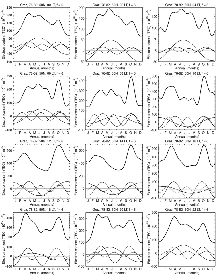
Fig. 4.Annual variation of ionospheric electron content (TEC) for
50N from all 6 Fourier components (mean, 1 year, , 2 months) (Fourier interpolation). The original monthly medians are the TEC values in the middle of each monthly interval. High solar activity
Graz, 88-92, 50N, 00 LT, f = 6 250 El ect ron cont ent (TEC ) (10 m ) 15 -2 200 150 100 50 0 -50 -100
J F M
Annual (months)
A M J J A S O N D
Graz, 88-92, 50N, 02 LT, f = 6
El ect ron cont ent (TEC ) (10 m ) 15 -2 250 150 100 50 0 -100
J F M
Annual (months)
A M J J A S O N D
Graz, 88-92, 50N, 04 LT, f = 6
El ect ron cont ent (TEC ) (10 m ) 15 -2 150 100 50 0 -100
J F M
Annual (months)
A M J J A S O N D
Graz, 88-92, 50N, 06 LT, f = 6 300 El ect ron cont ent (TEC ) (10 m ) 15 -2 200 100 0 -100
J F M
Annual (months)
A M J J A S O N D
Graz, 88-92, 50N, 08 LT, f = 6
El ect ron cont ent (TEC ) (10 m ) 15 -2 300 200 100 0 -100
J F M
Annual (months)
A M J J A S O N D
Graz, 88-92, 50N, 10 LT, f = 6
El ect ron cont ent (TEC ) (10 m ) 15 -2 500 400 300 0 -100
J F M
Annual (months)
A M J J A S O N D
Graz, 88-92, 50N, 12 LT, f = 6
El ect ron cont ent (TEC ) (10 m ) 15 -2 600 400 200 0
J F M
Annual (months)
A M J J A S O N D
Graz, 88-92, 50N, 14 LT, f = 6
El ect ron cont ent (TEC ) (10 m ) 15 -2 600 400 200 0
J F M
Annual (months)
A M J J A S O N D
Graz, 88-92, 50N, 16 LT, f = 6
El ect ron cont ent (TEC ) (10 m ) 15 -2 300 200 100 0 -100
J F M
Annual (months)
A M J J A S O N D
Graz, 88-92, 50N, 18 LT, f = 6 500 El ect ron cont ent (TEC ) (10 m ) 15 -2 400 300 200 100 0 -100
J F M
Annual (months)
A M J J A S O N D
Graz, 88-92, 50N, 20 LT, f = 6
El ect ron cont ent (TEC ) (10 m ) 15 -2 400 300 200 100 0 -100
J F M
Annual (months)
A M J J A S O N D
Graz, 88-92, 50N, 22 LT, f = 6
El ect ron cont ent (TEC ) (10 m ) 15 -2 300 200 100 0 -100
J F M
Annual (months)
A M J J A S O N D 200 -50 200 250 -50 100 200 400 500
number density ratio [0]/[N2], which also leads to a depression of ionization because recombination is enhanced as compared with production. The ``negative storm eect'' is a typical phenomenon which is observed on the day following the day of the onset of a geomagnetic storm. In general it is observed in connec-tion with moderate and severe geomagnetic storms. Usually the mid-latitude F-layer reaction to weak storms and to substorms is not directly observable because weak eects are masked by ionization variations not related to geomagnetic activity (day-to-day variabil-ity, TIDs, etc.). Experience with a large amount of European data (electron content, peak density) shows that ``positive storm eects'', which can occur in the afternoon when the onset of the geomagnetic storm is in the (early) morning, do not cancel out the ``negative eects''. We have reason to believe that the statistical eect of geomagnetic disturbances on F-layer ionization in (European) mid-latitudes is a depression of ioniza-tion. Therefore the annual asymmetry of F-layer ionization in mid-latitudes should be in anti-phase with the vernal-autumnal asymmetry of geomagnetic activity. This is what we have observed.
The dominance of negative storm eects in summer was shown by Putz et al. (1990) for three European stations. At Stanford, USA (35N), in summer, the negative eects were much larger than the positive ones (Titheridge and Buonsanto, 1988). Only in winter can positive eects dominate (Putz et al., 1990; Titheridge and Buonsanto, 1988). Since no reports on statistical studies of equinoctial storms were found, we made an investigation of the eect of geomagnetic disturbances in the following way. Long series of the quantity
D NmaxÿNmax=Nmax were calculated for given local time and compared with the daily geomagnetic distur-bance indexAp (Nmax: monthly average). To account for the delay of ionospheric eects compared with geomag-netic eects we took theApof the previous day. For each month we calculated the sum ofDwhen Ap was greater than a limit value. For theNmaxdata from Rome, Italy, from the time-interval 1958 through to 1994 we obtained, with Ap limits between 5 and 30, very stable results: only winter sums ofDare positive, all the others negative. No dierence was found between the months around the equinoxes (March, April, September, Octo-ber) and summer. The D sum for the whole year is strongly negative.
We do not want to rule out other possibilities to explain the double sunspot cycle observed in electron content and in peak density, but it is unlikely that a pure solar-activity explanation can be found. There is no reason to believe in seasonal changes of the relation of a solar-activity indicator to the solar EUV output.
4 Discussion of the results
Our investigation of two consecutive cycles (cycle 21 and 22) indicates the existence of a 22-year period in the daytime TEC of the ionosphere. During cycle 21 the maximum of the annual variation shows a distinct
autumn maximum. During cycle 22 this occurs in spring. This change is caused by a shift of the annual component with respect to the semi-annual component of one or two months during daytime. (Only during this time-interval the semi-annual component is evident: Figs. 4 and 5.) We got the same results for LSA and HSA.
For LSA of cycle 21 the maximum of the annual component occurs later in summer and therefore sup-ports the development of an autumn maximum. For HSA of cycle 21 the maximum slips to the ®rst half of winter (December, January) and causes the same eect. The autumn maximum (cycle 21) and the spring maximum (cycle 22) is additionally increased by the same-season maximum of the 4-month component. The change of the time of the maximum is supported by data and descriptions published in previous publications for cycles 20 and 21 (Yuen and Roelof, 1967; da Rosaet al., 1973; Huang, 1979). The paper by Garriottet al. (1970) displays electron content from the Faraday eect on the signals of ATS-1. The data from 1968 show a clear spring maximum both for Stanford (34:2N, 234.5E) and Hawaii (19:8N, 202:8E). 1968 was a year with
fairly uniform solar activity (103R12111). Our
Fourier analysis for the Stanford 1968 data is shown in Fig. 6. (Compare also Titheridge et al., 1996.)
For Europe, GaldoÂn and Alberca (1970) show a spring maximum for 1965, 1966 and 1967 (Tortosa, 40:8N, 0:5E; cycle 20). The vernal-equinox values
exceed the autumnal ones by more than a factor of 2. We suspect an overestimation because of arti®cial enhancement by the normalization to a constant level of solar activity. The European data were gained by means of the Faraday eect on the 40/41-MHz signals of
Stanford, 1968, 34N, 14 LT, f = 3 500
El
ect
ron
cont
ent
(T
EC
)
(10
m
)
15
-2
400
300
200
100
0
-100
J F M A M J
Annual (months)
J A S O N D
Fig. 6.Annual variation of ionospheric electron content (TEC) from
a low orbiting satellite (Explorer 22) which coupled diurnal and annual variation.
A comparison with the southern hemisphere brought no results for our investigations (Titheridgeet al., 1996). There seems to be no marked dierence between vernal and autumnal maximum in the southern hemisphere.
The investigation of the annual variation of peak electron density (Nmax: Fig. 7) also indicates the exis-tence of a 22-year cycle in daytime F-layer ionization (considering data as early as solar cycle 19).
We show results for Rome (41:8N, 12:5E ± Fig. 7) and remark that the amplitude of the 22-year period-icity gets weaker when the latitude of the ionosonde station is increased [e.g. when the results for Slough (51:5N, ÿ0:6E) are compared with those for Rome].
This seems to correspond with a decrease in the ratio of the amplitudes of the semi-annual component
com-pared with the annual component (for TEC compare Fig. 2).
No distinct and persistent double-sunspot-cycle be-haviour can be found for solar activity. In particular there is no signi®cant semi-annual component in solar-activity spectra. There is no indication of an annual variation in the relation between a solar-activity indica-tor (based on sunspot numbers or on solar radio ¯ux) and the EUV output of the sun.
But, as already mentioned, the double-sunspot-cycle variation also occurs in terrestrial magnetic activity. Edwin Chernosky found an even cycle-odd cycle asym-metry in the average of ``disturbed-day occurrence'' from grouped data for 1884±1963 (Chernosky, 1966). Ludmila Triskova detected a very clear vernal-autumnal asym-metry in the average annual variation of theaaindex (see Mayaud, 1972) and a change of the maximum from spring in odd cycles to autumn in even cycles. This
58-64 d, 14 LT, R12 = 150, f = 3
P
eak
el
ect
ron
densi
ty
(Nm
ax)
(10
m
)
10
-3 150
100
50
0
J F M A M J
Annual (months) Nmax Rome
J A S O N D
69-74 d, 14 LT, R12 = 150, f = 3
P
eak
el
ect
ron
densi
ty
(Nm
ax)
(10
m
)
10
-3
150
100
50
0
J F M A M J
Annual (months) Nmax Rome
J A S O N D
76-80 u, 14 LT, R12 = 150, f = 3
P
eak
el
ect
ron
densi
ty
(Nm
ax)
(10
m
)
10
-3
150
100
50
0
J F M A M J
Annual (months) Nmax Rome
J A S O N D
80-85 d, 14 LT, R12 = 150, f = 3
P
eak
el
ect
ron
densi
ty
(Nm
ax)
(10
m
)
10
-3
150
100
50
0
J F M A M J
Annual (months) Nmax Rome
J A S O N D 250
200
-50
200 250
200
-50
Fig. 7.Annual variation of peak electron
behaviour was demonstrated for these parts of the solar cycles from 1873 to 1980 which have a well-developed solar dipole polarity (Triskova, 1989).
An analysis of monthly medians of aa from solar cycles 18±23 using essentially the Fourier method was applied to the TEC, andNmaxdata shows that the phase of the annual component might be responsible for the 22-year period in geomagnetic activity (Fig. 8).
This aa-index behaviour might provide a basis for explanations of the double sunspot cycle in the total electron of the ionosphere, because the geomagnetic activity certainly in¯uences the ionospheric behaviour.
Qualitatively the relation between magnetic activity (described by a magnetic-activity indicator) and F-layer ionization can be explained by means of varying energy input into the high-latitude thermosphere (Joule heating and other particle precipitation eects). Quantitative explanations are a dicult task; for instance, the magnetic activity indicators available for long-term investigations have no direct relation to particle precip-itation nor to current systems.
References
Apostolov, E. M., and L. F. Alberca,foF2 hysteresis variations and
the semi-annual geomagnetic wave.J. Atmos. Terr. Phys, 57, 755±757, 1995.
Baranyi, T., and A. LudmaÂny, Semi-annual ¯uctuation and
eciency factors in sun-weather relations, J. Geophys. Res., 97,14923±14928, 1992.
Baranyi, T., and A. LudmaÂny, Role of the solar main magnetic
dipole ®eld in the solar-tropospheric relations. Part I. Semian-nual ¯uctuations in Europe, Ann. Geophysicae, 13, 427±436, 1995a.
Baranyi, T., and A. LudmaÂny, Role of the solar main magnetic
dipole ®eld in the solar-tropospheric relations. Part II. Depen-dence on the types of solar sources,Ann. Geophysicae,13,886± 892, 1995b.
Bartels, J.,Discussion of time-variations of geomagnetic activity,
indices Kp and Ap, 1932±1961,Ann. GeÂophys.,19,1±20, 1963.
Chernosky, E. J., Double sunspot-cycle variation in terrestrial
magnetic activity 1884±1963, J. Geophys. Res., 71, 965±974, 1966.
Cortie, A. L.,Sunspots and terrestrial magnetic phenomena, 1898±
1911,Mon. Not. R. Astron. Soc.,73,52±60, 1912.
da Rosa, A. V., H. Waldman, and J. Bendito, Response of the
ionospheric electron content to ¯uctuations in solar activity,J. Atmos. Terr. Phys.,35,1429±1442, 1973.
Ebel, A.,Temporal and spatial changes of the electron content of
the ionosphere,J. Atmos. Terr. Phys.,32,1649±1660, 1970.
Ebel, A., Der ionosphaÈrische Elektroneninhalt und seine
weltwei-ten langperiodischen AÈnderungen,Mitt. Inst. Geophys. Mete-orol. Univ. KoÈln,17,1971.
Feichter, E., and R. Leitinger, Long-term studies of ionospheric
electron content, Wiss. Ber. 1/93, Institut fuÈr Meteorologie und Geophysik, UniversitaÈt Graz, 1993.
Feichter, E., R. Leitinger, and G. K. Hartmann,Untersuchungen
uÈber die Halbjahres- und die Jahreswelle in F-Schicht-Parame-tern,Kleinheubacher Ber.,31,249±258, 1988.
Feichter, E., R. Leitinger, and G. K. Hartmann, Vergleich von
IonosphaÈrenparametern aus zwei Sonnen¯eckenzyklen, Klein-heubacher Ber,33,93±102, 1990.
Feichter, E., R. Leitinger, and G. K. Hartmann,Die
Halbjahres-periode in der ThermosphaÈre und in der IonosphaÈre ± ein Vergleich,Kleinheubacher Ber,34,207±214, 1991.
Fraser-Smith, A. C.,Spectrum of the geomagnetic activity index
Ap,J. Geophys. Res.,77,4209±4220, 1972.
Garriot, O. K., A. V. da Rosa, and W. J. Ross.Electron content
obtained from Faraday rotation and phase path length variations. J. atmos. terr. Phys.32,705±727, 1970
GaldoÂn, E., and L. F. Alberca,In¯uence of solar activity on the
total electron content of the ionosphere over Tortosa,Radio Sci.,3,913±915, 1970.
Huang,Y. -N.,Solar cycle and seasonal variations of the solar and
lunar daily variations of total electron content at Lunping,J. Geophys. Res.,84,6595±6601, 1979.
Leitinger, R., and E. Putz,Die Auswertung von
Dierenz-Doppler-Messungen an den Signalen von Navigationssatelliten, Techn Bericht, UniversitaÈt Graz, 1978.
Leitinger, R., G. Schmidt, and A. Tauriainen,An evaluation method
combining the dierential Doppler measurements from two stations that enables the calculation of the electron content of the ionosphere,J. Geophys,41,201±213, 1975.
Mayaud, P. N.,Theaaindices: a 100-year series characterizing the
magnetic activity,J. Geophys. Res.,77,6870, 1972.
Average aa index for even cycles, f = 6 10
5
0
-5
J F M A M J
Annual (months)
J A S O N D -10
Average aa index for odd cycles, f = 6 10
5
0
-5
J F M A M J
Annual (months)
J A S O N D -10
Fig. 8.Annual deviation from mean of theaa
Meyer, J.,A 12±month wave in geomagnetic activity,J. Geophys. Res.,77,3566±3572, 1972.
MuÈnch, J. W.,The annual variation of the earth-magnetic activity
according to the character ®gures Ci, Planet. Space Sci., 20, 225±231, 1972.
Priester, W., and D. Cattani, On the semiannual variation of
geomagnetic activity and its relation to the solar corpuscular radiation,J. Atmos. Sci.,19,121±126, 1962.
ProÈlss, G. W., Storm-induced changes in the thermospheric
composition at middle latitudes, J. Planet. Space Sci., 35, 807±811, 1987.
ProÈlss, G. W., and M. Roemer,Thermospheric storms,Adv. Space
Res.,7,(10)223±(10)235, 1987.
Putz, E., N. Jakowski, and P. Spalla,Statistische Untersuchungen
von IonosphaÈrenstuÈrmen und erste Modellrechnungen, Klein-heubacher Ber.,33,121±129, 1990.
Russell, C. T., and R. L. Mc Pherron, Semi-annual variation of
geomagnetic activity,J. Geophys. Res.,78,92±108, 1973.
Taeusch, D. R., G. R. Carignan, and C. A. Reber, Neutral
composition variations above 400 km during a magnetic storm,
J. Geophys. Res.,76,8318±8325, 1971.
Titheridge, J. E. and M. J. Buonsanto,A comparison of northern
and southern hemisphere TEC storm behaviour,J. Atmos. Terr. Phys.,50,763±780, 1988.
Titheridge, J. E., R. Leitinger, and E. Feichter,Comparison of the
long-term behaviour of the F-layer of the ionosphere, northern versus southern hemisphere, Kleinheubacher Ber.,39,749±755, 1996.
Triskova, L., The vernal-autumnal asymmetry in the seasonal
variation of the magnetic activity, J. Atmos. Terr. Phys., 51, 111±118, 1989.
Yuen, P. C., and T. H. Roelofs,Seasonal variations in ionospheric
![Table 2. Monthly mean sunspot numbers R for the cycle-22 solar maximum period 1988±1992 [<: R < 120 (not selected), >: R > 180 (not selected)]](https://thumb-eu.123doks.com/thumbv2/123dok_br/18174630.330346/2.918.68.435.135.276/table-monthly-sunspot-numbers-maximum-period-selected-selected.webp)