A Compact Finite Difference Method for Solving the General Rosenau-RLW Equation

A Compact Finite Difference Method for Solving

the General Rosenau–RLW Equation

Ben Wongsaijai, Kanyuta Poochinapan

∗

, and Thongchai Disyadej

Abstract—In this paper, a compact finite difference method to solve the Rosenau–RLW equation is proposed. A numerical tool is applied to the model by using a three–level average implicit finite difference technique. The fundamental conser-vative property of the equation is preserved by the presented numerical scheme, and the existence and uniqueness of the numerical solution are proved. Moreover, the convergence and stability of the numerical solution are also shown. The new method gives second– and fourth–order accuracy in time and space, respectively. The algorithm uses five–point stencil to approximate the derivatives for the space discretization. The numerical experiments show that the proposed method improves the accuracy of the solution significantly.

Index Terms—finite difference method, Rosenau–RLW equa-tion.

I. INTRODUCTION

A

nonlinear wave phenomenon is the important area of scientific research, which many scientists in the past have studied about mathematical models explaining the wave behavior. There are mathematical models which describe the dynamic of wave behaviors–for example, the KdV equation, the RLW equation, the Rosenau equation, and many others [1]–[10]. The KdV equation has been used in very wide applications, such as magnetic fluid waves, ion sound waves, and longitudinal astigmatic waves [4]–[6]. The RLW equation, which was first proposed by Peregrine [7], [8] provides an explanation on a different situation of a nonlinear dispersive wave from the more classical KdV equation. The RLW equation is one of models which are encountered in many areas, e.g. ion–acoustic plasma waves, magnetohydro-dynamic plasma waves, and shallow water waves. Since the case of wave–wave and wave–wall interactions cannot be described by the KdV equation, Rosenau [9], [10] proposed an equation for describing the dynamic of dense discrete systems; it is known as the Rosenue equation. The existence and uniqueness of the solution for the Rosenau equation were proved by Park [11], [12]. For the further consideration of the nonlinear wave, a viscous termuxxtneeds to be included:

ut−uxxt+uxxxxt+ux+ (up)x= 0, (1)

where p ≥ 2 is an integer and u0(x) is a known smooth function. This equation is usually called the Rosenua–RLW equation. Ifp= 2, then Eq. (1) is called the usual Rosenau– RLW equation. Moreover, if p = 3, then Eq. (1) is called the modified Rosenau–RLW equation. The behavior of the

∗

Kanyuta Poochinapan, Corresponding Author, Department of Mathemat-ics, Faculty of Science, Chiang Mai University, Chiang Mai 50200, Thailand (email: kanyuta@hotmail.com, k.poochinapan@gmail.com)

Ben Wongsaijai, Department of Mathematics, Faculty of Science, Chiang Mai University, Chiang Mai 50200, Thailand (email: ben.wongsaijai@gmail.com)

Thongchai Disyadej, Electricity Generating Authority of Thailand, Phit-sanulok 65000, Thailand (e-mail: thongchai.d@egat.co.th)

solution to the Rosenau–RLW equation with the Cauchy problem has been well studied for the past years [13]–[18]. It is known that the solitary wave solution for Eq. (1) is

u(x, t) =eln{(p+3)(3p+1)(p+1)/[2(p2+3)(p2+4p+7)]}/(p+1)×

sech4/(p+1)

"

p−1 p

4p2_{+ 8p+ 20}(x−ct) #

,

wherep≥2is an integer andc= (p4+ 4p3+ 14p2+ 20p+ 25)/(p4_{+ 4p}3_{+ 10p}2_{+ 12p+ 21).}

The Rosenau–RLW equation has been solved numerically by various methods (for example, see [13]–[18]). Zuo et al. [13] have proposed the Crank–Nocolson finite difference scheme for the equation. The convergence and stability of the proposed method were also discussed. Obviously, the scheme in [13] requires heavy iterative computations because the scheme is nonlinear implicit. Pan and Zhang [14], [15] developed linearized difference schemes which are three– level and conservative implicit for both the usual Rosenau– RLW (p = 2) and the general Rosenau–RLW (p ≥ 2)

equations. The second–order accuracy and unconditional stability were also proved.

In this paper, we consider the following initial–boundary value problem of the general Rosenau–RLW equation with an initial condition:

u(x,0) =u0(x), (xl≤x≤xr), (2)

and boundary conditions

u(xl, t) =u(xr, t) = 0,

uxx(xl, t) =uxx(xr, t) = 0, (0≤t≤T). (3)

The initial–boundary value problem possesses the following conservative properties:

Q(t) = Z xr

xl

u(x, t)dx= Z xr

xl

u0(x,0)dx=Q(0),

and

E(t) =kuk2L2+kuxk

2

L2+kuxxk

2

L2 =E(0).

When −xl ≫ 0 and xr ≫ 0, the initial–boundary value

problem (1)–(3) is consistent, so the boundary condition (3) is reasonable.

method is applied in the present research since conservative approximation analysis by the mathematical tools has been developing until now.

The content of this paper is organized as follows. In the next section, we describe a conservative implicit finite difference scheme for the general Rosenau–RLW equation (1) with the initial and boundary conditions (2)–(3). Some preliminary lemmas and discrete norms are given and the invariant property Qn is proved. We discuss about the solvability of the finite difference scheme, and the existence and uniqueness of the solution are also proved in the Section 3. Section 4 presents complete proofs on the convergence and stability of the proposed method with convergence rate O(τ2_+h4_{). The results of validation for the finite difference}

scheme are presented in Section 5, where we make a detailed comparison with available data, to confirm and illustrate our theoretical analysis. Finally, we finish our paper by concluding remarks in Section 6.

II. FINITEDIFFERENCESCHEME

In this section, we introduce a finite difference scheme for the formulation of Eqs. (1)–(3). The solution domain

Ω = {(x, t)| xl ≤ x ≤ xr, 0 ≤ t ≤T} is covered by a

uniform grid:

Ωh={(xi, tn)|xi=xl+ih, tn =nτ,0≤i≤M,

0≤n≤N},

with spacings h = (xr−xl)/M and τ = T /N. Denote

un

i ≈u(xi, tn),

¯

Ωh={(xi, tn)|xi=xl+ih, tn=nτ, −1≤i≤M+ 1,

0≤n≤N},

andZ0

h={un= (uni)|u0=uM = 0, −1≤i≤M + 1}.

We use the following notations for simplicity:

un+12

i =

un_i+1+un i

2 , u¯

n

i =

un_i+1+un_i−1

2 ,

(uni)t=

un_i+1−un i

τ , (u

n i)ˆt=

un_i+1−un_i−1

2τ ,

(uni)x=

un i+1−uni

h , (u

n i)¯x=

un i −uni−1

h ,

(uni)ˆx=

un

i+1−uni−1 2h , (u

n_{, v}n_{) =h} M−1

X

i=1

univni,

kunk2= (un, un), kunk∞= max

1≤i≤M−1|u

n i|.

By setting w=uxxt−ux−uxxxxt−(up)x, Eq. (1) can be

written asw=ut. By the Taylor expansion, we obtain

wn

i = (∂tu)ni = (uni)ˆt+O

¡

τ2¢

, (4)

and

wni =

·

(uni)xx¯ˆt−

h2 12 ¡

∂x4∂tu¢ n i

¸

−

·

(uni)xˆ−

h2 6

¡

∂x3u

¢n

i

¸

−

·

(uni)xxx¯x¯ˆt−

h2 6

¡

∂6x∂tu¢ n i

¸

−

· [(uni)

p

]_xˆ−h

2

6 ¡

∂x3up

¢n

i

¸ +O¡

h4¢

. (5)

From Eq. (4), we have

¡

∂6

x∂tu¢ n

i =

¡

∂4

x∂tu¢ n i − ¡ ∂3 xu ¢n i− ¡ ∂3

xup

¢n i− ¡ ∂2 xw ¢n

i . (6)

Then,

wn

i =

· (un

i)xx¯ˆt−

h2 12 ¡

∂4

x∂tu¢ n i

¸

−

· (un

i)xˆ−

h2 6 ¡ ∂3 xu ¢n i ¸ − · [(un

i) p

]_xˆ−h

2

6 ¡

∂3

xup

¢n

i

¸

−

· (un

i)xxx¯x¯ˆt

−h

2

6 h

¡

∂x4∂tu¢ n

i −

¡

∂x3u

¢n

i −

¡

∂3xup

¢n

i −

¡

∂2xw

¢n

i

i¸

+O¡

h4¢

. (7)

This implies that

win= (uni)xx¯ˆt+

h2 12 ¡

∂x4∂tu¢ n i −(u

n

i)xˆ−[(uni) p

]ˆx

−(uni)xxx¯¯xtˆ−

h2 6

¡

∂x2w

¢n

i +O

¡

h4¢

. (8)

Using second–order accuracy for approximation, we obtain

¡

∂4xu

¢n

i =(u n

i)xxx¯x¯+O ¡

h2¢

,

¡

∂x2w

¢n

i = (w n i)x¯x+O

¡

h2¢

.

The following method is a proposed finite difference scheme to solve the problem (1)–(3):

(uni)ˆt−

µ 1−h

2

6 ¶

(uni)x¯xˆt+

µ 1−h

2

12 ¶

(uni)xxx¯x¯ˆt

+ (un

i)ˆx+ [(uni) p

]_xˆ= 0;

1≤i≤M −1, 1≤n≤N−1, (9)

where

u0

i =u0(xi), 0≤i≤M, (10)

un0 =unM = 0, (un0)xx¯= (unM)x¯x= 0, 1≤n≤N.

(11)

A three–step method is used for the time discretization of the above described scheme. After the new time discretiza-tion of Eq. (9) is performed, three– and five–point stencils approximating the derivatives for the space discretization are used to obtain an algebraic system. The matrix system of Eq. (9) is banded with penta–diagonals and we use a standard routine of the MATLAB to solve the system (9)–(11). The nonlinear term of Eq. (1) is handled by using the linear implicit scheme. Therefore, the equations are solved easily by using the presented method since it does not require extra effort to deal with the nonlinear term.

Lemma 1: (Pan and Zhang [15]) For any two mesh func-tionsu, v∈Z0

h, we have

(uxˆ, v) =−(u, vˆx),

(ux, v) =−(u, v¯x),

(v, uxx¯) =−(vx, ux),

(u, uxx¯) =−(ux, ux) =−kuxk2.

Furthermore, if(un

0)xx¯= (unM)x¯x= 0, then it implies

Theorem 2: Suppose thatu0∈H02, then the scheme (9)–

(11) is conservative in sense:

Qn = h 2

M−1 X

i=1 ¡

uni+1+uni

¢

= Qn−1 =. . . =Q0, (12)

under assumptions u−1=u1= 0anduM−1=uM+1= 0. Proof: By multiplying Eq. (9) byh, summing up for i from0 toM−1, considering the boundary conditions, and assuming u−1=u1= 0anduM−1=uM+1= 0, we get

h

2

M−1 X

i=1 ¡

uni+1−uni−1

¢ = 0.

Then, this gives Eq. (12).

Lemma 3: (Discrete Sobolev’s inequality [21]) There exist two constants C1 andC2 such that

kunk∞≤C1kunk+C2kunxk.

Theorem 4: Suppose u0 ∈ H02[xl, xr], then the solution

un _{satisfies ku}n_{k ≤ C and ku}n

xxk ≤ C, which yields kun_k

∞≤C .

Proof: It follows from the initial condition (10) that u0_{≤C. The first levelu}1 _{is computed by the fourth–order}

method. Hence, the following estimates are gotten about

° °u1

°

° ≤ C and ° °u1

°

°_∞ ≤ C. Now, we use the induction

argument to prove the estimate. We assume that

° °uk

° °

∞≤C for k= 0,1,2, . . . , n. (13)

Taking the inner product of Eq. (9) with 2¯un _{and using}

Lemma 1, we obtain

° °un+1

° ° 2

−° °un−1

° ° 2

+ µ

1−h

2

6 ¶

³_° °un_x+1

° ° 2

−° °un_x−1

° °

2´

+ µ

1−h

2

12 ¶

³_° °un_xx+1_¯

° ° 2

−° °un_xx−_¯1

° °

2´

=−2τ((un)_xˆ,2¯un)−2τ([(un)p]_xˆ,2¯un).

According to the Cauchy–Schwarz inequality and direct calculation, it gives

kunxˆk ≤ kunxk,

and

((un)xˆ,2¯un)≤ µ

kunxk

2 +1

2 ° °un+1

° ° 2 +1 2 ° °un−1

° °

2¶

.

From Eq. (13), the Cauchy–Schwarz inequality, and Lemma 1, we get

([(un)p]xˆ,2¯un) =−h

M−1 X

i=1 (uni)

p¡

uni+1+uni−1

¢ ˆ

x

≤C

µ

kunk2+1 2

° °un_x+1

° °2+

1 2 ° °un_x−1

° °2

¶

.

Setting

Bn =kunk2+° °un−1

° ° 2

+ µ

1−h

2

6 ¶

³

kunxk

2 +°

°un_x−1 ° °

2´

+ µ

1−h

2

12 ¶

³

kunxx¯k 2

+° °un_x−_¯x1

° °

2´

,

then

Bn+1−Bn≤τ C¡

Bn+1+Bn¢

.

If τ is sufficiently small, which satisfies τ ≤ k−2

kC and

k >2, then

Bn+1≤ (1 +τ C)

(1−τ C)B

n_{≤(1 +τ kC)B}n_{≤exp (kCT)B}0_.

Hence°°un+1 ° °≤C,

° °un_x+1

°

°≤C, and ° °un_x+1_¯x

°

°≤C, which

yield°°un+1 °

°_∞≤C by Lemma 3.

III. SOLVABILITY

In this section, we prove the existence and uniqueness of our proposed scheme that implies the unique solvability.

Theorem 5: The finite difference scheme (9)–(11) is uniquely solvable.

Proof: By using the mathematical induction, we can determine u0 _{uniquely by an initial condition and then}

choose a fourth–order method to computeu1_{. Now, suppose}

u0_{, u}1_{, u}2_{, ..., u}n _{to be solved uniquely. By considering Eq.}

(9) forun+1_{, we have}

1 2τu

n+1

i −

1 2τ

µ 1−h

2

6 ¶

¡

un_i+1¢

xx¯+

1 2τ

µ 1−h

2

12 ¶

¡

un_i+1¢

xx¯xx¯= 0. (14)

By taking an inner product of Eq. (14) withun+1_{, we obtain}

1 2τ

° °un+1

° ° 2 − 1 2τ µ 1−h

2

6 ¶

° °un_x+1

° ° 2 + 1 2τ µ 1−h

2

12 ¶

° °un_xx+1_¯

° ° 2

= 0.

By the Cauchy–Schwarz inequality and Lemma 1, we have

° °un_x+1

° ° 2

= (un+1, unxx+1¯ )≤ 1 2 ° °un+1

° ° 2 +1 2 ° °un_x+1_¯x

° ° 2 . Then, 1 2 ° °un+1

° ° 2 + µ 1 2− h2 12 ¶ ° °un_xx+1_¯

° ° 2

= 0.

Therefore, Eq. (14) has the only one solution and Eq. (9) un+1 _{is uniquely solvable. This completes the proof of}

Theorem 5.

IV. CONVERGENCE AND STABILITY

In this section, we prove the convergence and stability of the scheme (9)–(11). Let en

i =vni −uin, where vni and uni

are the solutions of (1)–(3) and (9)–(11), respectively. Then, we obtain the following error equations:

rin= (eni)ˆt−

µ 1−h

2

6 ¶

(eni)xx¯ˆt+

µ 1−h

2

12 ¶

(eni)xxx¯x¯ˆt

+ (eni)xˆ+ [(v

n i)

p

]_ˆx−[(uni) p

]_xˆ, (15)

wherern

i denotes the truncation error. By using the Taylor

expansion, it is easy to see that rn

i =O(τ2+h4) holds as

τ, h→0. The following lemmas are essential for the proof of convergence and stability of our scheme.

Lemma 6: (Discrete Gronwall’s inequality [21]) Suppose that ω(k) and ρ(k) are nonnegative functions and ρ(k) is nondecreasing. IfC >0 and

ω(k)≤ρ(k) +Cτ

k−1 X

l=0

then

ω(k)≤ρ(k)eCτ k, ∀k.

Lemma 7: (Pan and Zhang [15]) Suppose that u0 ∈

H2

0[xl, xr], then the solutionun of Eqs. (1)–(3) satisfies kukL2 ≤C, kuxkL2 ≤C,

kuxxkL2≤C, kukL∞ ≤C.

The following theorem shows that our scheme converges to the solution with convergence rateO(τ2_+h4_).

Theorem 8: Suppose u0 ∈ H02[xl, xr], then the solution

un _{converges to the solution for the problem in the sense of} k·k_∞ and the rate of convergence isO(τ2_+h4_).

Proof:By taking an inner product on both sides of Eq. (15) with2¯en≡(en+1+en−1), we get

³_° °en+1

° ° 2

−°°en−1 ° °

2´ +

µ 1−h

2

6 ¶

³_° °en_x+1

° ° 2

−°°en_x−1 ° °

2´

+ µ

1−h

2

12 ¶

³_° °en_x+1_x¯

° ° 2

−°°en_x−_¯x1 ° °

2´

= 2τ(rn,2¯en)

−2τ(enxˆ,2¯en)−2τ([(vn)

p

]_xˆ−[(un)p]_xˆ,2¯en). (16)

According to the Schwarz inequality, Lemma 1, Theorem 2, and Lemma 7, we obtain

µ [(vn₎p

]_xˆ−[(un₎p

]_ˆx,2¯en

¶

= 2h

M−1 X

i=1 ·

[(vn i)

p

]_xˆ−[(un i)

p

]_ˆx ¸

¯

en i

=−2h

M−1 X

i=1 ·

(vn i)

p −(un

i) p¸

(¯en i)xˆ

= 2h

M−1 X

i=1 ·

eni p−2 X

k=1 (vin)

p−k−2 (uni)

k¸

(¯eni)xˆ

≤C³kenk2+ke¯nxˆk 2´

≤C

µ

kenk2+° °en_xˆ−1

° ° 2

+° °en_xˆ+1

° °

2¶

. (17)

By the Cauchy–Schwarz inequality, Lemma 1, and a direct calculation, we obtain

kenxˆk ≤ kenxk, (18)

kenxk=−(en, enx¯x)≤

1 2

³

kenk2+kenx¯xk

2´

, (19)

(enxˆ,2¯en)≤ kenˆxk

2 +1

2 ³_°

°en+1 ° ° 2

+°°en−1 ° °

2´

, (20)

(rn,2¯en)≤ krnk2+1 2

³_° °en+1

° ° 2

+° °en−1

° °

2´

. (21)

From Eqs.(16)–(21), they yield

³_° °en+1

° ° 2

−°°en−1 ° °

2´

+ µ

1−h

2

6 ¶_³

° °en_x+1

° ° 2

−° °en_x−1

° °

2´

+ µ

1−h

2

12 ¶_³

° °en_xx+1_¯

° ° 2

−° °en_x−_x¯1

° °

2´

≤2τkrn_k2_{+τ C} µ

° °en−1

° ° 2

+ken_k2 +°

°en+1 ° ° 2

+° °en_x−1

° ° 2

+kenxk

2 +°

°en_x+1 ° °

2¶

. (22)

Setting

En_=ken_k2 +°

°en−1 ° ° 2

+ µ

1−h

2

6 ¶_³

ken xk

2 +°

°en_x−1 ° °

2´

+ µ

1−h

2

12 ¶_³

ken xx¯k

2 +°

°en_xx−_¯1 ° °

2´

,

then Eq. (22) can be rewritten as

En+1−En≤2τkrnk2+τ C¡

En+1+En¢

,

and

(1−2τ C)¡

En+1−En¢

≤τkrnk2+ 2τ CEn.

Ifτ is sufficiently small, which satisfies1−2Cτ >0, then

En+1−En≤τ Ckrnk2+τ CEn. (23)

Summing up Eq. (23) from1 ton, we have

En+1≤E1+Cτ

n

X

k=1 ° °rk

° ° 2 +Cτ n X k=1

Ek. (24)

Thus, we can use a fourth–order method to computeu1_such

that

E1≤O(τ2+h4)2,

and τ n X k=1 ° °rk

° ° 2

≤nτ max 0≤l≤n−1

° °rl

° ° 2

≤T·O(τ2+h4)2.

By Lemma 6, we obtainEn_≤O(τ2_+h4₎2_{, that is}

kenk ≤O(τ2+h4), kenxx¯k ≤O(τ2+h4).

From Eq. (20), we obtain

ken_{k ≤O(τ}2_+h4_{), ke}n

xk ≤O(τ2+h4),

and

kenx¯xk ≤O(τ2+h4).

By Lemma 3,

kenk_∞≤O(τ2+h4).

This completes the proof.

Theorem 9: Under the conditions of Theorem 8, the so-lutionun _{of Eqs. (9)–(11) is stable in normk · k}

∞.

V. NUMERICALEXPERIMENTS

In this section, we present numerical experiments on a test problem to confirm and illustrate the accuracy of our proposed method. The accuracy of the method is measured by the comparison of numerical solutions with exact solu-tions as well as other numerical solusolu-tions from the method in the literature [15] by using k · k and k · k∞ norm. The initial condition associated for the Rosenau–RLW equation takes the form:

u0(x) =eln{(p+3)(3p+1)(p+1)/[2(p2+3)(p2+4p+7)]}/(p+1)×

sech4/(p+1)

"

p−1 p

4p2_{+ 8p+ 20}(x) #

TABLE I

COMPARISON OF ERRORS WITHτ= 0.1,h= 0.25,xl=−60,AND xr= 120ATt= 40.

kek ×10−2

kek∞×10 −3

p Present Pan&Zhang Present Pan&Zhang

2 0.23608 0.78777 0.88670 2.88972

4 0.47254 1.73066 1.81252 6.47969

8 0.46713 1.80583 1.75739 6.66740

16 0.38438 1.37857 1.30630 5.05919

TABLE II

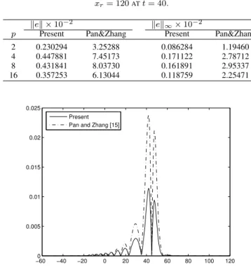
COMPARISON OF ERRORS WITHτ= 0.1,h= 0.5,xl=−60,AND xr= 120ATt= 40.

kek ×10−2

kek∞×10 −2

p Present Pan&Zhang Present Pan&Zhang

2 0.230294 3.25288 0.086284 1.19460

4 0.447881 7.45173 0.171122 2.78712

8 0.431841 8.03730 0.161891 2.95337

16 0.357253 6.13044 0.118759 2.25471

−600 −40 −20 0 20 40 60 80 100 120

0.005 0.01 0.015 0.02 0.025

Present Pan and Zhang [15]

Fig. 1. Absolute error distribution atp= 4, h= 0.5, τ=h2

, andt= 40.

For u1_{, we employ a two–level method to estimate the}

solution by

(uni)t−

µ 1−h

2

6 ¶

(uni)xxt¯ + µ

1−h

2

12 ¶

(uni)xx¯xxt¯

+³un_i+12´

ˆ

x+ [(u n i)

p

]_xˆ= 0;

1≤i≤M −1, 1≤n≤N−1. (25)

We make a comparison between the scheme (9)–(11) and the scheme proposed in [15]. The rate of convergence is computed using two grids, according to the formula:

Rate=log2

kehk keh/2k

.

The results in term of errors at t = 40, τ = 0.1, and differentp, by usingxl=−60andxr= 120, withh= 0.25

andh= 0.5are reported in Tables I and II. It is clear that the results obtained by the scheme (9)–(11) are more accurate than the ones obtained by the scheme in [15].

Absolute error distributions for the two methods withτ= 0.25, h= 0.5, andt= 40are drawn atp= 4and8in Figs. 1 and 2, respectively. The results obtained by the scheme (9)– (11) are greatly improved when compared to those by the scheme in [15]. It can be easily observed that the maximum

−600 −40 −20 0 20 40 60 80 100 120

0.005 0.01 0.015 0.02 0.025

Present Pan and Zhang [15]

Fig. 2. Absolute error distribution atp= 8, h= 0.5, τ=h2

, andt= 40.

0 10 20 30 40 50 60

0 0.01 0.02 0.03 0.04 0.05 0.06 0.07 0.08 0.09 0.1

Present Pan and Zhang [15]

Fig. 3. Errorkekversustatp= 4, h= 0.5, andτ=h2

.

0 10 20 30 40 50 60

0 0.005 0.01 0.015 0.02 0.025 0.03 0.035

Present Zhang and Pan [15]

Fig. 4. Errorkek∞versustatp= 4, h= 0.5, andτ=h

2

.

error is taken place around the peak amplitude of the solitary wave and then the scheme (9)–(11) is applied in this area.

Figs. 3–6 show errors at t ∈[0,60] with τ = 0.25, h= 0.5, andp= 4,8by comparing with the Pan&Zhang method [15]. It is observed that both errors increase with time quite linearly but the error of the present method is less than that of the Pan&Zhang method [15].

0 10 20 30 40 50 60 0

0.02 0.04 0.06 0.08 0.1 0.12

Present Pan and Zhang [15]

Fig. 5. Errorkekversustatp= 8, h= 0.5, andτ=h2

.

0 10 20 30 40 50 60

0 0.005 0.01 0.015 0.02 0.025 0.03 0.035 0.04

Present Pan and Zhang [15]

Fig. 6. Errorkek∞versustatp= 8, h= 0.5, andτ=h

2

.

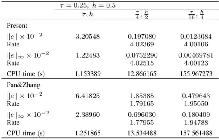
predicted fourth–order rate of convergence. We can also say that when we use smaller time and space steps, numerical values are almost the same as exact values. The CPU time for two methods are listed in Tables III and IV. It can be seen that the computational efficiency of the present method are slightly better than that of Pan&Zhang method [15], in term of CPU time. However, the construction of the novel scheme requires only a regular five–point stencil at a higher time level, which is similar to the standard second–order Crank– Nicolson scheme and Pan&Zhang scheme [15].

As in Tables V and VI, the values of Qn _andEn _{at any}

time t ∈ [0,40], which results from the present method, coincide with the theory. The quantities Qn _{and E}n _seem

to be conserved on the average, i.e. they are contained in a small interval but there are fluctuations.

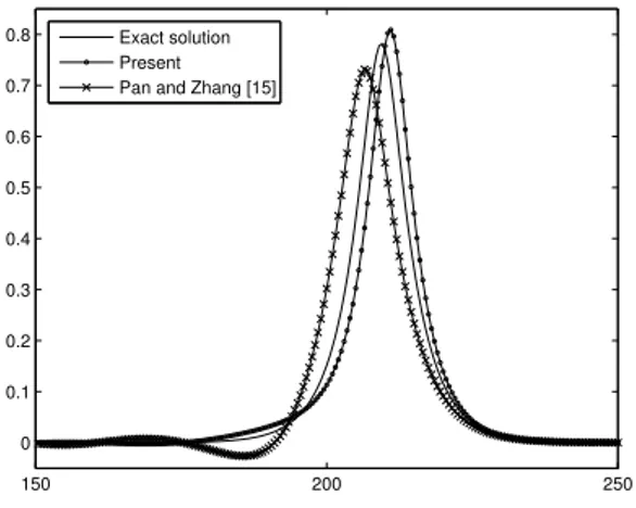
Figs. 7 and 8 show numerical solutions at t = 200with p= 4 and8. The results from the Pan&Zhang method [15] are slightly oscillate at the left side of the solitary wave in case ofp= 8. However, the results from the present method are almost perfectly sharp in both casesp= 4and8. From the point of view for the long time behavior of the resolution, the present method can be seen to be much better than the method in [15].

The solitary waves obtained by the present scheme are plotted in Figs. 9 and 10 using τ = 0.25, h = 0.5, xl = −60, xr = 200, and p = 4,8. The solitons at t = 60 and

TABLE III

RATE OFCONVERGENCE ANDCPUTIME WITHp= 4ANDt= 40.

τ= 0.25, h= 0.5

τ, h τ 4,

h 2

τ 16,

h 4

Present

kek ×10−2

3.20548 0.197080 0.0123084

Rate 4.02369 4.00106

kek∞×10 −2

1.22483 0.0752290 0.00469781

Rate 4.02515 4.00123

CPU time (s) 1.153389 12.866165 155.967273

Pan&Zhang

kek ×10−2

6.41825 1.85385 0.479643

Rate 1.79165 1.95050

kek∞×10 −2

2.38960 0.696030 0.180409

Rate 1.77955 1.94788

CPU time (s) 1.251865 13.534488 157.561488

TABLE IV

RATE OFCONVERGENCE ANDCPUTIME WITHp= 8ANDt= 40.

τ= 0.25, h= 0.5

τ, h τ4, h 2

τ 16,

h 4

Present

kek ×10−2

3.18080 0.194284 0.0121337

Rate 4.03315 4.00108

kek∞×10 −2

1.19513 0.0727869 0.00454621

Rate 4.03734 4.00094

CPU time 1.21464 13.868260 174.397644

Pan&Zhang

kek ×10−2

6.44908 1.99919 0.525426

Rate 1.68968 1.92785

kek∞×10 −2

2.35870 0.739615 0.194938

Rate 1.67314 1.92376

CPU time 1.371416 14.862871 175.068007

TABLE V DISCRETE MASSQn

.

τ= 0.25, h= 0.5

t p= 4 p= 8

t= 10 6.26580620079700 9.74208591413665

t= 20 6.26580620078861 9.74208595412127

t= 30 6.26580619948382 9.74208578472995

t= 40 6.26580617252808 9.74208558745239

Q(0) 6.26580620079328 9.74208618205024

TABLE VI DISCRETE ENERGYEn

.

τ= 0.25, h= 0.5

t p= 4 p= 8

t= 10 2.86723006370139 4.73479863443071

t= 20 2.86725271321602 4.73481771538282

t= 30 2.86726739317968 4.73483391314363

t= 40 2.86727839480750 4.73485101919594

E(0) 2.86718872840474 4.73477831492679

120 agree with the soliton at t = 0 quite well, which also shows the accuracy of the scheme.

VI. CONCLUSIONS

200 210 220 230 240 250 0

0.1 0.2 0.3 0.4 0.5 0.6 0.7

Exact solution Present Pan and Zhang [15]

Fig. 7. Numerical solutions atp = 4, xl=−60, xr = 300, h= 0.5,

τ=h2

, andt= 200.

150 200 250

0 0.1 0.2 0.3 0.4 0.5 0.6 0.7

0.8 Exact solution Present Pan and Zhang [15]

Fig. 8. Numerical solutions atp = 8, xl=−60, xr = 300, h= 0.5,

τ=h2

, andt= 200.

−50 0 50 100 150 200

−0.1 0 0.1 0.2 0.3 0.4 0.5 0.6 0.7

t = 0 t = 60 t = 120

Fig. 9. Numerical solutions atp= 4.

addition, the numerical experiments show that the present method supports the analysis of convergence rate.

It is obvious from numerical experiments that the present method, the scheme (9)–(11), gives the well resolution for the Rosenau–RLW equation. It is possible that the solitary wave obtained by this novel method can be smoothed out, at long time, by type of the high–order accuracy.

ACKNOWLEDGMENT

This research was supported by Chiang Mai University.

−50 0 50 100 150 200

−0.1 0 0.1 0.2 0.3 0.4 0.5 0.6 0.7 0.8

t = 0 t = 60 t = 120

Fig. 10. Numerical solutions atp= 8.

REFERENCES

[1] K. Mohammed, “New Exact Travelling Wave Solutions of the (3+1) Dimensional Kadomtsev–Petviashvili (KP) Equation,”IAENG Interna-tional Jounal of Applied Mathematics, vol. 37, no. 1, pp. 17–19, 2007. [2] J.V. Lambers, “An Explicit, Stable, High–Order spectral Method for the Wave Equation Based on Block Gaussian Quadrature,” IAENG International Jounal of Applied Mathematics, vol. 38, no. 4, pp. 233– 248, 2008.

[3] JC Chen and W. Chen, “Two–Dimensional Nonlinear Wave Dynamics in Blasius Boundary Layer Flow Using Combined Compact Difference Methood,”IAENG International Jounal of Applied Mathematics, vol. 41, no. 2, pp. 162–171, 2011.

[4] A.R. Bahadir, “Exponential Finite–Difference Method Applied to Korteweg–de Vries Equation for Small Times,”Applied Mathematics and Computation, vol. 160, no. 3, pp. 675–682, 2005.

[5] S. Ozer and S. Kutluay, “An Analytical–Numerical Method Applied to Korteweg–de Vries Equation,”Applied Mathematics and Computation, vol. 164, no. 3, pp. 789–797, 2005.

[6] Y. Cui and D.-k. Mao, “Numerical Method Satisfying the First Two Conservation Laws for the Korteweg–de Vries Equation,”Journal of Computational Physics, vol. 227, pp. 376–399, 2007.

[7] D.H. Peregrine, “Calculations of the Development of an Undular Bore,”

Journal of Fluid Mechanics, vol. 25, pp. 321–330, 1996.

[8] D.H. Peregrine, “Long Waves on a Beach,”Journal of Fluid Mechanics, vol. 27, pp. 815–827, 1997.

[9] P. Rosenau, “A Quasi–Continuous Description of a Nonlinear Trans-mission Line,”Physica Scripta, vol. 34, pp. 827–829, 1986.

[10] P. Rosenau, “ Dynamics of Dense Discrete Systems,” Progress of Theoretical Physics, vol. 79, pp. 1028–1042, 1988.

[11] M.A. Park, “On the Rosenau Equation,” Mathematica Aplicada e Computacional, vol. 9, no. 2, pp. 145–152, 1990.

[12] M.A. Park, “Pointwise Decay Estimate of Solutions of the Generalized Rosenau Equation,”Journal of the Korean Mathematical Society, vol. 29, pp. 261–280, 1992.

[13] J.-M. Zuo, Y.-M. Zhang, T.-D. Zhang, and F. Chang, “A New Con-servative Difference Scheme for the General Rosenau–RLW Equation,”

Boundary Value Problems, vol. 2010, Article ID 516260, 13 pages, 2010.

[14] X. Pan and L. Zhang, “On the Convergence of a Conservative Numerical Scheme for the Usual Rosenau–RLW Equation,” Applied Mathematical Modelling, vol. 36, pp. 3371–3378, 2012.

[15] X. Pan and L. Zhang, “Numerical Simulation for General Rosenau– RLW Equation: An Average Linearized Conservative Scheme,” Mathe-matical Problems in Engineering, vol. 2012, Article I517818, 15 pages, 2012.

[16] X. Pan, K. Zheng, and L. Zhang, “ Finite Difference Discretization of the Rosenau–RLW Equation,”Applicable Analysis, vol. 92, no. 12, pp. 2578–2589, 2013.

[17] N. Atouani and K. Omrani, “Galerkin Finite Element Method for the Rosenau–RLW Equation,”Computers and Mathermatics with Applica-tions, vol. 66, pp. 289–303, 2013.

[18] R.C. Mittal and R.K. Jain, “ Numerical Solution of General Rosenau– RLW Equation Using Quintic B–Splines Collocation Method,” Com-munication in Numerical Analysis, vol. 2012, Article ID cna-00129, 16 pages, 2012.

[20] F.E. Ham, F.S. Lien, and A.B. Strong, “A Fully Conservative Second– Order Finite Difference Scheme for Incompressible Flow on Nonuni-form Grids,”Journal of Computational Physics, vol. 177, pp. 117–133, 2002.