Dynamic Adjustment of Climatological Ozone Boundary Conditions for Air-Quality Forecasts

(1)

ACPD

10, 13643–13688, 2010

Dynamic Adjustment of Climatological Ozone Boundary

Conditions

P. A. Makar et al.

Title Page

Abstract Introduction

Conclusions References

Tables Figures

◭ ◮

Back Close

Full Screen / Esc

Printer-friendly Version Interactive Discussion

Discussion

P

a

per

|

Dis

cussion

P

a

per

|

Discussion

P

a

per

|

Discussio

n

P

a

per

Atmos. Chem. Phys. Discuss., 10, 13643–13688, 2010 www.atmos-chem-phys-discuss.net/10/13643/2010/ doi:10.5194/acpd-10-13643-2010

Atmospheric Chemistry and Physics Discussions

This discussion paper is/has been under review for the journal Atmospheric Chemistry and Physics (ACP). Please refer to the corresponding final paper in ACP if available.

Dynamic Adjustment of Climatological

Ozone Boundary Conditions for

Air-Quality Forecasts

P. A. Makar1, W. Gong1, C. Mooney2, J. Zhang1, D. Davignon3, M. Samaali3, M. D. Moran1, H. He1, D. W. Tarasick1, D. Sills4, and J. Chen3

1

Air Quality Research Division, Science and Technology Branch, Environment Canada, 4905 Dufferin Street, Toronto, Ontario, M3H 5T4, Canada

2

Air Quality Science Unit, Environment Canada, Edmonton, Alberta, Canada

3

Air Quality Modelling Applications Section, Environment Canada, 2121 TransCanada Highway, Dorval, Quebec, H9P 1J3, Canada

4

National Laboratory for Nowcasting and Remote Sensing Meteorology, Environment Canada, 4905 Dufferin Street, Toronto, Ontario, Canada

Received: 3 May 2010 – Accepted: 5 May 2010 – Published: 1 June 2010 Correspondence to: P. A. Makar (paul.makar@ec.gc.ca)

(2)

ACPD

10, 13643–13688, 2010

Conditions

P. A. Makar et al.

Title Page

Tables Figures

◭ ◮

Back Close

Full Screen / Esc

Discussion

P

a

per

|

Dis

cussion

P

a

per

|

Discussion

P

a

per

|

Discussio

n

P

a

per

|

Abstract

Ten different approaches for applying lateral and top climatological boundary conditions for ozone have been evaluated using the off-line regional air-quality model AURAMS. All ten approaches employ the same climatological ozone profiles, but differ in the manner in which they are applied, via the inclusion or exclusion of (i) a dynamic adjust-5

ment of the climatological ozone profile in response to the model-predicted tropopause height, (ii) a sponge zone for ozone on the model top, (iii) upward extrapolation of the climatological ozone profile, and (iv) different mass consistency corrections. The model performance for each approach was evaluated against North American surface ozone and ozonesonde observations from the BAQS-Met field study period in the summer of 10

2007. The original daily one-hour maximum surface ozone biases of about₊15 ppbv were greatly reduced (halved) in some simulations using alternative methodologies. However, comparisons to ozonesonde observations showed that the reduction in sur-face ozone bias sometimes came at the cost of significant positive biases in ozone concentrations in the free troposphere and upper troposphere. The best overall per-15

formance throughout the troposphere was achieved using a methodology that included dynamic tropopause height adjustment, no sponge zone at the model top, extrapolation of ozone when required above the limit of the climatology, and no mass consistency cor-rections (global mass conservation was still enforced). The simulation using this model version had a one-hour daily maximum surface ozone bias of ₊8.6 ppbv, with small 20

reductions in model correlation, and the best comparison to ozonesonde profiles. This recommended and original methodologies were compared for two further case studies: a high-resolution simulation of the BAQS-Met measurement intensive, and a study of the downwind region of the Canadian Rockies. Significant improvements were noted for the high resolution simulations during the BAQS-Met measurement intensive pe-25

(3)

ACPD

10, 13643–13688, 2010

Conditions

P. A. Makar et al.

Title Page

Tables Figures

◭ ◮

Back Close

Full Screen / Esc

Discussion

P

a

per

|

Dis

cussion

P

a

per

|

Discussion

P

a

per

|

Discussio

n

P

a

per

that associated with boundary layer turbulent mixing, may contribute to ozone positive biases.

1 Introduction

Regional-scale chemical transport models (CTMs) require the specification of chemical concentrations on their lateral and top boundaries, in order to accurately simulate con-5

centrations of long-lived species within the model domain (e.g. Brost, 1987). Most re-search to date on this topic has centred on boundary conditions for tropospheric ozone due both to its importance as an air pollutant and to the presence of a huge reservoir of ozone in the stratosphere. Accurate forecasting of ozone in the Los Angeles area was shown to be critically dependent on the treatment of ozone at inflow boundaries 10

for regional models studying reactive organic gas and NO_x control strategies in that area (Winner et al., 1995). Mathur et al. (2005) noted that poor regional CTM ozone performance for free tropospheric ozone could be linked to lateral boundary condition specification, as well as the model boundary layer - free troposphere exchange mech-anisms. and the chemical mechanisms used in the models. Simple boundary condition 15

treatments such as “zero-gradient”, where the spatial gradients of the chemical species are assumed to be zero on the boundaries, have been shown to be inadequate, but the quality of the data used for non-zero-gradient boundary conditions is of key importance (Tarasick et al., 2007; Samaali et al., 2009). Consistent positive biases in regional model ozone simulations have also been linked to lateral boundary condition specifica-20

tion (Yu et al., 2007). In the latter study, the linkage between the boundary conditions and transport and diffusion was found to be critical in improving ozone predictions.

Model performance is considerably improved with the use of time-invariant chem-ical lateral boundary conditions based on observations, compared to zero-gradient boundary conditions (Samaali et al., 2009). A comparison of regional CTM simula-25

(4)

ACPD

10, 13643–13688, 2010

Conditions

P. A. Makar et al.

Title Page

Tables Figures

◭ ◮

Back Close

Full Screen / Esc

Discussion

P

a

per

|

Dis

cussion

P

a

per

|

Discussion

P

a

per

|

Discussio

n

P

a

per

|

compared for the Southern Oxidants Study (Song et al., 2008). The use of the bound-ary conditions provided by the global model improved the regional CTM’s predictions of both diurnal variations and daily maxima of surface ozone concentrations relative to time-invariant, fixed boundary conditions. The global-model-derived boundary con-ditions also gave better agreement with the observed vertical structure in the middle 5

and upper troposphere. Model simulations using lateral boundary conditions derived from time-invariant sources, global air pollution model simulations, and time-varying ozonesonde data have been compared to observations (Tang et al., 2007, 2009). Correlation coefficients improved with the use of the global CTM output as regional model boundary conditions, but positive mean biases also increased for some of the 10

global models employed, whereas the boundary conditions derived from ozoneson-des improved the upper Troposphere ozone correlations. Upper troposphere negative ozone biases such as noted by Tarasick et al.(2007) have been decreased in magni-tude through the use of lateral boundary conditions provided by global CTMs (Mena-Carrasco et al., 2007). European regional ozone simulations comparing the use of 15

climatological ozone profiles versus time-dependent profiles supplied by global CTM simulations showed a slight improvement in correlation with the use of the latter, but no significant impact on the magnitude of surface ozone peaks, which were found to result from surface ozone chemistry (Szopa et al., 2009). Ozone lateral boundary con-ditions were found to have a crucial e_ffect on surface level “background concentrations” 20

of ozone, in the same study. Similarly, van Loon et al. (2007) compared seven different regional CTMs, and found that all tended to overestimate daytime ozone concentra-tions, moreover, for one CTM of the ensemble this was the result of a systematic bias in its ozone boundary conditions. The inclusion of day and nighttime variation in ozone lateral boundary conditions has been shown to improve regional model performance 25

(Chen et al., 2003).

(5)

ACPD

10, 13643–13688, 2010

Conditions

P. A. Makar et al.

Title Page

Tables Figures

◭ ◮

Back Close

Full Screen / Esc

Discussion

P

a

per

|

Dis

cussion

P

a

per

|

Discussion

P

a

per

|

Discussio

n

P

a

per

affected the predicted mean (Tang et al., 2007). The use of zero-flux conditions at the top boundary was found to result in a significant negative ozone bias in the up-per troposphere due to the resulting exclusion of stratosphere-troposphere exchange events (Tong and Mauzerall, 2006). Such events inject stratospheric ozone into the upper troposphere episodically (cf. Holton et al., 1995; Stohl et al., 2003). Thouret et 5

al. (2006) found that the location of the tropopause was a useful indicator in order to remove synoptic and seasonal variations from ozone climatologies.

An analysis of initial and boundary conditions for ozone simulations of the northeast-ern Iberian Peninsula has shown that the impact of ozone initial conditions lasts a few days, whereas the impact of ozone boundary conditions remains important throughout 10

a simulation, particularly in regions in which the ozone precursors are dominated by short-to-medium-range transport (Jimenez et al., 2007).

In the current work, we examine the impact on tropospheric ozone forecasts of ten di_fferent model configurations. We introduce a new methodology, dynamic tropopause height adjustment, for the use of climatology-based ozone data as regional CTM lat-15

eral and top ozone boundary conditions. This methodology uses tropopause-height forecasts at inflow boundaries to perform time-dependent adjustments of the climato-logical ozone profiles prior to their use as boundary conditions. Tests are performed for three cases; continental scale for North America for the summer of 2007 (BAQS-Met monitoring period), at high resolution in Southern Ontario during the BAQS-Met field 20

intensive (cf. Makar et al., 2007), and for a region east of the Canadian Rocky Moun-tains during the summer of 2002. The tropopause-height-based dynamic adjustment allows a regional CTM to capture some of the variability of the upper troposphere at the inflow boundaries, and results in significant improvements in both upper and surface ozone simulations, relative to observations.

(6)

ACPD

10, 13643–13688, 2010

Conditions

P. A. Makar et al.

Title Page

Tables Figures

◭ ◮

Back Close

Full Screen / Esc

Discussion

P

a

per

|

Dis

cussion

P

a

per

|

Discussion

P

a

per

|

Discussio

n

P

a

per

|

2 Methodology

2.1 Modelling System Description

AURAMS (A Unified Regional Air-quality Modelling System, version 1.4.0) consists of three main components: (a) a prognostic meteorological model, GEM (Global Envi-ronmental Multiscale model: C ˆot ´e et al., 1998); (b) an emissions processing system, 5

SMOKE (Sparse Matrix Operator Kernel Emissions: Houyoux et al., 2000; CEP, 2003); and (c) an off-line regional chemical transport model, the AURAMS Chemical Transport Model (CTM: cf. Gong et al., 2006, Cho et al., 2009, Makar et al., 2009, Smyth et al., 2009).

For the simulations of the Border Air-Quality – Meteorology (BAQS-Met) study pe-10

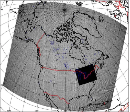
riod (Makar et al., 2010), GEM version 3.2.2 with physics version 4.5 was run on two domains: a variable-resolution, global, horizontal rotated latitude-longitude grid with a uniform core grid covering North America (575×641 grid points over the globe, with

432×565 grid points over North America, 0.1375◦or approximately 15.3 km grid

spac-ing in the core region, 450 s time step), and a local domain coverspac-ing the Great Lakes 15

area (565×494 grid points, 0.0225◦ or approximately 2.5 km grid spacing, 60 s time

step). The coarse resolution domain output was used to provide boundary conditions for the high resolution domain meteorological simulations (Fig. 1). The global variable-resolution configuration of GEM was constrained by operational analyses at six hour intervals.

20

A three level grid nesting setup was used for the AURAMS CTM simulations: an outer, 42 km polar-stereographic gird, which covered a North American domain (150×106 grid points) and used a 15 min time-step drove a smaller 15 km grid that

covered an Eastern North American domain (160×210 grid points) and used a fifteen

minute time-step; this second grid in turn drove a third, 2.5 km grid that spanned a 25

southern Ontario domain (157×211 grid points) and used a 2-min time-step (Fig. 2).

(7)

ACPD

10, 13643–13688, 2010

Conditions

P. A. Makar et al.

Title Page

Tables Figures

◭ ◮

Back Close

Full Screen / Esc

Discussion

P

a

per

|

Dis

cussion

P

a

per

|

Discussion

P

a

per

|

Discussio

n

P

a

per

as lateral boundary conditions for the two nested domains. Upper boundary condition methodologies were applied for all AURAMS domains.

2.2 Variations on a theme: ten methodologies

In our Base Case (original AURAMS configuration), the lateral and top boundary con-ditions for ozone were extracted from a global, monthly-varying gridded ozone clima-5

tology developed by Logan (1999). The US standard atmosphere was used to map ozone profiles at different locations from the pressure levels used by the climatology onto model vertical levels; and ozone values above the 100 mb top of the climatology were assumed to remain constant with height. The ten scenarios carried out here use same modelling structure (described above) for each simulation. The differences 10

between the scenarios relate to four different factors:

(a) Dynamic tropopause-height adjustment. This methodology still makes use of the

Logan (1999) ozone climatology in generarting boundary conditions, but the manner in which the climatology is applied differs from the standard treatment in AURAMS. The concept arises from examining an intensive series of twice-daily ozonesonde ob-15

servations made in southwestern Ontario during the summer 2007 BAQS-Met field study, which suggest that the ozone profiles taken during short-lived stratosphere-troposphere exchange events di_ffer from those representative of background condi-tions (He et al., 2010). During one of these events, ozone in the middle to upper tro-posphere may be increased by hundreds of ppbv and may be a factor of four or more 20

higher than typical values in the upper troposphere. The climatological ozone vertical profiles that are used in most limited-area regional air-quality models to specify bound-ary conditions, however, are long-term averages. At an upper tropospheric level close to the climatological tropopause level, the time average will thus include “typical” upper-tropospheric ozone concentrations (when the actual tropopause is located at or above 25

(8)

ACPD

10, 13643–13688, 2010

Conditions

P. A. Makar et al.

Title Page

Tables Figures

◭ ◮

Back Close

Full Screen / Esc

Discussion

P

a

per

|

Dis

cussion

P

a

per

|

Discussion

P

a

per

|

Discussio

n

P

a

per

|

exchange (STE) events. The average will thus be considerably altered (increased) by day-to-day variations in tropopause height and by sporadic cross-tropopause events (Thouret et al., 2006). As a consequence, the middle to upper tropospheric ozone in the climatology will in general be higher than actual middle to upper tropospheric ozone concentrations. Moreover, if the model predicts a tropopause height that is 5

higher than the climatological one, then a stratospheric values of ozone will be applied to that part of the upper troposphere that is above the climatological tropopause. That higher ozone concentration air will then be available to be mixed downwards; in effect an artificial STE event will have been generated by the model. The use of a non-tropopause-referenced ozone climatology may thus result in positive ozone biases in 10

the upper troposphere.

In order to test this hypothesis, a relatively simple approach was used to modify the existing boundary conditions. Four observation-based concepts were used in devising the procedure.

First, the observation was made that the height of the tropopause as indicated by 15

temperature profiles was closely linked to the ozone profile. Both fields show rapid increases in magnitude with increasing height above the tropopause (note that the air-quality model top in this case is well below the maximum in the ozone concentrations, which occurs at greater altitudes).

Second, we noted that the inclusion of STE events will smoothed both the tempera-20

ture and ozone climatology in a similar way, relative to the background profile. A com-parison of the “US Standard Atmosphere” temperature profile to profiles in Logan’s data showed a good correspondence: both show a relatively smooth increase in magnitude rather than the sharp transition of individual background (non-exchange event) days. The US Standard Atmosphere’s tropopause height was therefore used here to repre-25

(9)

ACPD

10, 13643–13688, 2010

Conditions

P. A. Makar et al.

Title Page

Tables Figures

◭ ◮

Back Close

Full Screen / Esc

Discussion

P

a

per

|

Dis

cussion

P

a

per

|

Discussion

P

a

per

|

Discussio

n

P

a

per

et al., 2006), and in the creation of seasonal average ozone climatologies (Thouret et al., 2006).

Third, we note that the tropopause height may be estimated according to the revised World Meteorological Organization criterion, specifically (JPL, 2010):

1. “The first tropopause (i.e., the conventional tropopause) is defined as the low-5

est level at which the lapse rate decreases to 2 K km−1 _{or less, and the average}

lapse rate from this level to any level within the next higher 2 km does not exceed 2 K km−1_{(WMO, 1966).}

2. If above the first tropopause the average lapse rate between any level and all higher levels within 1 km exceed 3 K km−1_{, then a second tropopause is defined}

10

by the same criterion as under the statement above. This tropopause may be either within or above the 1 km layer (Roe and Jasperson, 1980).

3. A level otherwise satisfying the above definition of tropopause, but occuring at an altitude below that of the 500 mb level, will not be designated a tropopause unless it is the only level satisfying the definition and the average lapse rate fails 15

to exceed 3 K km−1 _{over at least 1 km in any higher layer (Roe and Jasperson,}

1980).”

Fourth and last, we noted that vertically stretching or shrinking the climatological ozone vertical profile by the ratio of tropopause heights (model-generated to US Standard at-mosphere), resulted in climatological ozone profiles that were much closer in appear-20

ance to the observed profiles in the model domain.

Two different approaches were taken to make use of these observation-based con-cepts: in the first, the ratio of the tropopause height locations (time-varying model to US Standard Atmosphere) was used to linearly scale all ozone climatology heights (“dynamic” scaling: DYN1, see Table 1), prior to their application on the lateral and top 25

(10)

ACPD

10, 13643–13688, 2010

Conditions

P. A. Makar et al.

Title Page

Tables Figures

◭ ◮

Back Close

Full Screen / Esc

Discussion

P

a

per

|

Dis

cussion

P

a

per

|

Discussion

P

a

per

|

Discussio

n

P

a

per

|

above and below the tropopause respectively, to scale the heights of the ozone clima-tology (DYN2, see Table 1). Both of these approaches dynamically shift the location of the ozone climatological fields in the vertical, prior to their use as model boundary conditions at any given time step.

(b) Extrapolation of the available ozone climatology to (or beyond) the model top.

5

The default AURAMS 1.4.0 makes use of the static ozone climatology of Logan (1999), the top layer of which is at 100 mb. This climatological top level was often below the modified Gal-Chen coordinate AURAMS top of 18 km: by default, AURAMS would use the uppermost climatological ozone value for all grid points above the 100 mb region. The (Extrap) and (Extrap2) methodologies extrapolate from the existing climatology 10

above that level, either internally to the model at every gridpoint requiring extrapolation (Extrap), or using a pre-processing step of extrapolating all climatological ozone values to 50 mb (well above the AURAMS model top, then interpolating within the resulting 50 to 100 mb region within the model, Extrap2). Both methodologies attempt to make the model’s use of the upper portion of the available climatology more realistic (since 15

the ozone profile is known to continue increasing above 100 mb); a better, longer-term solution would be to generate new climatology from available data, that always extends above the AURAMS top.

(c) The use or absence of a sponge zone at the model lid.Sponge zones are

some-times employed to smooth the transported field in the vicinity of a static boundary 20

condition, to prevent spatial discontinuities between the boundary condition and the time-dependent fields from resulting in errors (e.g. from over- and under-shooting in Semi-Lagrangian advection). However, the use of a sponge zone in a region with a large gradient in concentration (as is the case for ozone, at the model top) may de facto increase the transport of upper boundary ozone into the model domain. The sponge 25

(11)

ACPD

10, 13643–13688, 2010

Conditions

P. A. Makar et al.

Title Page

Tables Figures

◭ ◮

Back Close

Full Screen / Esc

Discussion

P

a

per

|

Dis

cussion

P

a

per

|

Discussion

P

a

per

|

Discussio

n

P

a

per

of the last time-step’s forecast and the climatology, and the 3rd layer down being com-pletely determined by the forecast. The very coarse vertical resolution near the top of the model (∼3 km) implies that errors of this nature associated with the sponge zone

may be substantial. One set of tests (Wosp; “without sponge”) evaluates the effect of removing this sponge zone.

5

(d) The choice of mass consistency correction methodology. The meteorological

model does not formally conserve air density in its prognostic equations, and interpola-tion errors in the wind fields resulting from interpolainterpola-tion between meteorological model and air-pollution model grids will also occur. The consistency between wind fields and air density may be reduced by these considerations; previous work (Byun, 1999a,b; 10

Odman and Russell, 2000; Lee et al., 2004; Hu et al., 2006) has shown that correcting for these effects improves the accuracy of air-quality forecasts. To examine the poten-tial impact of mass consistency corrections on the transported chemical species, three di_fferent methodologies will be considered here: (1) The wind fields may be corrected – that is, the error in mass consistency is assumed to reside in one or more of the com-15

ponents of the 3D winds, and corrections to the wind field are applied in order to reduce this error (Yamartino, 1993, Byun, 1999a, b); (2) The errors in mass consistency are assumed to be reflected by errors in air density: the ratio of the meteorological model’s diagnostically predicted air density to the air density that resulting from advection from the previous time step, is used to correct the advected tracers; (3) The errors in mass 20

consistency are assumed to be reflected by errors in both air density and the vertical coordinate Jacobian transformation: the ratio of the advected product of the Jacobian and density to the diagnostically predicted product of the Jacobian and density is used to correct the advected product of the Jacobian and the tracer of interest. Four different approaches were thus compared here: no mass consistency correction (Opt1), a ver-25

tical wind field correction (Opt2), an air density advection and ratio correction (Opt3), and a product of air density with Jacobian advection and ratio correction (Opt4).

(12)

ACPD

10, 13643–13688, 2010

Conditions

P. A. Makar et al.

Title Page

Tables Figures

◭ ◮

Back Close

Full Screen / Esc

Discussion

P

a

per

|

Dis

cussion

P

a

per

|

Discussion

P

a

per

|

Discussio

n

P

a

per

|

constraints led us to examine a sub-set here. Our tests thus represent improvements and additions along a particular line of enquiry rather than an exhaustive examination of all possible combinations. Table 1 describes the individual scenarios, and gives their designators used in subsequent analysis.

Each methodology was used in a separate 2.5 month scenario simulation (subse-5

quent to two weeks spin-up) for the BAQS-Met 42 km domain (Fig. 2). The results were compared using standard statistics to surface observations from the AIRNow net-work, and to ozonesondes released at the BAQS-Met study’s Harrow site (42.03 N, 82.9 W). The base case, and the methodology deemed to have the best overall per-formance, were then used for 15 km and 2.5 km BAQS-Met simulations (only the latter 10

will be discussed here), and for a separate set of simulations at 36 and 12 km grid spacing along a domain in western Canada. The latter shows the effects of the choice of boundary conditions on ozone originating from exchange events and the importance of the coupling between boundary layer and free troposphere on the forecasted ozone concentration.

15

3 Model Performance Evaluation

3.1 North American Domain: 42 km grid BAQS-Met simulations compared to

AIRNow

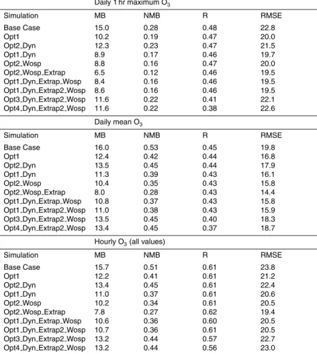
AIRNow data between 3 June 2007 and 31 August 2007 were used to evaluate each of the model scenarios described above, for the largest domain shown in Fig. 2. The 20

mean bias (MB), normalized mean bias (NMB), correlation coefficient (R), and root-mean-square-error (RMSE) were calculated for the daily 1-hr maximum, daily mean, and hourly (all values) of both ozone and PM2.5, with the results given in Tables 2 and

3, respectively.

The ozone results (Table 2) show that all methodologies have a positive mb and 25

(13)

ACPD

10, 13643–13688, 2010

Conditions

P. A. Makar et al.

Title Page

Tables Figures

◭ ◮

Back Close

Full Screen / Esc

Discussion

P

a

per

|

Dis

cussion

P

a

per

|

Discussion

P

a

per

|

Discussio

n

P

a

per

The original model setup, Base Case (Table 1), has the highest MB, NMB and RMSE of all methodologies. The Base Case also has the highest correlation coefficient for the daily 1 hour maximum and daily mean, though the variation in correlation coefficients between the different methodologies is usually small.

The simulation with the best overall performance (based on these surface obser-5

vations alone) is Opt2 Wosp Extrap; incorporating a vertical velocity wind-field mass consistency correction, no sponge zone at the model top, and climatological ozone concentrations extrapolated in instances where the model top is above the top of the climatology. This simulation has the lowest magnitude MB, NMB and RMSE, without a significant decrease in R compared to the base case (for hourly ozone, this simulation 10

has the highest R score).

A second group of methodologies (Opt1 Dyn, Opt2 Wosp, Opt1 Dyn Extrap Wosp, and Opt1 Dyn Extrap2 Wosp) have similar overall performance, worse than Opt2 Wosp Extrap, but better than the other scenarios and the Base Case. These scenarios still show a significant improvement in the MB, NMB, RMSE relative to the 15

base case, again with relatively little change in the correlation coefficient.

A final group of methodologies (Opt1, Opt2 Dyn, Opt3 Dyn Extrap2 Wosp, Opt4 Dyn Extrap2 Wosp) also have similar overall performance, and are the closest to the relatively poor performance of the original Base Case.

Comparing the above statistics, a few observations may be made: 20

1. The incorporation of dynamic tropopause improves the model prediction at the surface;

2. Removing the sponge zone also helps to reduce the positive ozone bias at the surface;

3. Extrapolating O3 climatology beyond 100 mb (as opposed to simple extension),

25

(14)

ACPD

10, 13643–13688, 2010

Conditions

P. A. Makar et al.

Title Page

Tables Figures

◭ ◮

Back Close

Full Screen / Esc

Discussion

P

a

per

|

Dis

cussion

P

a

per

|

Discussion

P

a

per

|

Discussio

n

P

a

per

|

4. Removal of the mass consistency adjustment (regardless of type) reduces the positive bias at the surface.

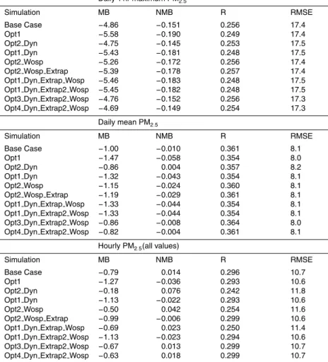
The corresponding scores for PM2.5 are shown in Table 3. The changes to the PM2.5

are relatively small compared to ozone (compare NMB columns, Tables 2 and 3); the changes in methodology have a much larger impact on ozone forecast accuracy, than 5

on that of particulate matter.

From the analysis of the surface sites, the Opt2 Wosp Extrap has the best perfor-mance, and results in the greatest improvement in MB, NMB and RMSE compared to the other scenarios. However, this setup has relatively poor performance in the mid-to-upper troposphere, as will be discussed below.

10

3.2 North American Domain: 42 km grid BAQS-Met simulations compared to

Harrow Ozonesondes

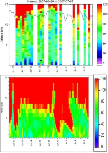
Twice daily ozonesonde measurements were carried out at the Harrow BAQS-Met site. A comparison between the Base Case ozone and the observations is shown in Fig. 3. The most striking feature about the comparison is the extent to which the 15

model ozone is biased high in the free and upper troposphere. In the observations (Fig. 3a), ozone in the region between 3 and 10 km is rarely greater than 80 ppbv, while the Base Case values (3b) are often greater than 120 ppbv, especially above 7 km. The observations show the presence of high concentration ozone resulting from troposphere/stratospheric exchange (He et al., 2010) – similar events are depicted in 20

the Base Case simulation, but are much stronger than in the observations, resulting in

>120 ppbv being brought down to within 2km of the surface, rather than the 7 to 8 km

lower reach of these intrusions depicted in the observations. The Base Case scenario is clearly biased high throughout the ozone profile, not just at the surface as suggested by Table 2.

25

(15)

ACPD

10, 13643–13688, 2010

Conditions

P. A. Makar et al.

Title Page

Tables Figures

◭ ◮

Back Close

Full Screen / Esc

Discussion

P

a

per

|

Dis

cussion

P

a

per

|

Discussion

P

a

per

|

Discussio

n

P

a

per

methodologies considered here. The surface network mean biases have been con-toured using kriging in order to better show the spatial pattern, and a mask has been applied to show only the part of the domain containing station data. These figures show that the surface performance (images on the right-hand-side of Fig. 4 and in the sum-mary statistics of Table 2) is sometimes at odds with the performance throughout the 5

profile (images on the left-hand-side of Fig. 4). The Base Case, and all of the method-ologies that donot make use of some form of dynamic ozone climatology (Fig. 4 a–d; Base Case, Opt1, Opt2 Wosp, Opt2 Wosp Extrap, Opt2) all significantly overestimate the ozone concentrations in the model profile.

The response at the surface (right-hand surface maps, Fig. 4) is varied between 10

the di_fferent simulations. For example, the “Opt2 Wosp Extrap” simulation, which had the best overall statistical scores from the above analysis (Fig. 4d), has achieved that end through the creation of negative mean bias values in much of the domain, while still being biased high through much of the middle to upper troposphere (compare simulated ozone profiles, Fig. 4d, to observations, Fig. 3a). With the exception of 15

the “density advection” and “density * Jacobian” simulations (Fig. 4 i and j, respec-tively), those simulations employing some form of dynamic ozone climatology adjust-ment have more realistic ozone profiles (Fig. 4 e–h). Those with the closest appear-ance to the measured ozone profile are Opt1 dyn, and Opt1 Dyn Extrap2 Wosp. Of these, Opt1 Dyn Extrap2 Wosp has the better surface performance, from the statistics 20

of Table 2.

Comparing different simulations in Fig. 4 allows further analysis of the different methodologies. For example, comparing the simulated ozone profiles of (4a) and (4b): an undesired result of the use of the vertical velocity mass consistency is an increase in the downward transport of ozone: ozone concentrations are higher at any given altitude 25

(16)

ACPD

10, 13643–13688, 2010

Conditions

P. A. Makar et al.

Title Page

Tables Figures

◭ ◮

Back Close

Full Screen / Esc

Discussion

P

a

per

|

Dis

cussion

P

a

per

|

Discussion

P

a

per

|

Discussio

n

P

a

per

|

profile values results from the incorporation of a dynamic ozone climatology methodol-ogy (compare 4a with 4e, or 4f with 4b), though high concentration ozone is still mixed down to the surface. If the mass consistency correction on the vertical velocities is then removed, an ozone profile similar to the observations results (compare 4e and 4f). Fig-ures 4(g) and (4h) are variations on this latter theme; no mass consistency correction, 5

but without the top sponge zone, with different methods of doing the extrapolation, re-sulting in only minor changes to both profiles and surface statistics. Mass consistency is again explored in Figs. (4i and j). Here, the density and density*Jacobian advec-tion methodologies were applied, but these reduce the overall accuracy of the results; high ozone concentrations are again brought down from upper levels. Note that these 10

two di_fferent approaches resulted in similar surface statistics, yet very di_fferent ozone profiles in the upper Troposphere.

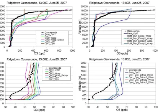
Time-specific ozone profiles are examined in more detail in Figs 5 and 6, which show the observed ozone (diamond symbols) and the simulated ozone from each of the different methodologies, throughout the entire modelled profile (a, b) and in the 15

lowest 2km of the atmosphere (c, d). Figure 5 shows the behaviour when the ozone is perturbed by a stratospheric exchange event, while Fig. 6 depicts the more typical behaviour in the absence of intrusions. Figs 5a and 6a show that the best surface-performance scenario (Opt2 Wosp Extrap) is biased very high above 6 km altitude. The methodologies with the best fit to the observations up to 12 km all incorporate 20

dynamic ozone climatology (Figs. 5 and 6, a, b). Figures 5 and 6 (c, d) show that the choice of boundary condition methodologies has a strong impact on the model results close to the surface; the shape of the simulated profiles and their proximity to the observations vary by 20 ppbv when the profile is perturbed by the exchange event (5c, d), and 12 ppbv under more “normal” conditions (6c, d). The simulation with the 25

best fit at thesurface(Opt2 Wosp Extrap, here, 5c, 6c), tends to be biased high in the middle to upper troposphere.

(17)

ACPD

10, 13643–13688, 2010

Conditions

P. A. Makar et al.

Title Page

Tables Figures

◭ ◮

Back Close

Full Screen / Esc

Discussion

P

a

per

|

Dis

cussion

P

a

per

|

Discussion

P

a

per

|

Discussio

n

P

a

per

through the use of dynamic ozone climatology, no sponge zone at the model top, ex-trapolation of the existing climatology to 50 mb, and no mass consistency correction in the wind fields (methodology Opt1 Dyn Extrap2 Wosp). Two further analyses of case studies follow, comparing this recommended methodology to the Base Case, at higher resolution.

5

4 Case Study 1: AURAMS high resolution simulations compared to BAQS-Met

Mesonet surface observations

This case study examines the impact of improved model forecasts at coarse resolution (transferred to the high resolution domain as lateral boundary conditions) on the model forecast at the nested higher resolution, as well as that of the top boundary condition, 10

applied at all resolutions. The Base Case and Opt1 Dyn Extrap2 Wosp 42 km simula-tions were used to provide the lateral boundary condisimula-tions for 15km and thence 2.5km simulations (domains shown in Fig. 2). The top boundary condition within all three domains made use of the Base Case or Opt1 Dyn Extrap2 Wosp methodologies. Sur-face ozone measurements (5 min sampling), obtained using a local mesonet during 15

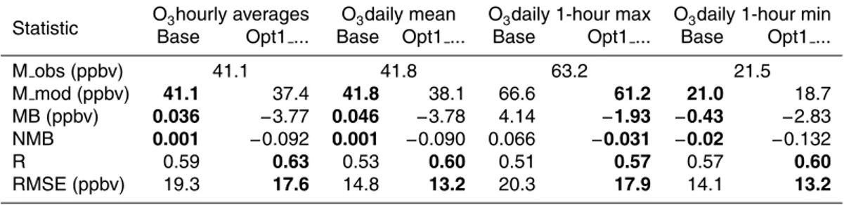
the BAQS-Met study, were averaged to hourly values (Fig. 7). The surface ozone concentrations in the study region are strongly a_ffected by lake- and land-breeze cir-culations (Makar et al., 2010): the summary statistics for the two runs are compared here to determine the relative impact of the modified boundary conditions (indirectly, through transfer on the lateral boundary, and directly, through the top boundary) on 20

the very local ozone predictions. Table 4 summarizes the comparison for the different metrics and statistical measures. Bold-face numbers within the table identify which of the two high resolution simulations (Base Case or Opt1 Dyn Extrap2 Wosp) had the better score. For this small subdomain, the original Base Case had better mb and NMB scores for the hourly average ozone, the daily mean ozone, and the daily 1 hour 25

(18)

ACPD

10, 13643–13688, 2010

Conditions

P. A. Makar et al.

Title Page

Tables Figures

◭ ◮

Back Close

Full Screen / Esc

Discussion

P

a

per

|

Dis

cussion

P

a

per

|

Discussion

P

a

per

|

Discussio

n

P

a

per

|

scenario outperformed the Base Case for all metrics. These results show that the choice of ozone climatology methodology can have a significant impact even at the local scale (through the lateral transfer from lower-resolution domains, and through the top boundary condition). From the forecasting standpoint, accurate prediction of the maximum ozone is of key importance: the Opt1 Dyn Extrap2 Wosp scenario signifi-5

cantly improves the model results, relative to the Base Case.

Figure 8 shows example ozone time series from the Bear Creek site (42.54 N, 82.39 W); the improvement to the magnitude of the peak values and the overall fit to the observations being noticeable in both examples.

5 Case Study 2: AURAMS simulations over the Rockies Compared to local

10

Mesonet, summer 2002

This second case study was chosen to analyse the persistent positive bias just east of the Canadian Rockies noticeable in the kriged mean bias surfaces in all of the sim-ulations of Fig. 4. This region is of particular interest from the standpoint of ozone forecasting in Canada, due to the known occurrence of stratosphere/troposphere ex-15

change events in the measurement record (cf. Chung and Dann, 1985). The period simulated was 8 June to 31 August 2002, and the 36 km and 12 km domains used in the simulations are shown in Fig. 9. These simulations made use of GEM version 3.2.0 (353×415 grid points over the globe, with 270×353 grid points over North America,

0.22◦ _{or approximately 24 km grid spacing in the core region, 450 s time step) to}

pro-20

vide the driving meteorology. The same version of AURAMS as the previous tests was used. The 24 km GEM meteorology was used to drive both the 36 (80×105 grid points)

and the 12 km (75×115 gridpoints) AURAMS simulations.

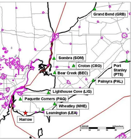
Figure 10 shows the locations of the 23 surface mesonet observation sites used for statistical evaluation, and an ozonesonde release site. The analysis which follows is 25

(19)

ACPD

10, 13643–13688, 2010

Conditions

P. A. Makar et al.

Title Page

Tables Figures

◭ ◮

Back Close

Full Screen / Esc

Discussion

P

a

per

|

Dis

cussion

P

a

per

|

Discussion

P

a

per

|

Discussio

n

P

a

per

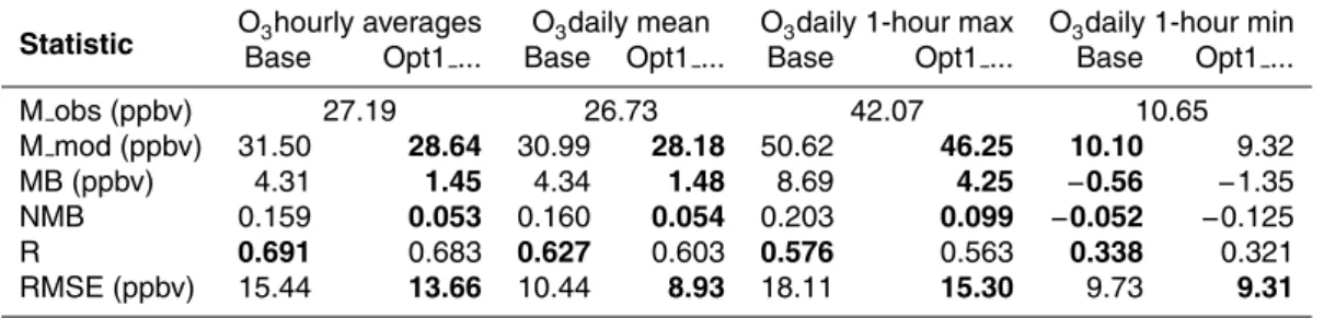
Table 5 shows the comparison results for the same statistical quantities as Table 4 for this second case study. Both simulations have positive mean biases, normalized mean biases, and root mean square errors, but these are greatly reduced in the Opt1 Dyn Extrap2 Wosp scenario compared to the base case. Mean biases and nor-malized mean biases are reduced by more than a factor of two, and RMSE values 5

are reduced by more than 1.5 ppbv, for all metrics. Correlation coefficients have de-creased slightly with the use of the new dynamic boundary condition. As in the simu-lations examined in the previous sections, the adoption of the new boundary condition methodology significantly improves the model performance.

Figure 11 compares the kriged daily 1-h surface maximum ozone mean bias values 10

between the two simulations. The use of the Opt1 Dyn Extrap2 Wosp boundary con-ditions (Fig. 11b) reduces the overall negative bias relative to the base case (Fig. 11a), though positive bias regions remain. These regions, like those for the simulations shown earlier (see Fig. 4h), are centered on major industrial areas (from south-west to north-east these are the cities of Calgary, Red Deer, Edmonton, and the Oil Sands 15

(see Fig. 10 for locations), suggesting that at least part of the remaining biases may be the result of errors in the anthropogenic ozone formation processes, as opposed to boundary condition-dominated causes.

Figure 12a compares modelled and measured surface ozone concentrations at the Edmonton East station during a series of high ozone days between 9 and 15 July. Over-20

all, the new methodology gives a closer fit to the observations, though the maximum during the time period (11 July) was better simulated by the Base Case.

An examination of the time series at different monitoring stations suggested that one troposphere/stratosphere mixing event may be responsible for part of the remaining positive biases in both simulations. Figure 12b compares the observations and the two 25

(20)

ACPD

10, 13643–13688, 2010

Conditions

P. A. Makar et al.

Title Page

Tables Figures

◭ ◮

Back Close

Full Screen / Esc

Discussion

P

a

per

|

Dis

cussion

P

a

per

|

Discussion

P

a

per

|

Discussio

n

P

a

per

|

from as high as 10 000 m to the surface, over central Alberta, northern Alberta, and Saskatchewan. This first stage resulted in 150 to 200 ppbv ozone at the 3000m above ground level. The second stage was the creation of a deep surface-based unstable planetary boundary layer (due to daytime heating), behind the passing upper low. The turbulent mixing associated with this second stage allowed the model-simulated ozone 5

to reach the surface. This final stage of the transport has a strong diurnal trend, with mixing to the surface ceasing in the evening. Tephigrams, derived from rawinsondes launched at the Stony Plain site west of Edmonton (Fig. 10, star symbol) confirm the presence of the deep well-mixed layer up to 3200 m on the 12th and 13th, but this weak-ened to 2200 m on the 14th. Observed and simulated ozonesonde values at Stony 10

Plain (Fig. 13) show the presence of high concentration ozone at 6000 m. Both simula-tions are biased low above 5500 m, the base-case has positive biases below 5500 m, while the Opt1 Dyn Extrap2 Wosp simulation has lower positive or negative biases be-low 5500 m. The location of the observed mid-troposphere ozone peak in the profile associated with the event at 5800 m is well predicted by the Opt1 Dyn Extrap2 Wsop 15

methodology, but its magnitude is biased low for both simulations. Given the nega-tive biases in the upper free troposphere, the remaining model posinega-tive biases at the surface during this event are thus likely due to the simulated boundary layer being less stable than the ambient atmosphere, on the 14th and 15th of June. The event illustrates the importance of the timing and strength of the coupling of upper level and lower level 20

ozone transport to the middle Troposphere, during STE events.

6 Discussion and conclusions

Our analysis shows that considerable improvements in model ozone simulation ac-curacy may be achieved in regional air-quality models from a careful choice of the methodology used to specify lateral and top boundary conditions from ozone clima-25

(21)

ACPD

10, 13643–13688, 2010

Conditions

P. A. Makar et al.

Title Page

Tables Figures

◭ ◮

Back Close

Full Screen / Esc

Discussion

P

a

per

|

Dis

cussion

P

a

per

|

Discussion

P

a

per

|

Discussio

n

P

a

per

and by removing mass consistency corrections. Using extrapolation to extend the ozone climatology in the vertical also improved the fit to observations in the top part of the model domain. The improvements of this overall methodology were significant, particularly in the reduction of mean biases and RMSE for the lower resolution sim-ulations, and improving correlation coefficients and RMSE at higher resolutions (and 5

for all statistical measures, at high resolution). Examination of a case study along the Rocky Mountains has suggested that the degree of coupling between the planetary boundary layer and the free troposphere is a key factor in determining the extent to which stratosphere-origin ozone is brought to the surface.

It should be noted that other combinations and permutations of methodologies tested 10

here are possible, and the impact of an individual component of a combined method-ology will vary for different levels of the atmosphere.

One surprising outcome of the work was that all three of the mass consistency cor-rections examined, resulted in excessive downward transport of ozone downwards from the upper part of the model. The best model performance for surface ozone 15

resulted from the use of a methodology combining a vertical velocity mass consistency correction, the absence of sponge zone at the model top, and extrapolation of the ozone climatology above 100 mb. However, the comparison to BAQS-Met ozoneson-des showed that this improved performance at the surface came at the expense of large positive biases in ozone concentrations in the middle to upper troposphere. It 20

is important to note that at least some of these results may depend on the particu-lar combination of meteorological model and CTM grids and grid projections, as well as their respective vertical coordinates and resolutions, the advection algorithm em-ployed, and the height of the model top. AURAMS has relatively low resolution in the vicinity of the model top compared to the driving meteorological model (GEM); this 25

(22)

ACPD

10, 13643–13688, 2010

Conditions

P. A. Makar et al.

Title Page

Tables Figures

◭ ◮

Back Close

Full Screen / Esc

Discussion

P

a

per

|

Dis

cussion

P

a

per

|

Discussion

P

a

per

|

Discussio

n

P

a

per

|

transport related to mass consistency. AURAMS makes use of a domain-wide mass conservation correction in addition to mass consistency corrections; the former may help constrain the model mass when the latter was absent. Further research is needed with coupled meteorological / air-quality models in order to determine whether diff er-ences between the meteorological and air-quality model grids used here resulted in the 5

increase in middle and upper troposphere ozone bias with the use of mass consistency corrections.

The concept of dynamic, tropopause-referenced adjustments to climatological ozone boundary conditions has been introduced here and has been shown to have a signif-icant improvement on surface ozone prediction accuracy. The algorithm used here 10

is relatively simple – future research on the specification of ozone boundary condi-tions from ozone climatologies should attempt to resolve the median and extreme-event ozone climatology, as well as the more traditional average, and consider the removal of seasonal and synoptic variations (cf. Thouret et al., 2006). The use of such improved climatological data would likely improve model performance in a similar manner to the 15

model-internal corrections shown here.

Acknowledgements. The authors would like to acknowledge the financial support of

Environ-ment Canada and the Ontario Ministry of the EnvironEnviron-ment for the BAQS-Met study. We grate-fully acknowledge the assistance of the AIRNow program and its participating stakeholders in providing near-real-time ground-level ozone observations across North America.

20

References

Berner, T., Sankey, D., and Shepherd, T. G.: The Tropopause inversion layer in models and analyses, Geophys. Res. Lett., 33, L14804, doi:10.1029/2006GL026549, 2006.

Brost, R. A.: The sensitivity to input parameters of atmospheric concentrations simulated by a regional chemical model, J. Geophys. Res., 93, 2371–2387, 1987.

25

(23)

ACPD

10, 13643–13688, 2010

Conditions

P. A. Makar et al.

Title Page

Tables Figures

◭ ◮

Back Close

Full Screen / Esc

Discussion

P

a

per

|

Dis

cussion

P

a

per

|

Discussion

P

a

per

|

Discussio

n

P

a

per

Byun, D. W.: Dynamically consistent formulations in meteorological and air quality models for multiscale atmospheric studies. Part II: mass conservation issues, J. Atmos. Sci., 56, 3808– 3820, 1999b.

CEP, 2003: Carolina Environmental Program, Sparse Matrix Operator Kernel Emission (SMOKE) modelling system, University of North Carolina, Carolina Environmental Programs,

5

Chapel Hill, NC, see http://www.smoke-model.org/index.cfm.

Chen, K. S., Ho, Y. T., Lai, C. H., and Chou, Y.-M.: Photochemical modeling and analysis of meteorological parameters during ozone episodes in Kaohsiung, Taiwan, Atmos. Environ., 37(13), 1811–1823, 2003.

Cho, S., Makar, P. A., Lee, W. S., Herage, T., Liggio, J., Li, S. M., Wiens, B., and Graham, L.:

10

Evaluation of a unified regional air-quality modeling system (AURAMS) using PrAIRie2005 field study data: The e_ffects of emissions data accuracy on particle sulphate predictions, Atmos. Environ., 43, 1864–1877, 2009.

Chung, Y. S. and Dann, T.: Observations of stratospheric ozone at the ground level in Regina, Canada, Atmos. Environ., 19, 157–162, 1985.

15

C ôt é, J., Gravel, S., M éthot, A., Patoine, A., Roch, M., and Staniforth, A.: The operational CMC-MRB Global Environmental Multiscale (GEM) model. Part 1: Design considerations and formulation, Mon. Wea. Rev., 126, 1373–1395, 1998.

Gong, W., Dastoor, A. P., Bouchet, V. S., Gong, S., Makar, P. A., Moran, M. D., Pabla, B., M ´enard, S., Crevier, L,-P., Cousineau, S., and Venkatesh, S.: Cloud processing of gases

20

and aerosols in a regional air quality model (AURAMS), Atmos. Res., 82, 248–275, 2006. He, H., Tarasick, D. W., Hocking, W. K., Carey-Smith, T.K., Rochon, Y., Zhang, J., Makar, P. A.,

Osman, M., Brook, J., Moran, M. D., Jones, D., Mihele, C., Wei, J. C., Osterman, G., Argall, P. S., McConnell, J., and Bourqui, M.: Transport analysis of ozone enhancement in southern Ontario during BAQS-Met, Atmos. Chem. Phys. Discuss., submitted, 2010.

25

Holton, J. R., Haynes, P. H., McIntyre, M. E., Douglass, A. R., Rood, R. B., and Pfister, L.: Stratosphere-troposphere exchange, Rev. Geophys., 33, 403–440, 1995.

Houyoux, M. R., Vukovich, J. M., Coats, C. J. Jr., and Wheeler, N. J. M.: Emission inventory de-velopment and processing for the Seasonal Model for Regional Air Quality (SMRAQ) project, J. Geophys. Res., 105, 9079–9090, 2000.

30

Hu, Y., Odman, M. T., and Russell, A. G.: Mass conservation in the Community Multiscale Air Quality model, Atmos. Environ., 40, 1199–1204, 2006.

(24)

ACPD

10, 13643–13688, 2010

Conditions

P. A. Makar et al.

Title Page

Tables Figures

◭ ◮

Back Close

Full Screen / Esc

Discussion

P

a

per

|

Dis

cussion

P

a

per

|

Discussion

P

a

per

|

Discussio

n

P

a

per

|

modeling in very complex terrains: A case study in the northeastern Iberian Peninsula, En-vironmental Modelling and Software, 22(9), 1294–1306, 2007.

Lee, S. M., Lee, S. M., Yoon, S. C., and Byun, D. W.: The effect of mass inconsistency of the meteorological field generated by a common meteorological model on air quality modeling, Atmos. Environ., 38, 2917–2926, 2004.

5

Logan, J. A.: An analysis of ozonesonde data for the troposphere: Recommendatioins for testing 3-D models, and development of a gridded climatology for tropospheric ozone, J. Geophys. Res., 104, 16115–16149, 1999.

Makar, P. A., Moran, M. D., Zheng, Q., Cousineau, S., Sassi, M., Duhamel, A., Besner, M., Davignon, D., Crevier, L.-P., and Bouchet, V. S.: Modelling the impacts of ammonia

10

emissions reductions on North American air quality, Atmos. Chem. Phys., 9, 7183–7212, doi:10.5194/acp-9-7183-2009, 2009.

Makar, P. A., Zhang, J., Gong, W., Stroud, C., Sills, D., Hayden, K. L., Brook, J., Levy, I., Mihele, C., Moran, M. D., Tarasick, D. W., and He., H.: Mass tracking for chemical analysis: the causes of ozone formation in southern Ontaio during BAQS-Met 2007, Atmos. Chem. Phys.

15

Discuss., in review, 2010.

Mathur, R., Shankar, U., Hanna, A. F., Odman, M. T., McHenry, J. N., Coats Jr., C. J., Alapaty, K., Xiu, A., Arunachalam, S., Olerud Jr., D. T., Byun, D. W., Schere, K. L. , Binkowski, F. S., Ching, J. K. S., Dennis, R. L., Pierce, T. E., Pleim, J. E., Roselle, S. J., Young, J. O.: Multiscale Air Quality Simulation Platform (MAQSIP): Initial applications and

per-20

formance for tropospheric ozone and particulate matter, J. Geophys. Res., 110, D13308, doi:10.1029/2004JD004918, 2005.

Mena-Carrasco, M., Tang, Y., Carmichael, G. R., Chai, T., Thongbongchoo, N., Campbell, J. E., Kulkarni, S., Horowitz, L., Vukovich, J., Avery, M., Brune, W., Dibb, J. E., Emmons, L., Flocke, F., Sachse, G. W., Tan, D., Shetter, R., Talbot, R. W., Streets, D. G., Frost, G.,

25

Blake, D.: Improving regional ozone modeling through systematic evaluation of errors using the aircraft observations during the International Consortium for Atmospheric Research on Transport and Transformation, J. Geophys. Res., 112, D12S19, doi:10.1029/2006JD007762, 2007.

Odman, M. T. and Russell, A. G.: Mass conservative coupling of non-hydrostatic meteorological

30

models with air quality models, edited by: Gryning, S.-E. and Batchvarova, E., Air Pollution Modeling and its Application XIII, Kluwer/Plenum, New York, pp. 651–660, 2000.

(25)

ACPD

10, 13643–13688, 2010

Conditions

P. A. Makar et al.

Title Page

Tables Figures

◭ ◮

Back Close

Full Screen / Esc

Discussion

P

a

per

|

Dis

cussion

P

a

per

|

Discussion

P

a

per

|

Discussio

n

P

a

per

Roe, J. M. and Jasperson: A new Tropopause definition from simultaneous ozone-temperature profiles. Interim Technical Report 1, 1 July 1979–1 July 1980, Control Data Corporation, Minneapolis Research Division, 16 pp., 1980.

Samaali, M., Moran, M. D., Bouchet, V. S., Pavlovic, R., Cousineau, S., Sassi, M.: On the influence of chemical initial and boundary conditions on annual regional air quality model

5

simulations for North America, Atmos. Environ., 43(32), 4873–4885, 2009.

Smyth, S. C., Jiang, W., Roth, H., Moran, M. D., Makar, P. A., Yang, F., Bouchet, V. S., and Landry, H.: A comparative performance evaluation of the AURAMS and CMAQ air quality modelling systems, Atmos. Environ., 43, 1059–1070, 2009.

Song, C.-K., Byun, D. W., Pierce, R. B., Alsaadi, J. A., Schaack, T. K., and Vukovich, F.:

Down-10

scale linkage of global model output for regional chemical transport modeling: Method and general performance, J. Geophys. Res., 113, D08308, doi:10.1029/2007JD008951, 2008. Szopa, S., Foret, G., Menut, L., and Cozic, A.: Impact of large scale circulation on

Euro-pean summer surface ozone and consequences for modelling forecast, Atmos. Environ., 43, 1189–1195, 2009.

15

Tang, Y., Lee, P., Tsidulko, M., Huang, H.-C., McQueen, J. T., DiMego, G. J., Emmons, L. K. , Pierce, R. B., Thompson, A. M., Lin, H.-M., Kang, D., Tong, D., Yu, S., Mathur, R., Pleim, J. E., Otte, T. L., Pouliot, G., Young, J. O., Schere, K. L., Davidson, P. M., and Stajner, I.: The impact of chemical lateral boundary conditions on CMAQ predictions of tropospheric ozone over the continental United States, Environ. Fluid Mech., 9(1), 43–58, 2009.

20

Tang, Y., Carmichael, G. R., Thongboonchoo, N., Chai, T., Horowitz, L. W., Pierce, R. B., Al-Saadi, J. A., Pfister, G., Vukovich, J. M., Avery, M. A., Sachse, G. W., Ryerson, T. B., Holloway, J. S., Atlas, E. L., Flocke, F. M., Weber, R. J., Huey, L. G., Dibb, J. E., Streets, D. G., and Brune, W. H.: Influence of lateral and top boundary conditions on regional air quality prediction: A multiscale study coupling regional and global chemical transport models, J.

25

Geophys. Res., 112, D10, doi:10.1029/2006JD007515, 2007.

Tarasick, D. W., Moran, M. D., Thompson, A. M., Carey-Smith, T., Rochon, Y., Bouchet, V. S., Gong, W., Makar, P. A., Stroud, C., M ´enard, S., Crevier, L.-P., Cousineau, S., Pudykiewicz, J. A., Kallaur, A., Moffet, R., M ´enard, R., Robichaud, A., Cooper, O. R., Oltmans, S. J., Witte, J. C., Forbes, G., Johnson, B. J., Merrill, J., Moody, J. L., Morris, G., Newchurch, M.

30

(26)

ACPD

10, 13643–13688, 2010

Conditions

P. A. Makar et al.

Title Page

Tables Figures

◭ ◮

Back Close

Full Screen / Esc

Discussion

P

a

per

|

Dis

cussion

P

a

per

|

Discussion

P

a

per

|

Discussio

n

P

a

per

|

D12S22, doi:10.1029/2006JD007782, 2007.

Thouret, V., Cammas, J.-P., Sauvage, B., Athier, G., Zbinden, R., N ´ed ´elec, P., Simon, P., and Karcher, F.: Tropopause referenced ozone climatology and inter-annual variability (1994-2003) from the MOZAIC programme, Atmos. Chem. Phys., 6, 1033–1051, doi:10.5194/acp-6-1033-2006, 2006.

5

Tong, D. Q. and Mauzerall, D. L.: Spatial variability of summertime tropospheric ozone over the continental United States: Implications of an evaluation of the CMAQ model, Atmos. Environ., 40(17), 3041–3056, 2006.

van Loon, M., Vautard, R., Schaap, M., Bergstr ¨om, R., Bessagnet, B., Brandt, J. , Builtjes, P. J. H., Christensen, J. H., Cuvelier, C., Graff, A., Jonson, J. E., Krol, M., Langner, J., Roberts, P.,

10

Rouil, L., Stern, R., Tarras ´on, L., Thunis, P., Vignati, E., White, L., and Wind, P.: Evaluation of long-term ozone simulations from seven regional air quality models and their ensemble, Atmos. Environ., 41(10), 2083–2097, 2007.

Winner, D. A., Cass, G. R., and Harley, R. A.: E_ffect of alternative boundary conditions on predicted ozone control strategy performance: A case study in the Los Angeles area, Atmos.

15

Environ., 29(23), 3451–3464, 1995.

WMO: WMO, International meteorological vocabulary. WMO, No. 182. TP. 91. Geneva (Secre-tariat of the World Meteorological Organization). Pp. xvi, 276, 1966.

Yamartino, R. J.: Nonnegative, Conserved Scalar Transport Using Grid-Cell-centered, Spec-trally Constrained Blackman Cubics for Applications on a Variable-Thickness Mesh, Mon.

20

Wea. Rev., 121, 753–763, 1993.

Yu, S., Mathur, R., Schere, K., Kang, D., Pleim, J., and Otte, T. L.: A detailed evaluation of the Eta-CMAQ forecast model performance for O₃, its related precursors, and mete-orological parameters during the 2004 ICARTT study, J. Geophys. Res., 112, D12S14, doi:10.1029/2006JD007715, 2007.

(27)

ACPD

10, 13643–13688, 2010

Conditions

P. A. Makar et al.

Title Page

Tables Figures

◭ ◮

Back Close

Full Screen / Esc

Discussion

P

a

per

|

Dis

cussion

P

a

per

|

Discussion

P

a

per

|

Discussio

n

P

a

per

Table 1.Description of Boundary Condition Setup used for simulations in this study.

Description

Base Case Default AURAMS: includes sponge zone on the top boundary, vertical wind field correction for mass consistency (OPT2), fixed ozone climatology with no extrapolation of ozone values for the heights above the climatology.

Opt1 As in the Base Case, but with no mass consistency correction.

Opt2 dyn As in the Base Case, but with DYN1 dynamic ozone boundary conditions Opt1 dyn No mass consistency correction, DYN1 dynamic ozone boundary

conditions, includes sponge zone on the top boundary. Opt2 wosp As in Base Case, but without the top boundary sponge zone.

Opt2 Wosp Extrap As above, but with ozone extrapolated within the model when the model top exceeds the limit of the climatology.

Opt1 Dyn Extrap Wosp No mass consistency correction, DYN1 dynamic ozone climatology, ozone extrapolated within the model when the model top exceeds the limit of the climatology, no sponge zone.

Opt1 Dyn Extrap2 Wosp No mass consistency correction, DYN2 dynamic ozone climatology, ozone extrapolated within the model when the model top exceeds the limit of the climatology, no sponge zone.

Opt3 Dyn Extrap2 Wosp Density advection mass consistency correction, DYN2 dynamic ozone climatology, ozone extrapolated within the model when the model top exceeds the limit of the climatology, no sponge zone.