Spatio-temporal observations of tertiary ozone maximum

(1)

ACPD

9, 6597–6615, 2009

Spatio-temporal observations of tertiary ozone

maximum

V. F. Sofieva et al.

Title Page

Abstract Introduction

Conclusions References

Tables Figures

◭ ◮

Back Close

Full Screen / Esc

Printer-friendly Version

Interactive Discussion Atmos. Chem. Phys. Discuss., 9, 6597–6615, 2009

www.atmos-chem-phys-discuss.net/9/6597/2009/ © Author(s) 2009. This work is distributed under the Creative Commons Attribution 3.0 License.

Atmospheric Chemistry and Physics Discussions

This discussion paper is/has been under review for the journalAtmospheric Chemistry

and Physics (ACP). Please refer to the corresponding final paper inACPif available.

Spatio-temporal observations of tertiary

ozone maximum

V. F. Sofieva1, E. Kyr öl ä1, P. T. Verronen1, A. Sepp äl ä1, J. Tamminen1,

D. R. Marsh2, A. K. Smith2, J.-L. Bertaux3, A. Hauchecorne3, F. Dalaudier3,

D. Fussen4, F. Vanhellemont4, O. Fanton d’Andon5, G. Barrot5, M. Guirlet5,

T. Fehr6, and L. Saavedra6

1

Earth observation, Finnish Meteorological Institute, Helsinki, Finland 2

Atmospheric Chemistry Division, National Center for Atmospheric Research, Boulder, Colorado, USA

3

Service d’Aeronomie du CNRS, Verri `eres-le-Buisson Cedex, France 4

Institut d’Aeronomie Spatiale de Belgique, Brussels, Belgium 5

ACRI-ST, France 6

ESRIN/ESA, Italy

Received: 2 February 2009 – Accepted: 1 March 2009 – Published: 10 March 2009

Correspondence to: V. F. Sofieva (viktoria.sofieva@fmi.fi)

(2)

ACPD

9, 6597–6615, 2009

maximum

Title Page

Tables Figures

◭ ◮

Back Close

Full Screen / Esc

Interactive Discussion

Abstract

We present spatio-temporal distributions of tertiary ozone maximum (TOM), based on GOMOS (Global Ozone Monitoring by Occultation of Stars) ozone measurements in 2002–2006. The tertiary ozone maximum is typically observed in the high-latitude winter mesosphere at altitude∼72 km. Although the explanation for this phenomenon

5

has been found recently – low concentrations of odd-hydrogen cause the subsequent decrease in odd-oxygen losses – models have had significant deviations from existing observations until recently. Good coverage of polar night regions by GOMOS data has allowed for the first time obtaining spatial and temporal observational distributions of night-time ozone mixing ratio in the mesosphere.

10

The distributions obtained from GOMOS data have specific features, which are vari-able from year to year. In particular, due to a long lifetime of ozone in polar night conditions, the downward transport of polar air by the meridional circulation is clearly observed in the tertiary ozone maximum time series. Although the maximum tertiary ozone mixing ratio is achieved close to the polar night terminator (as predicted by the

15

theory), TOM can be observed also at very high latitudes, not only in the beginning and at the end, but also in the middle of winter. We have compared the observa-tional spatio-temporal distributions of tertiary ozone maximum with that obtained using WACCM (Whole Atmosphere Community Climate Model) and found that the specific features are reproduced satisfactorily by the model.

20

Since ozone in the mesosphere is very sensitive to HOx concentrations, energetic

particle precipitation can significantly modify the shape of the ozone profiles. In par-ticular, GOMOS observations have shown that the tertiary ozone maximum was tem-porarily destroyed during the January 2005 and December 2006 solar proton events as a result of the HOxenhancement from the increased ionization.

(3)

ACPD

9, 6597–6615, 2009

maximum

Title Page

Tables Figures

◭ ◮

Back Close

Full Screen / Esc

1 Introduction

Catalytic reaction chains are important for the ozone budget in the middle atmosphere (e.g. Grenfell et al., 2006). In the mesosphere, the most important catalyst affecting ozone is odd hydrogen (HO_x₌H₊OH₊HO₂ etc.). Features such as the secondary and tertiary maxima in ozone profiles are caused by changes in HOx production with

5

altitude.

The tertiary maximum in ozone mixing ratio profiles reported first by Marsh et al. (2001) is observed at∼72 km altitude near the polar night terminator. Modeling re-sults have shown that the maximum is caused by low concentrations of odd-hydrogen and the subsequent decrease in odd-oxygen losses through catalytic cycles involving

10

hydroxyl. The first modelling results (Marsh et al., 2001) reproduced well the position of tertiary maximum, but the predicted peak amplitude (∼7 ppmv) was more than twice that shown by MLS and CRISTA observations (∼3 ppmv). Investigations performed in

(Hartogh et al., 2004) have shown that the strong underestimation of the peak concen-trations due to insufficient vertical resolution of measurements is unlikely. The ozone

15

measurements by the GOMOS (Global Ozone Monitoring by Occultation of Stars) in-strument on board the Envisat satellite, which have a very good vertical resolution and accuracy (see Sect. 2), have confirmed the magnitude of tertiary ozone maximum of 2–4 ppmv (Sofieva et al., 2004b).

Hartogh et al. (2004) pointed out that the distribution of odd oxygen during polar night

20

conditions depends essentially on the complex history before the polar night started, and on transport from the thermosphere and from the domain outside of the polar night area. By using the combined dynamical and chemical transport model COMMA-IAP, the authors got the tertiary ozone mixing ratio close to the observations by the ground-based millimeter radiometer at ALOMAR, and presented detailed spatio-temporal

dis-25

tributions of mesospheric ozone.

(4)

ACPD

9, 6597–6615, 2009

maximum

Title Page

Tables Figures

◭ ◮

Back Close

Full Screen / Esc

Interactive Discussion present the first spatio-temporal distributions of tertiary ozone maximum obtained from

ozone measurements by GOMOS. We compare the experimental TOM distributions with that simulated by the WACCM model. We discuss the influence of dynamics and energetic particle precipitation on variability of the tertiary ozone maximum.

2 Ozone measurements by GOMOS on Envisat

5

GOMOS (http://envisat.esa.int/instruments/gomos; Kyr ¨ol ¨a et al., 2004; Bertaux et al., 2004) on board the Envisat satellite is the first operational instrument that uses starlight for monitoring the atmospheric composition. The GOMOS spectrometers measure the stellar spectrum continuously as a star sets behind the Earth limb. Vertical profiles of ozone, NO₂, NO₃, and aerosols extinction are retrieved from the UV-Visible

spectrom-10

eter measurements. Since the launch in March 2002, GOMOS has performed more than 600 000 occultations.

The basis for the geophysical data retrieval from GOMOS measurements is the transmission spectra, which are obtained by dividing the spectra measured at di_ff er-ent tanger-ent altitudes by the reference spectrum measured above the atmosphere. In

15

the GOMOS data processing, the inversion is split into two parts: the spectral inver-sion part and the vertical inverinver-sion part (Kyr ¨ol ¨a et al., 1993). In the spectral inverinver-sion, horizontal column densities are retrieved from the atmospheric transmission data from which refractive effects and scintillation have been removed. In the vertical inversion, vertical profiles are reconstructed from the horizontal column densities. The inversion

20

is stabilized by Tikhonov-type regularization according to the target resolution (Sofieva et al., 2004a; Tamminen et al., 2004), which makes the vertical resolution practically independent of angles between the orbital plane and the direction to the star. In the middle and upper mesosphere, the vertical resolution (including the smoothing proper-ties of the inversion) of GOMOS ozone profiles is about 3 km.

25

For ozone, the valid altitude range is∼10–100 km. The accuracy of the retrieval

(5)

ACPD

9, 6597–6615, 2009

maximum

Title Page

Tables Figures

◭ ◮

Back Close

Full Screen / Esc

Interactive Discussion emit sufficiently at ultraviolet wavelengths, are able to provide information about ozone

in the mesosphere and the thermosphere (Kyr ¨ol ¨a et al., 2006). For the analysis of the tertiary ozone maximum, we selected dark limb occultations (solar zenith angle

≥107◦at the tangent point, and≥90◦at the satellite) of stars with effective temperature ≥6000 K. The accuracy of individual selected profiles at∼70 km is ∼1.5–7%, depend-5

ing on stellar brightness.

In our analysis, we used GOMOS ozone data from 2002–2006. The spatio-temporal coverage of the selected nighttime GOMOS observations (131 500 occultations) is shown in Fig. 1. It is characterized by a good coverage of winter poles, while summer poles are not covered due to the absence of dark limb conditions. During May–June

10

2003 and February–July 2005, GOMOS su_ffered from pointing system malfunction, thus data are missing in these periods. Reduced azimuth angle range since August 2005 results in a decreased amount of GOMOS data since that time. The succes-sive occultations of each star are nearly uniformly distributed in the longitudinal direc-tion (maximum 14 occultadirec-tions per day), and they are carried out approximately at the

15

same local time. Therefore, being averaged over longitude, GOMOS measurements are a good representation of zonal mean data.

GOMOS data are very convenient for interannual comparisons because occultations of the same stars are carried out approximately at the same locations and time in different years. Ozone number density is retrieved from GOMOS measurements. For

20

calculation of mixing ratio, we used combined air density profiles based on ECMWF data in the stratosphere and on MSIS90 model (Hedin, 1990) in the mesosphere, at occultation locations.

3 Brief description of the WACCM model

The Whole Atmosphere Community Climate Model (WACCM) was developed under

25

(6)

ACPD

9, 6597–6615, 2009

maximum

Title Page

Tables Figures

◭ ◮

Back Close

Full Screen / Esc

Interactive Discussion that extends from the ground to 4.5×10−6hPa, approximately 145 km. The model is

an extension of the Community Atmosphere Model and uses the physical parameter-izations from it (see Collins et al., 2004). The dynamical core of WACCM is based on the finite volume method of Lin (2004). The model includes fully interactive chem-istry with 51 neutral species, 5 ions and electrons. It incorporates most of the physical

5

and chemical mechanisms believed to be important for determining the dynamical and chemical structure of the middle atmosphere, including the mesosphere and lower ther-mosphere. Extensions to physics include parameterizations of electron precipitation in the auroral oval, non-orographic gravity wave drag and molecular di_ffusion. A full de-scription of the model dynamics, chemistry, radiation, and physical parameterizations

10

is given in Garcia et al. (2007) and Marsh et al. (2007).

The WACCM simulations were carried out at 4◦×5◦ (latitude×longitude) resolution.

The results of three ensemble simulations described in (Garcia et al., 2007) are used for the analysis presented in this paper; we present the mean distributions over the three ensemble realizations.

15

4 Spatio-temporal distributions of tertiary ozone maximum

The explanation for the tertiary ozone maximum is that it occurs as a result of Oxloss

by catalytic cycles of OH and HO₂ that is decreasing because HO_x production from photolysis of water vapor decreases with reducing UV radiation at high latitudes in win-ter (Marsh et al., 2001; Hartogh et al., 2004). Thus, the maximum mixing ratio should

20

be achieved close to the polar night terminator. Figure 2 (top) shows ozone mixing ra-tio at 72 km obtained from the GOMOS data in the period September 2002–December 2006. For producing the GOMOS distribution, data were first averaged in 5◦×10 days (latitude×time) bins, and then three-point smoothing was applied to the data field.

Al-though the maximum mixing ratio is achieved close to the polar night terminator (as

25

(7)

ACPD

9, 6597–6615, 2009

maximum

Title Page

Tables Figures

◭ ◮

Back Close

Full Screen / Esc

Interactive Discussion was not predicted by the modelling results presented in Hartogh et al., 2004, Fig. 11

therein). However, WACCM reproduces very well the evolution of latitudinal distribution of ozone mixing ratio at∼72 km (Fig. 2, bottom), including also specific features of this distribution (temporal and latitudinal averaging is nearly the same for both experimental and model distributions). The only difference in these distributions is that WACCM

pre-5

dicts slightly larger ozone mixing ratios (up to 5 ppmv) than that observed by GOMOS (not exceeding 4 ppmv).

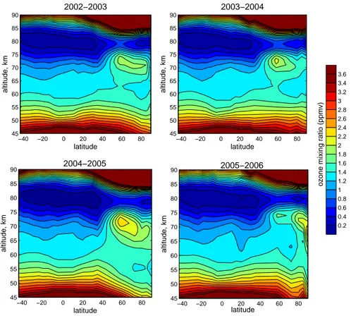
Figure 3 shows altitude-latitude dependence of GOMOS zonal mean ozone mixing ratios averaged over the period 15 December–15 January, for four NH winters The latitudinal grid used in Fig. 3 is not uniform; it is spaced according to data availability

10

(see Fig. 1). At high latitudes, the width of latitudinal bins is 5◦. The peak mixing ratio is located at altitudes 65–75 km, and usually its latitudinal position is close to the po-lar night terminator. Unlike the modelling results by Hartogh et al. (2004), the tertiary ozone maximum is not clearly isolated from the high latitudes as predicted by Fig. 9 in (Hartogh et al., 2004). In addition, (Hartogh et al., 2004) predicts large ozone values

15

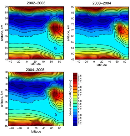
around the pole at upper altitudes (down to 75 km) indicating strong downward trans-port of atomic oxygen from the thermosphere, which is not confirmed by the GOMOS data.

Figure 4 shows the analogous latitude-altitude sections obtained from WACCM simu-lations. The midnight model data for 0◦were averaged over three ensemble simulations

20

and over the same time period 15 December–15 January, as the GOMOS data. The distributions look similar, but the model ozone mixing ratios are∼50% higher than in the GOMOS data. This disagreement is unlikely explained by the remaining differences in data averaging (GOMOS zonal mean versus WACCM data for 0◦longitude averaged over the three ensemble realizations): from GOMOS measurement, we selected data

25

(8)

ACPD

9, 6597–6615, 2009

maximum

Title Page

Tables Figures

◭ ◮

Back Close

Full Screen / Esc

Interactive Discussion According to Figs. 3 and 4, the tertiary ozone maximum can extend to the pole. This

extension varies from year to year. It seems that the appearance of tertiary ozone max-imum close to the pole is related to the intensity of horizontal mixing at high latitudes (see also below).

It is interesting that the altitude position of the tertiary ozone maximum shifts

down-5

ward with moving closer to the pole. This might be related to the downward transport in the polar night area and can illustrate the peculiarities of the meridional circulation.

5 Dynamical aspects

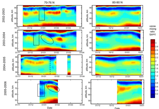
In order to follow the evolution of tertiary ozone during polar night, we selected two lat-itudinal bands in NH: 70◦–76◦N and 80◦–90◦N. These latitudinal bands have a very

10

good daily coverage by occultations of the brightest stars (Sirius, Rigel, Procyon), which allow very accurate ozone measurements.

The time series of ozone mixing ratio in the mesosphere in two latitudinal bands, for four Northern Hemisphere winters are shown in Fig. 5. Based on the modelling results by Hartogh et al. (2004, Figs. 5 and 6), one would expect that the seasonal variations

15

of tertiary ozone maximum at these latitudes consist of two isolated peaks in the be-ginning (October–November) and at the end (February–March) of winter, according to the variation of the polar night terminator. However, the seasonal variations of ozone mixing ratio in Fig. 5 do not show such behavior. As seen in Fig. 5, the tertiary ozone maximum is observed usually throughout the winter, but its magnitude is subject to

20

significant variations.

During sudden stratospheric warmings, the tertiary ozone mixing ratio can decrease significantly, as during the major stratospheric warming in December 2003 (Manney et al., 2005), or even the tertiary ozone maximum can be completely destroyed, as during the stratospheric warming in late January 2006, as seen in Fig. 5. Due to a

25

(9)

ACPD

9, 6597–6615, 2009

maximum

Title Page

Tables Figures

◭ ◮

Back Close

Full Screen / Esc

Interactive Discussion particular, two very strong downward transport events – in January 2004 discussed in

(Hauchecorne et al., 2007) and in February–March 2006 discussed in (Randall et al., 2006) – are clearly observed in Fig. 5. It is interesting that strong downward transport is observed after sudden stratospheric warmings.

Comparing Fig. 5 and Fig. 3, one might suggest that there exists a relationship

5

between the isolation of the tertiary ozone maximum from the pole and intensity of downward transport. Since the data shown in Fig. 3 are averaged over the period 15 December–15 January, only one subplot in Fig. 3, for winter 2003–2004, includes the period of strong downward transport. The tertiary ozone maximum is more iso-lated from the pole for 2003–2004 than for other years. It seems that cases with strong

10

downward transport also have a decrease in horizontal mixing, thus resulting in a better isolation of tertiary ozone maximum from the pole, and vice versa.

6 Influence of energetic particles precipitation

Energetic particle precipitation events, such as Solar Proton Events (SPE), produce HOxin the high latitude middle atmosphere, including the polar night terminator region

15

where the tertiary ozone maximum is formed. Increased ionization caused by particle precipitation leads to HO_x production via ion chemical reactions (e.g., Solomon et al., 1981). Theoretical predictions of significant HOxproduction and the subsequent ozone

loss have been verified by the observations of MLS/Aura and GOMOS/Envisat instru-ments (Verronen et al., 2006). In the terminator area the HO_xconcentration is relatively

20

low, therefore moderate SPE production can compensate for the reduced natural HOx

production in the terminator area and can even exceed it. Sepp ¨al ¨a et al. (2006) have shown that the tertiary ozone maximum disappeared during the January 2005 SPE. Figure 6 presents another example/confirmation of TOM sensitivity to particle forc-ing, the destruction of TOM by the moderate SPE of December 2006. Larger values

25

∼2 ppmv are seen at 65–70 km until 7 December when the SPE began. After the onset

(10)

recov-ACPD

9, 6597–6615, 2009

maximum

Title Page

Tables Figures

◭ ◮

Back Close

Full Screen / Esc

Interactive Discussion ery on 16 December when the SPE particle forcing declines to the quiet-time level.

Because of the short photochemical lifetime of HOx, low ozone values are observed

only when the particle fluxes are elevated. As the forcing stops, the HOx production

also stops and the HO_x amount returns to normal level within a day, thus resulting in ozone recovery. SPE cause pronounced changes in TOM, because they are sporadic

5

and typically last only for several days. On the other hand, electron precipitation in the auroral oval region also affects TOM. Electron precipitation is more continuous but of lower intensity compared to SPE. For example, in Fig. 5 the largest ozone mixing ratios are observed in January–February 2006 when energetic particle forcing was lowest in 2002–2006 as indicated by geomagnetic activity indices (Sepp ¨al ¨a et al., 2007). This

10

indicates the importance of including particle precipitation in models in order to obtain quantitative agreement with measurements in the mesosphere.

7 Summary

In this paper, we show the first experimental global distribution and seasonal variations of the tertiary ozone maximum in 2002–2006, as obtained from GOMOS data. The

15

tertiary ozone maximum is observed at high latitudes in winter. Peak ozone mixing ratio is from 2 to 4 ppm, and it can be observed at altitudes 65–75 km, depending on latitude and time. The obtained distributions can be used for validation of global circulation and chemical transport models.

The WACCM model predicts well the position of tertiary ozone maximum and its

20

latitudinal extent, thus confirming general understanding of the processes related to the formation of tertiary ozone maximum. Peak concentrations are slightly overestimated in WACCM compared to GOMOS data.

Energetic particle precipitation significantly affects the ozone concentrations at the location of the tertiary maximum (and in the mesosphere in general). Even moderate

25

(11)

ACPD

9, 6597–6615, 2009

maximum

Title Page

Tables Figures

◭ ◮

Back Close

Full Screen / Esc

Interactive Discussion in the Northern Hemisphere in January–February 2006. This indicates the importance

of including energetic particle precipitation in models of the middle atmosphere.

Acknowledgements. The work of VS, PV and AS was supported by the Academy of Finland (postdoctoral research projects of VS and AS, THERMES project). The National Center for Atmospheric Research is operated by the University Corporation for Atmospheric Research 5

under sponsorship of the National Science Foundation.

References

Bertaux, J. L., Hauchecorne, A., Dalaudier, F., Cot, C., Kyrola, E., Fussen, D., Tammi-nen, J., Leppelmeier, G. W., Sofieva, V., HassiTammi-nen, S., Fanton d’Andon, O., Barrot, G., Mangin, A., Theodore, B. Guirlet, M. Korablev, O., Snoeij, P. Koopman, R., and Fraisse, 10

R.: First results on GOMOS/Envisat, Advances in Space Research, 33, 1029–1035, doi:10.1016/j.asr.2003.09.037, 2004.

Collins, W. D., Rasch, P. J., Boville, B. A., Hack, J. J., McCaa, J. R., Williamson, D. L., Kiehl, J. T., and Briegleb, B.: Description of the NCAR Community Atmosphere Model (CAM 3.0), Natl. Cent. for Atmos. Res., Boulder, Colorado, USA, 2004.

15

Garcia, R. R., Marsh, D. R., Kinnison, D. E., Boville, B. A., and Sassi, F.: Simulation of secular trends in the middle atmosphere, 1950–2003, J. Geophys. Res., 112, D09301, doi:10.1029/2006JD007485, 2007.

Grenfell J. L., Lehmann, R., Mieth, P., Langematz, U., and Steil, B.: Chemical reaction pathways affecting stratospheric and mesospheric ozone, J. Geophys. Res., 111, D17311, 20

doi:10.1029/2004JD005713, 2006.

Hartogh, P., Jarchow, C., Sonnemann, G. R., and Grygalashvyly, M.: On the spatiotemporal behavior of ozone within the upper mesosphere/mesopause region under nearly polar night conditions, J. Geophys. Res., 109, D18303, doi:10.1029/2004JD004576, 2004.

Hauchecorne, A., Bertaux, J.-L., Dalaudier, F., Russell III, J. M., Mlynczak, M. G., Kyr ¨ol ¨a, E., 25

and Fussen, D.: Large increase of NO₂in the north polar mesosphere in January–February 2004: Evidence of a dynamical origin from GOMOS/ENVISAT and SABER/TIMED data, Geophys. Res. Lett., 34, L03810, doi:10.1029/2006GL027628, 2007.

Hedin, A. E.: Extension of the MSIS Thermosphere Model into the Middle and Lower Atmo-sphere, J. Geophys. Res., 96(A2), 1159–1172, 1991.

(12)

ACPD

9, 6597–6615, 2009

maximum

Title Page

Tables Figures

◭ ◮

Back Close

Full Screen / Esc

Kyr ¨ol ¨a, E., Sihvola, E., Kotivuori, Y., Tikka, M., Tuomi, T., and Haario, H.: Inverse theory for occultation measurements: 1. Spectral inversion, J. Geophys. Res., 98(D4), 7367–7381, 1993.

Kyr ¨ol ¨a, E., Tamminen, J., Leppelmeier, G. W., Sofieva, V., Hassinen, S., Bertaux, J. L., Hauchecorne, A., Dalaudier, F., Cot, C., Korablev, O., Fanton d’Andon, O., Barrot, G., Man-5

gin, A., Theodore, B., Guirlet, M., Etanchaud, F., Snoeij, P., Koopman, R., Saavedra, L., Fraisse, R., Fussen, D., and Vanhellemont, F.: GOMOS on Envisat: An overview, Advances in Space Research, 33, 1020–1028, doi:10.1016/S0273-1177(03)00590-8, 2004.

Kyr öl ä, E., Tamminen, J., Leppelmeier, G. W., Sofieva, V., Hassinen, S., Sepp äl ä, A., Verronen, P. T., Bertaux, J. L., Hauchecorne, A., Dalaudier, F., Fussen, D., Vanhellemont, F., Fanton 10

d’Andon, O., Barrot, G., Mangin, A., Theodore, B., Guirlet, M., Koopman, R., Saavedra de Miguel, L., Snoeij, P., Fehr, T., Meijer, Y., and Fraisse, R.: Nighttime ozone profiles in the stratosphere and mesosphere by the Global Ozone Monitoring by Occultation of Stars on Envisat, J. Geophys. Res., 111, D24306, doi:10.1029/2006JD007193, 2006.

Lin, S.-J.: A vertically Lagrangian finite-volume dynamical core for global models, Mon. Weather 15

Rev., 132, 2293–2307, 2004.

Manney, G. L., Kr ¨uger, K., Sabutis, J. L., Sena, S. A., and Pawson, S.: The remarkable 2003– 2004 winter and other recent warm winters in the Arctic stratosphere since the late 1990s, J. Geophys. Res., 110, D04107, doi:10.1029/2004JD005367, 2005.

Marsh, D., Smith, A., Brasseur, G., Kaufmann, M., and Grossmann, K.: The existence of 20

a tertiary ozone maximum in the high-latitude middle mesosphere, Geophys. Res. Lett., 28(24), 4531–4534, 2001.

Marsh, D. R., Garcia, R. R., Kinnison, D. E., Boville, B. A., Sassi, F., Solomon, S. C., and Matthes, K.: Modeling the whole atmosphere response to solar cycle changes in radia-tive and geomagnetic forcing, J. Geophys. Res., 112, D23306, doi:10.1029/2006JD008306, 25

2007.

Randall, C. E., Harvey, V. L., Singleton, C. S., Bernath, P. F., Boone ,C. D., and Kozyra, J. U.: Enhanced NO_x in 2006 linked to upper stratospheric Arctic vortex, Geophys. Res. Lett., 33, L18811, doi:10.1029/2006GL027160, 2006.

Sepp ¨al ¨a, A., Verronen, P. T., Sofieva, V. F., Tamminen, J., Kyrola, E., Rodger, C. J., and Clilverd, 30

M. A.: Destruction of the Tertiary Ozone Maximum During a Solar Proton Event, Geophys. Res. Lett., 33, L07804, doi:10.1029/2005GL025571, 2006.

(13)

ACPD

9, 6597–6615, 2009

maximum

Title Page

Tables Figures

◭ ◮

Back Close

Full Screen / Esc

L., and Kyr öl ä, E.: Arctic and Antarctic polar winter NOx and energetic particle precipitation in 2002–2006, Geophys.l Res. Lett., 34, L12810, doi:10.1029/2007GL029733, 2007. Sofieva, V. F., Tamminen, J., Haario, H., Kyr öl ä, E., and Lehtinen, M.: Ozone profile smoothness

as a priori information in the inversion of limb measurements, Ann. Geophys., 22, 3411– 3420, 2004a,

5

http://www.ann-geophys.net/22/3411/2004/.

Sofieva, V. F., Verronen, P. T., Kyr ¨ol ¨a, E., Hassinen, S., and GOMOS CAL/VAL team: The tertiary ozone maximum in the middle mesosphere as seen by GOMOS on Envisat, Qua-drennial Ozone Symposium, 2004b.

Solomon, S., Rusch, D. W., G ´erard, J.-C., Reid, G. C., and Crutzen, P. J.: The effect of particle 10

precipitation events on the neutral and ion chemistry of the middle atmosphere: II. Odd hydrogen, Planet. Space Sci., 8, 885–893, 1981.

Tamminen, J., Kyr ¨ol ¨a, E., and Sofieva, V.: Does a priori information improve occultation mea-surements?, in: Occultations for Probing Atmosphere and Climate, edited by: Kirchengast, G., Foelshe, U., and Steiner, A., Springer Verlag, 87–98, 2004.

15

(14)

ACPD

9, 6597–6615, 2009

maximum

Title Page

Tables Figures

◭ ◮

Back Close

Full Screen / Esc

Interactive Discussion ≥

Fig. 1. Location of GOMOS nighttime occultations of starts with the e_ffective temperature

(15)

ACPD

9, 6597–6615, 2009

maximum

Title Page

Tables Figures

◭ ◮

Back Close

Full Screen / Esc

Jan03 Jan04 Jan05 Jan06

−80 −60 −40 −20 0 20 40 60 80

date

latitude

Jan03 Jan04 Jan05 Jan06

−80 −60 −40 −20 0 20 40 60 80

date

latitude

0.5 1 1.5 2 2.5 3

GOMOS

WACCM

ozone mixing ratio (ppmv)

Fig. 2.Ozone mixing ratio at 72 km. Top: from GOMOS measurements (zonal mean), bottom:

(16)

ACPD

9, 6597–6615, 2009

maximum

Title Page Abstract Introduction Conclusions References Tables Figures ◭ ◮ ◭ ◮ Back Close

Full Screen / Esc

Interactive Discussion latitude

altitude, km

2002−2003

−40 −20 0 20 40 60 80

45 50 55 60 65 70 75 80 85 90 latitude altitude, km 2003−2004

−40 −20 0 20 40 60 80

ozone mixing ratio (ppmv)

−40 −20 0 20 40 60 80

45 50 55 60 65 70 75 80 85 90 0.2 0.4 0.6 0.8 1 1.2 1.4 1.6 1.8 2 2.2 2.4 2.6 2.8 3 3.2 3.4 3.6

Fig. 3. Latitude-altitude section of GOMOS zonal mean ozone mixing ratio distribution (ppmv)

(17)

ACPD

9, 6597–6615, 2009

maximum

Title Page

Tables Figures

◭ ◮

Back Close

Full Screen / Esc

Interactive Discussion latitude

altitude, km

2002−2003

−40 −20 0 20 40 60 80

45 50 55 60 65 70 75 80 85 90

latitude

altitude, km

2003−2004

−40 −20 0 20 40 60 80

45 50 55 60 65 70 75 80 85 90

latitude

altitude, km

2004−2005

ozone mixing ratio (ppmv)

−40 −20 0 20 40 60 80

45 50 55 60 65 70 75 80 85 90

0.2 0.4 0.6 0.8 1 1.2 1.4 1.6 1.8 2 2.2 2.4 2.6 2.8 3 3.2 3.4 3.6

Fig. 4.Altitude-latitude sections from WACCM simulations. The data for midnight at longitude

(18)

ACPD

9, 6597–6615, 2009

maximum

Title Page Abstract Introduction Conclusions References Tables Figures ◭ ◮ ◭ ◮ Back Close

Full Screen / Esc

Printer-friendly Version Interactive Discussion a lti tu d e , k m 70-76 N 2002-2003

01/11 01/12 01/01 01/02 01/03 01/04

50 60 70 80 a lti tu d e , k m 2003-2004

01/11 01/12 01/01 01/02 01/03 01/04

50 60 70 80 a lti tu d e , k m 2004-2005

01/11 01/12 01/01 01/02 01/03 01/04

50 60 70 80 Date al ti tude , k m 2005-2006

01/11 01/12 01/01 01/02 01/03 01/04

50 60 70 80 a lti tu d e , k m 80-90 N

01/12 15/12 01/01 15/01

50 60 70 80 a lti tu d e , k m 15/12

01/12 01/01 15/01

50 60 70 80 a lti tu d e , k m 15/12

01/12 01/01 15/01

50 60 70 80 Date a lti tu d e , k m

01/12 15/12 01/01 15/01

50 60 70 80 0.2 0.4 0.6 0.8 1 1.2 1.4 1.6 1.8 2 2.2 2.4 2.6 2.8 3 ozone mixing ratio (ppm)

Fig. 5. Time series of zonal mean ozone mixing ratio profiles are shown for two latitudinal

(19)

ACPD

9, 6597–6615, 2009

maximum

Title Page

Tables Figures

◭ ◮

Back Close

Full Screen / Esc

altitude, km

Ozone mixing ratio

Day in December 2006

04 05 06 07 08 09 10 11 12 13 14 15 16 17 18 19 20 21 22 23 24 25 26 27 28 29 30 45

50 55 60 65 70 75 80 85

04 05 06 07 08 09 10 11 12 13 14 15 16 17 18 19 20 21 22 23 24 25 26 27 28 29 30 100

102 104

Day in December 2006

proton flux [protons cm

−2

s−1 sr

−1

] GOES−11 integral proton flux

> 5 MeV > 10 MeV > 30 MeV

0.5 1 1.5 2 2.5

Fig. 6. Top: daily ozone mixing ratio profiles at latitudes 60–90 N in December 2006. Bottom: