Technical note: Functional sliced inverse regression to infer temperature, water vapour and ozone from IASI data

(1)

ACPD

9, 7589–7613, 2009

Dimension-reduction for IASI radiances

U. Amato et al.

Title Page

Abstract Introduction

Conclusions References

Tables Figures

◭ ◮

Back Close

Full Screen / Esc

Printer-friendly Version

Interactive Discussion

Atmos. Chem. Phys. Discuss., 9, 7589–7613, 2009 www.atmos-chem-phys-discuss.net/9/7589/2009/ © Author(s) 2009. This work is distributed under the Creative Commons Attribution 3.0 License.

Atmospheric Chemistry and Physics Discussions

This discussion paper is/has been under review for the journalAtmospheric Chemistry

and Physics (ACP). Please refer to the corresponding final paper inACPif available.

Technical note: Functional sliced inverse

regression to infer temperature, water

vapour and ozone from IASI data

U. Amato1, A. Antoniadis2, I. De Feis1, G. Masiello3, M. Matricardi4, and C. Serio3

1

Istituto per le Applicazioni del Calcolo “Mauro Picone” CNR, Napoli, Italy

2

Laboratoire Jean Kuntzmann, Universit ´e Joseph Fourier, Grenoble, France

3

Dipartimento di Ingegneria e Fisica dell’Ambiente, Universit `a della Basilicata, Potenza, Italy

4

European Centre for Medium-Range Weather Forecasts (ECMWF), Reading, UK

Received: 7 January 2009 – Accepted: 10 March 2009 – Published: 23 March 2009

Correspondence to: I. De Feis (i.defeis@iac.cnr.it)

(2)

ACPD

9, 7589–7613, 2009

U. Amato et al.

Title Page

Tables Figures

◭ ◮

Back Close

Full Screen / Esc

Interactive Discussion Abstract

A retrieval algorithm that uses a statistical strategy based on dimension reduction is proposed. The methodology and details of the implementation of the new algorithm are presented and discussed. The algorithm has been applied to high resolution spectra measured by the Infrared Atmospheric Sounding Interferometer instrument to retrieve

5

atmospheric profiles of temperature, water vapour and ozone. The performance of the inversion strategy has been assessed by comparing the retrieved profiles to the ones obtained by co-locating in space and time profiles from the European Centre for Medium-Range Weather Forecasts analysis.

1 Introduction

10

The development of satellite high-spectral resolution infrared spectrometers is ex-pected to improve quality and density of retrieval of atmospheric parameters. Both Nu-merical Weather Prediction and Earth’s monitoring are expected to benefit from these new modern sensors.

The pioneer of this new generation of instruments has been the Interferometric

Mon-15

itor for Greenhouse (IMG) gases sensor (Kobayashi et al., 1999), that flew on the AD-vanced Earth Observing Satellite (ADEOS) platform from August 1996 to June 1997. At present, high-resolution infrared sensors on operational meteorological polar or-biters include the Atmospheric Infrared Sounder (AIRS) on the second Earth Observ-ing System (EOS) polar orbitObserv-ing platform, EOS-Aqua, launched in April 2002 (Aumann

20

and Pagano, 1994), and the Tropospheric Emission Spectrometer (TES) on the AURA satellite launched in 2004 (Beer et al., 2001).

The new arrived in the family of high resolution infrared sensors is the Infrared At-mospheric Sounding Interferometer (IASI) (EUMETSAT, 1998) on the first European Meteorological Operational Satellite (METOP/1) launched in 19 October 2006. IASI

25

is a Fourier Transform Spectrometer based on a Michelson Interferometer coupled to

(3)

ACPD

9, 7589–7613, 2009

U. Amato et al.

Title Page

Tables Figures

◭ ◮

Back Close

Full Screen / Esc

an integrated imaging system that observes and measures infrared radiation emitted

from the Earth in the spectral range 3.62–15.5 µm (645–2760 cm−1), covering the peak

of the thermal infrared and particularly the intense CO2 band around 666 cm−1, with

an apodized resolution of 0.5 cm−1 and a spectral sampling of 0.25 cm−1. IASI

char-acteristics have been specified to get observations, which are compatible in terms of

5

sampling, resolution, accuracy and overall performances with the mission objectives of providing improved information on temperature, water vapour, ozone, cloud top pres-sure and temperature, cloud cover and cloud optical properties.

The large amount of observed data needs algorithms for the radiative transfer equa-tion and its inversion specifically designed for IASI. In this paper we describe a

statisti-10

cal regression methodology for temperature, water vapour and ozone, (T, q, o), which

exploits IASI observations. The methodology is based on a suitable statistical dimen-sion reduction technique, FSIR (Functional Sliced Inverse Regresdimen-sions. FSIR (Amato

et al., 2006) generalizes the well known Principal Component Analysis (PCA) (Jolliffe,

2002, e.g.) or Empirical Orthogonal Function (EOF) approach (see the recent review

15

on EOF regression methods by Serio et al., 2008a) and allows one to deal with func-tional models.

FSIR needs to be trained on a suitable set of pairs: radiances, profiles. We have selected the profiles from the well known ECMWF (European Centre for Medium-range Weather Forecasts) Chevalier data base (Chevalier, 2001); IASI synthetic radiances

20

have been computed using the radiative transfer codeσ-IASI (Amato et al., 2002).

The code σ-IASI has been extensively validated with the use of the NAST-I

instru-ment (Cousins and Gazarick, 1999, e.g.). NAST-I is the NPOESS Airborne Sounder Testbed Fourier Transform spectrometer, flying onboard the NASA aircrafts, ER-2

and Proteus. An extensive retrieval exercise withσ-IASI has been performed for the

25

CAMEX/3 experiment (Convection and Moisture Experiment 3) (Carissimo et al., 2005,

2006, e.g.). More recently,σ-IASI has also been used within the EAQUATE campaign

(4)

ACPD

9, 7589–7613, 2009

U. Amato et al.

Title Page

Tables Figures

◭ ◮

Back Close

Full Screen / Esc

2007). The forward moduleσ-IASI has been also validated with the use of AIRS

(At-mospheric Infrared Radiometer Sounder) data, flying onboard the Aqua satellite (Saun-ders et al., 2007).

The application of FSIR to IASI data has been exemplified through a series of IASI

soundings recorded over the tropical basin. These observation have been

FSIR-5

regressed for (T, q, o). To simplify the comparison of retrieval products withtruthdata,

only clear-sky, sea-surface IASI soundings have been analyzed in this work. Truth data have been derived from the ECMWF analysis for the same date and location as the

IASI soundings. The difference (retrieval-ECMWF) for temperature, water vapour and

ozone has been evaluated, which has allowed us to assess the retrieval performance

10

of FSIR. The paper also provides a comparison with a conventional EOF or PCA re-gression scheme (see also Serio et al., 2008a).

The paper is organized as follows. Section 2 will deal with the mathematical aspects of FSIR. Application of FSIR to IASI data will be described and discussed in Sect. 4. Finally conclusions will be drawn in Sect. 5.

15

2 The regression model

Functional Sliced Inverse Regression (FSIR) (Amato et al., 2006) is a statistical tool to reduce the dimensionality based on the Sliced Inverse Regression (SIR) (Li, 1991), that permits to deal with functional models. It generalizes the Principal Component Analysis (PCA) using inverse regression.

20

In functional regression problems, one predicts a response variableY from a set of

variablesR1, . . . , Rd that are discretizations of a same curveRat pointsν1, . . . , νd, that

isR_j=R(ν_j), j=1, . . . , d, where the discretization pointsν_j lie in some interval. In our

caseY is the geophysical variable to be retrieved (surface temperature, temperature

or gas concentration in a fixed layer) and R1, . . . , Rd are the measurements, i.e., the

25

radiances at wavenumbersν1, . . . , νd. Let us consider the model

Y =m hβ1,Ri, . . . ,hβK,Ri

+ε , (1)

(5)

ACPD

9, 7589–7613, 2009

U. Amato et al.

Title Page

Tables Figures

◭ ◮

Back Close

Full Screen / Esc

where m is a smooth link function of the K-dimensional Euclidean space, EK, into

the one-dimensional space or real axisE1, εis noise assumed independent of R(ν),

{βi(ν), i=1, . . . , K} are K orthonormal functions. The symbol h·,·i denotes the usual

inner product.

Let ΣR be the covariance operator of R(ν) and Σe the covariance operator of the

5

conditional expected value,E(R|Y), of the radiance given the geophysical variable to

retrieve.

Provided thatK <d, the regression function depends onR(ν) only through K linear

functionals of the explanatory processR(ν). Hence, to explain the dependent variable

Y, the space of d explanatory variables can be reduced to a space with a smaller

10

dimension K. The dimension reduction methods aim at finding the dimension K of

the reduction space and a basis defining this space. The functionsβi,i=1, . . . , K, are

called effective dimension reduction (edr)-directions and the space they generate is the

edr-space.

FSIR is able to work with this model, indeed it yieldsd directions ˆβi and

correspond-15

ing (eigen-)values ˆλ_i which allow one to rank the importance of ˆβ_i. The technique

takes advantage of the method of inverse regression. Here the aim is not to estimate

E[Y|R₌r] but the reverseE[R|Y=y], a one-dimensional regression problem that avoids

the curse of dimensionality. This curse means that high-dimensional spaces have too

few data for local averaging. Instead of having one d-dimensional regression

prob-20

lem we have d one-dimensional regression problems which do not su_ffer from that

curse. The key of FSIR is the connection between the edr-space and the inverse

re-gression curve given by the covariance operator of the inverse rere-gression curve Σe.

Indeed it is possible to prove under some mild assumptions (Amato et al., 2006) that

the eigenvalue-eigenvector decomposition of the operator Σ−1_R Σe permits to identify

25

a basis for the edr-space. Unfortunately the inverse ofΣRis not bounded, therefore we

considerΣ−1_R /2ΣeΣ

−1/2

R ; in particular, we use the fact thatΣ

−1/2

R ΣeΣ

−1/2

R has the same

eigenvectors asΣ1_R/2Σ+eΣ

1/2

R , whereΣ

+

(6)

op-ACPD

9, 7589–7613, 2009

U. Amato et al.

Title Page

Tables Figures

◭ ◮

Back Close

Full Screen / Esc

erator (Groetsch, 1974).

Let us now consider a dataset ofN radiance spectra measured at wavenumbersνj,

j=1, . . . , d, and corresponding profiles Y_N, that is (R_n, Y_n),n=1, . . . , N, withR_n being

vectors of dimensiond×1. Then after centering the data,ΣRcan be estimated by

ˆ

ΣR,N =

1

N

N X

n=1

RnRtn. (2)

5

For the estimate ofΣewe may proceed in the following way. LetMY(ν)=E(R|Y) and

ˆ

MY(ν) be the wavelet smoothing of R(ν) with design points the Yn’s, n=1, . . . , N,

ob-tained through the BINWAV estimator (Antoniadis and Pham, 1998). Then we consider the following estimate forΣe:

ˆ

Σe,N =

1

N

N X

n=1

ˆ

MY_nMˆ

t

Y_n, (3)

10

with Mˆ_Y_n=( ˆMYn(νj))j=1...,d=(E(Rj|Y=Yn))j=1...,d a vector of dimension d×1 for each

n=1, . . . , N.

Convergence in probability of bothΣˆR,N andΣˆe,N toΣRandΣecan be found in

(Am-ato et al., 2006). To estimate them accurately, we improve the conditioning of Σˆe,N

applying a projector method before performing the spectral decomposition: let ˆπ_k_N

de-15

note the orthogonal projector into the space spanned by thekN eigenvectors of Σˆe,N

corresponding to thekN largest eigenvalues; we letΣˆ

k_N

e,N=πˆkNΣˆe,N πˆkN. Estimation of

the EDR space is derived from the spectral decomposition of

ˆ

Σ1_R,N/2 Σˆ_e,NkN +Σˆ1_R,N/2 , (4)

where Σˆk_e,NN + is the pseudoinverse matrix defined through the Singular Value

De-20

composition (SVD) (Golub and Van Loan, 1983; Golub, 1970). Let (α_i)_i₌1,...,K be the

(7)

ACPD

9, 7589–7613, 2009

U. Amato et al.

Title Page

Tables Figures

◭ ◮

Back Close

Full Screen / Esc

smallest eigenvalues of (4) andη_i the corresponding eigenfunctions, then

ˆ

βN_i = 1

αi

ˆ

Σk_e,NN +Σˆ1_R,N/2η_i. (5)

Summarizing the procedure for computing an estimate ˆβNi =( ˆβi(ν1), . . . ,βˆi(νd))t of the

EDR directionsβ_i,i=1, . . . , K, goes through the following steps:

Algorithm

5

1. calculate ˆMY(ν), the wavelet smoothing ofR(ν) with design pointsY1, . . . , YN,

us-ing the BINWAV estimator and evaluate it inν1, . . . , νd;

2. estimate ˆΣR,N by Eq. (2) and ˆΣe,N by Eq. (3);

3. evaluate the spectral decomposition of ˆΣe,N and its projection ˆΣ

kN

e,N;

4. evaluate the spectral decomposition of ˆΣ1_R,N/2 Σˆ_e,NkN +Σˆ1_R,N/2 and estimate the EDR

10

directions by Eq. (5).

FSIR can be seen as a generalization of PCA. Indeed supposing thatΣRis the

iden-tity operator, than FSIR aims at determining the directions along which to project the

data by the eigenvalues-eigenvectors decomposition of Σe, which takes into account

the information about the profiles by means of a regression on the spectra; on the

15

contrary the PCA uses only spectral information.

3 Vertical resolution of the retrieval

(8)

ACPD

9, 7589–7613, 2009

U. Amato et al.

Title Page

Tables Figures

◭ ◮

Back Close

Full Screen / Esc

the retrieval covariance matrix can be obtained by

Σ_Yˆ =E

( ˆY −Ytrue)( ˆY −Ytrue)t

, (6)

where expectation value has to be taken with respect to training data set andY_trueis

thetrue value of the parameter. This matrix will be denoted by ΣT,ΣH2O and ΣO3 for

temperature, water vapour and ozone profiles, respectively.

5

The retrieval covariance matrix, for a given parameter profile, can be used to analyze the spatial vertical resolution of the parameter itself, according to a methodology which has been developed by Serio et al. (2008b) and which is summarized for the sake of clarity.

The vector (Y(1), Y(2), . . . , Y(M))t represents the discretized version of a spatial

10

function (i.e., temperature profile, water vapour mixing ratio profile, ozone mixing ratio profile). A strong correlation, that is a relatively high value of the covariance, between any two of the parameters means that the two have not been independently resolved by the data set, and that only some linear combination of the parameters is resolved.

However, a direct examination and interpretation of the off-diagonal elements

(covari-15

ances) of a covariance operator is not easy, which makes the definition of some suitable scalar index high desirable.

To this end, it has to be considered that the retrieval correlation is determined by

the non-null off-diagonal terms in the covariance operator. For a full independent

re-trieval (and therefore for a rere-trieval, which attains the maximum possible vertical spatial

20

resolution), the covariance matrix has to be fully diagonal.

In what follows we will assume that the covariance operator has been normalized in order to obtain the correlation matrix,

Σ_Yˆ(i , j)←

Σ_Yˆ(i , j)

p

Σ_Yˆ(i , i)Σ_Yˆ(j, j)

. (7)

Σ_Yˆ may be additively decomposed in its diagonal and off-diagonal components:

25

Σ_Yˆ =Σ_Yˆ_,_diag+Σ_Yˆ_,_o_ff. (8)

(9)

ACPD

9, 7589–7613, 2009

U. Amato et al.

Title Page

Tables Figures

◭ ◮

Back Close

Full Screen / Esc

An index which assesses the dominance of the diagonal term over the off-diagonal

one might be simply defined from the norms of the matrices in Eq. (8). However, the norm is not additive. In general, we have

norm(Σ_Yˆ)6=norm(Σ_Yˆ_,_diag)+norm(Σ_Yˆ_,_o_ff) ; (9)

therefore, an index such as the ratio of theΣ_Yˆ, diag-norm to theΣ_Yˆ-norm is not well

5

defined. It could be less or greater than one depending on the given matrix.

To quantify the relative contribution of the diagonal term (and off-diagonal term) to

the norm ofΣ_Yˆ, let us consider the SVD ofΣ_Yˆ. With the usual notation, we have

ΣYˆ =ΣYˆ,diag+ΣYˆ,off =USYˆVt (10)

where U and V are unit, orthogonal matrices of size M by M; S is a diagonal

ma-10

trix whose elements are the eigenvalues, positive definite and supposed decreasingly

ordered, of the operatorΣYˆ. From the equation above, we have

UtΣ_Yˆ_,_diagV+UtΣ_Yˆ_,_o_ffV=S_Yˆ (11)

which with the position

B_Yˆ_,_diag=UtΣ_Yˆ_,_diagV

B_Yˆ_,_o_ff = UtΣ_Yˆ_,_o_ffV

(12)

15

gives

B_Yˆ_,_diag+B_Yˆ_,_o_ff =SYˆ (13)

Finally, because of the definition of norm (e.g. Golub and Van Loan, 1983), we have

norm(ΣYˆ)=SYˆ(1,1)=BYˆ,diag(1,1)+BYˆ,off(1,1), (14)

whereX(1,1) is the element (1,1) of the given matrix X. The formula above is fully

20

(10)

ACPD

9, 7589–7613, 2009

U. Amato et al.

Title Page

Tables Figures

◭ ◮

Back Close

Full Screen / Esc

diagonal and off-diagonal contribution. Thus, a proper index which quantifies the

de-gree of diagonalization ofΣYˆ, that is how much the matrix is dominated by its diagonal

terms, can be defined by

i_D= BYˆ,diag(1,1)

S_Yˆ(1,1)

. (15)

For a full diagonal matrix, we havei_D=1 and the retrieval is truly independent, whereas

5

for a highly correlated matrix, we haveiD=M−1. The index (15) can be easily re-scaled

to the range 1 toM by simply redefining it as

i_D=MBYˆ,diag(1,1)

S_Yˆ(1,1)

(16)

Then,i_D=1 simply means that for the retrieval at hand it is as if the full atmosphere had

been divided just in one layer, that is only the columnar amount of the parameter has

10

been resolved. On the opposite edge of theiD scale, we haveiD=M, and the retrieval

has been fully resolved on the grid mesh used to divide the atmosphere. Nearby layers can then, e.g., be used to form average quantities and, therefore, reduce the estimation error.

4 Application to IASI data

15

The retrieval accuracy of FSIR procedure has been assessed both on the Chevalier dataset and directly on IASI data. Analysis has focused on clear sky, sea-surface,

tropical soundings. To limit the burden of the computational effort, only nadir view

soundings have been considered.

4.1 Chevalier dataset

20

The training dataset consists of 377 (T,q,o) tropical profiles for clear-sky and sea

(11)

ACPD

9, 7589–7613, 2009

U. Amato et al.

Title Page

Tables Figures

◭ ◮

Back Close

Full Screen / Esc

These profiles are the input to theσ-IASI code (Amato et al., 2002), which has been

used to calculate the related synthetic IASI spectra at nadir view angle.

The spectral ranges used to train the regression algorithm include the intense

CO₂ band 645 cm−1–830 cm−1, the ozone band 1010 cm−1–1070 cm−1, the window

1130 cm−1–1180 cm−1, a portion of theν2 water vapour band, 1400 cm

−1

–1700 cm−1,

5

and the C2O/N2O shortwave absorption band, 2000 cm

−1

–2230 cm−1, for a total of

3305 channels. Thus, the data space is made up of radiance vectors of sized=3305.

The parameter space is made up of triplets (Tj, qj, oj) for each given atmospheric

layer. The number of layers,ML, is the same as in σ-IASI, namely ML=60. For

tem-perature we have one more parameter, since we consider the surface temtem-perature, as

10

well.

The FSIR is implemented according to a single parameter regression algorithm, in

which each single element of the triplet (T_j, q_j, o_j) is regressed vs. the EDR

compo-nents.

Similarly to the EOF methodology, the FSIR approach also requires that the user

15

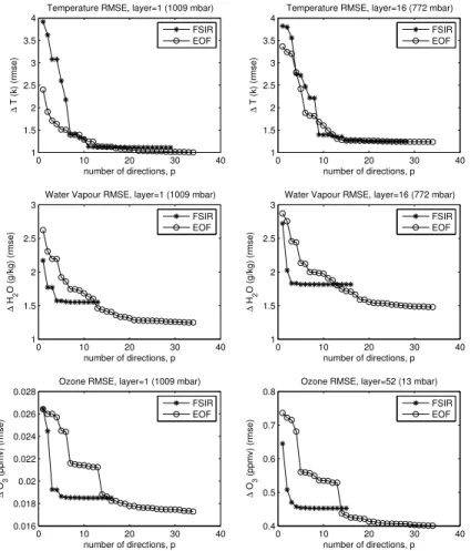
specifies the number of EDR components, p, (also called scores). To this purpose

we define the root mean square error or estimation error, e(p), of the regression as

e(p)=E[( ˆY−YChev) 2

]1/2, where, as before, E[·] means expectation value, again Y

de-notes a generic parameter andYChev refers to values from the Chevalier dataset. Our

algorithm is developed in the general context of a signal plus noise model (see, e.g.,

20

Eq. 1), therefore the curve e(p) reaches a sort of plateau or noise floor. A suitable

choice forpis the closest value to the knee of the curve,e(p) (see Serio et al., 2008a).

Examples of these curves are shown in Fig. 1, which also provides a comparison with a PCA/EOF regression approach. Based on these curves the number of scores

for whiche(p) reaches a plateau ranges betweenp=5 andp=20. Also note that FSIR

25

(12)

ACPD

9, 7589–7613, 2009

U. Amato et al.

Title Page

Tables Figures

◭ ◮

Back Close

Full Screen / Esc

almost equivalent in terms of expected root mean square error. For water vapour FSIR is superior to EOF, the same as for ozone.

4.2 iD index

Using the methodology outlined in Sect. 3, we can analyze the degree of interdepen-dency of the retrieval for temperature, water vapour and ozone. For temperature the

5

value ofiDis 6.8 for FSIR and 5.6 for EOF. This means that FSIR gains more than one

degree of freedom over the EOF regression. For water vapour and ozone we have 4.7 and 3.7, respectively, in the case of FSIR and 4.40 and 2.53 for EOF, respectively.

It is interesting to note that the FSIR retrieval is less correlated than that produced by the EOF scheme, which means that FSIR has a better capability to reveal features

10

and structures along the vertical.

However, in general the above iD values are quite small. For ozone, they indicates

that only two or three pieces of information are available for the retrieval. For

tempera-ture and water vapour,i_D says that only the very coarse features of the profile can be

resolved. This is not a serious shortcoming for temperature, which is typically a smooth

15

function of the altitude, but could become a serious limitations for water vapour, whose profile may be characterized by small-scale vertical structures.

4.3 IASI retrieval and comparison with ECMWF analysis

The FSIR approach has been tested using IASI data obtained during the IASI commis-sioning phase.

20

The cloud detection scheme described in Grieco et al. (2007) was applied to tropical spectra measured over the sea surface during the 22 July 2007. This yielded a total of 603 clear sky IASI spectra. To simplify the illustration of the results only nadir view soundings have been considered.

To develop a consistent set of truth data against which IASI retrieval could be

com-25

pared, ECMWF atmospheric analysis fields for temperature, water vapour and ozone

(13)

ACPD

9, 7589–7613, 2009

U. Amato et al.

Title Page

Tables Figures

◭ ◮

Back Close

Full Screen / Esc

were considered. These fields where co-located in space and time to the 603 IASI soundings. We used atmospheric analysis fields at 00:00, 06:00, 12:00 and 18:00 UTC on 22 July 2007. At that time, the ECMWF model was characterized by a vertical dis-cretization of the atmosphere into 60 pressure levels and a horizontal truncation of T511. This truncation corresponds to a grid spacing of about 40 km or, equivalently, to

5

a horizontal grid box of 0.351◦×0.351◦. The model has a hybrid vertical coordinate, with terrain-following coordinates in the lower troposphere and pressure coordinates in the stratosphere above about 70 hPa. Of the 60 levels in the vertical, 25 are above 100 hPa and the model top is at 0.1 hPa, corresponding to about 65 km. The vertical resolution of the analysis fields gradually decreases from 20 m at the surface to about 250 m at

10

1 km altitude, and about 1 km to 3 km in the stratosphere. The analysis fields were extracted from the ECMWF archive at the full T511 resolution, interpolated to a grid of

points with a separation of 0.3◦×0.3◦ and then co-located to the IASI soundings. The

statistics of the di_fference between global radiosonde observations and ECMWF

anal-ysis in the troposphere show values of the standard deviation typically between 0.5 K

15

and 1 K for temperature and between 0.5 and 1.5 g/kg for water vapour. In addition

to fields of temperature, water vapour and ozone, ECMWF fields of sea-surface tem-perature (SST) were also used in the study. It should be noted that these fields are based on analyses received daily from the National Centers for Environmental

Predic-tion (NCEP), Washington DC, on a 0.5◦×0.5◦grid. These analyses are based on ship,

20

buoy and satellite observations. In shallow waters, where rapid changes due to the

upwelling radiation can occur close to land, the observed SST can sometimes differ as

much as 5 K from the NCEP analysis.

One important aspect which has been possible to analyze with the help of the ECMWF analysis is the sensitivity of the retrieval accuracy to the choice of the

num-25

ber,p, of FSIR and/or PCA scores. Because of many factors, which include radiative

transfer accuracy, noise specifications, cloud contamination, in practice it may happen

that theoptimalchoice,popt, performed based on the training data set may result to be

(14)

ACPD

9, 7589–7613, 2009

U. Amato et al.

Title Page

Tables Figures

◭ ◮

Back Close

Full Screen / Esc

may occur, which is much larger than that expected on the basis of the training data set.

To address this point we have redefined the root mean square difference, e(p), as

e(p)=E[( ˆY−Yecmwf) 2

]1/2. For temperature, e(p) is shown in Fig. 3 for three values of

p, namelypopt,popt+5 andpopt+10. The calculations have been performed for FSIR

5

and PCA. It can be seen that, in comparison to EOF, FSIR is more robust in terms of

accuracy to variations in the number of scores,p. This is much more evident for the

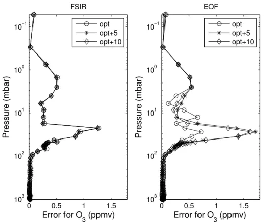
case of water vapour (Fig. 4) and ozone (Fig. 5).

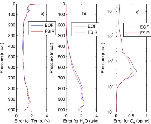
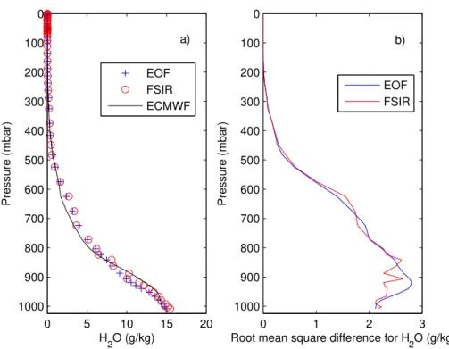
Apart from some isolated error spikes, evident in the case of ozone, FSIR also pro-vides a more accurate retrieval, once compared to EOF. This can be seen in the three

10

next Figs. 6–8 which compare FSIR performance to EOF for the case of temperature, water vapour and ozone.

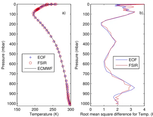
Figures 6–8 also suggest that FSIR accuracy for temperature is within 1–2 K, which is a bit larger than the 1 K expected for IASI. However, it is important to consider that the ECMWF analysis also has an uncertainty, which, as discussed above, is of the order

15

of 0.5 to 1 K. Thus ine(p) we also include the uncertainty of the ECMWF analysis.

The same as above can be said for water vapour: including the ECMWF uncer-tainty, the performance of FSIR reaches the expected accuracy of 10% only in the very deepest part of the atmosphere.

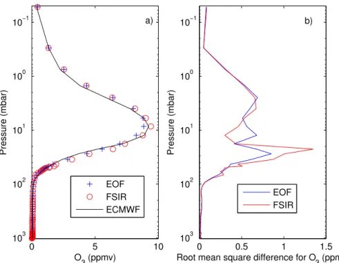
For ozone we get a very smooth retrieval, as it was expected based on theiD index

20

for this parameter. However, the result compares fairly well with ECMWF mean profile.

5 Conclusions

A new statistical strategy based on dimension reduction for then retrieval of atmo-spheric parameters from IASI radiances has been presented and discussed. Appli-cations to IASI data have been considered for the case of tropical soundings. The

25

new strategy, FSIR has been also compared to an usual EOF regression scheme. The comparison shows that, mostly for gases (we have analyzed water vapour and

(15)

ACPD

9, 7589–7613, 2009

U. Amato et al.

Title Page

Tables Figures

◭ ◮

Back Close

Full Screen / Esc

ozone), FSIR gets a higher performance with respect to EOF. In general, FSIR seems to provide a retrieval which is better resolved along the vertical, which is particularly interesting for water vapour.

For temperature the FSIR scheme provides results quite close to the expected per-formance of 1 K in the lower part of the atmosphere. For water vapour the goal of 10%

5

accuracy is reached only for the very lower part of the atmosphere.

For ozone it seems that FSIR is capable to provide at least 3 pieces of information. We think that FSIR can provide a valid initialization scheme for physical-based inver-sion strategy, issue that is now under investigation.

Acknowledgements. IASI has been developed and built under the responsibility of the Centre

10

National d’Etudes Spatiales (CNES, France). It is flown onboard the Metop satellites as part of the EUMETSAT Polar System. The IASI L1 data are received through the EUMETCast near real time data distribution service.

References

Amato, U., Antoniadis, A., and De Feis, I.: Dimension reduction in functional regression with

15

applications, Comput. Stat. Data An., 50, 2422–2446, 2006. 7591, 7592, 7593, 7594 Amato, U., Masiello, G., Serio, C., and Viggiano, M.: Theσ-IASI code for the calculation of

infrared atmospheric radiance and its derivatives, Environ. Modell. Softw., 17/7, 651–667, 2002. 7591, 7599

Antoniadis, A. and Pham, D. T.: Wavelet regression for random or irregular design, Computat.

20

Stat. Data An., 28, 353–369, 1998. 7594

Aumann, H. H. and Pagano, R. J.: Atmospheric Infrared Sounder on the Earth Observing System, Opt. Eng., 33, 776–784, 1994. 7590

Beer, R., Glavich, T. A., and Rider, D. M.: Tropospheric emission spectrometer for the earth observing system’s aura satellite, Appl. Opt., 40, 2356–2367, 2001. 7590

25

Carissimo, A., De Feis, I., and Serio, C.: The physical retrieval methodology for IASI: theσ-IASI code, Environ. Modell. Softw., 20, 1111–1126, 2005. 7591

(16)

ACPD

9, 7589–7613, 2009

U. Amato et al.

Title Page

Tables Figures

◭ ◮

Back Close

Full Screen / Esc

Interactive Discussion of the International Radiation Symposium, Busan, Korea, 23–28 August 2004, A. Deepak

Publishing, Hampton, VA, 247–250, 2006. 7591

Chevalier, F.: Sampled database of 60 levels atmospheric profiles from the ECMWF analysis, Tech. Rep., ECMWF EUMETSAT SAF programme Research Report 4, 2001. 7591, 7598 Cousins, D. and Gazarick, M. J.: NAST Interferometer Design and Characterization, Final

Re-5

port, MIT Lincoln Laboratory Project Report NOAA-26, July 13, 1999. 7591 EUMETSAT: IASI science plan, EUMETSAT, Darmstadt, 1998. 7590

Golub, G. H. and Van Loan, C. F.: Matrix Computations, Baltimore, The Johns Hopkins Univer-sity Press, 1983. 7594, 7597

Golub, G. H. and Reinsch, C.: Singular value decomposition and least squares solutions,

Nu-10

mer. Mat., 14, 403–420, 1970. 7594

Grieco, G., Masiello, G., Matricardi, M., Serio, C., Summa, D., and Cuomo, V.: Demonstration and validation of the ϕ-IASI inversion scheme with NAST-I data, Q. J. R. Meteorol. Soc., 133(S3), 217–232, 2007. 7591, 7600

Groetsch, C. W.: Generalized Inverses of Linear Operators: Representation and

Approxima-15

tion, Dekker, New York, 1977. 7594

Kobayashi, H., Shimota, A., Yoshigahara, C., Yoshida, I., Uehara, Y., and Kondo, K.: Satellite-Borne High-Resolution FTIR for Lower Atmosphere Sounding and Its Evaluation, IEEE Trans. Geosci. Remote Sens., 37, 1496–1507, 1999. 7590

Jolliffe, I. T.: Principal Component Analysis, New York, Springer-Verlag, 2002. 7591

20

Li, K. C.: Sliced inverse regression for dimension reduction, with discussions, J. Amer. Statist. Assoc., 86, 316–342, 1991. 7592

Saunders, R., Rayer, P., Brunel, P., von Engeln, A., Bormann, N., Strow, L., Hannon, S., Heilli-ette, S., Liu, X., Miskolczi, F., Han, Y., Masiello, G., Moncet, J. L., Uymin, G., Sherlock, V., and Turner, S. D.: A comparison of radiative transfer models for simulating Atmospheric Infrared

25

Sounder (AIRS) radiances, J. Geophys. Res., 112, D01S90, doi:10.1029/2006JD007088, 2007. 7592

Serio, C., Masiello, G., and Grieco, C.: EOF regression analytical model with applications to the retrieval of atmospheric temperature and gas constituents concentration from high spec-tral resolution infrared observations, in Environmental Modelling: New Research, edited by:

30

Findley, P. N., Nova Science Publishers, Inc., 51–88, 2008a. 7591, 7592, 7599

Serio, C., Esposito, F., Masiello, G., Pavese, G., Calvello, M. R., Grieco, G., Cuomo, V., Buijs, H. L., and Roy, C. B.: Interferometer for ground-based observations of emitted

(17)

ACPD

9, 7589–7613, 2009

U. Amato et al.

Title Page

Tables Figures

◭ ◮

Back Close

Full Screen / Esc

Interactive Discussion tral radiance from the troposphere: evaluation and retrieval performance, Appl. Opt., 47(21),

3909–3919, 2008b. 7596

Taylor, J. P., Smith, W. L., Cuomo, V., Larar, A. M., Zhou, D. K., Serio, C., Maestri, T., Rizzi, R., Newman, S., Antonelli, P., Mango, S., Di Girolamo, P., Esposito, F., Grieco, G., Summa, D., Restieri, R., Masiello, G., Romano, F., Pappalardo, G., Pavese, G., Mona, L., Amodeo, A.,

5

(18)

ACPD

9, 7589–7613, 2009

U. Amato et al.

Title Page Abstract Introduction Conclusions References Tables Figures ◭ ◮ ◭ ◮ Back Close

Full Screen / Esc

0 10 20 30 40 1 1.5 2 2.5 3 3.5 4

number of directions, p

∆

T (k) (rmse)

Temperature RMSE, layer=1 (1009 mbar) FSIR EOF

0 10 20 30 40 1 1.5 2 2.5 3 3.5 4

∆

T (k) (rmse)

Temperature RMSE, layer=16 (772 mbar) FSIR EOF

0 10 20 30 40 1

1.5 2 2.5 3

∆

H

2

O (g/kg) (rmse)

Water Vapour RMSE, layer=1 (1009 mbar) FSIR EOF

0 10 20 30 40 1

1.5 2 2.5 3

∆

H

2

O (g/kg) (rmse)

Water Vapour RMSE, layer=16 (772 mbar) FSIR EOF

0 10 20 30 40 0.016 0.018 0.02 0.022 0.024 0.026 0.028

∆

O

3

(ppmv) (rmse)

Ozone RMSE, layer=1 (1009 mbar) FSIR EOF

0 10 20 30 40 0.4

0.5 0.6 0.7 0.8

∆

O

3

(ppmv) (rmse)

Ozone RMSE, layer=52 (13 mbar) FSIR EOF

Fig. 1. Root mean square error of the retrievals as a function of the numbers of scores, for various atmospheric layers and parameters.

(19)

ACPD

9, 7589–7613, 2009

U. Amato et al.

Title Page

Tables Figures

◭ ◮

Back Close

Full Screen / Esc

0 2 4

0

100

200

300

400

500

600

700

800

900

1000

Error for Temp. (K)

Pressure (mbar)

a)

0 2 4

0

100

200

300

400

500

600

700

800

900

1000

Error for H

2O (g/kg)

Pressure (mbar)

b)

0 0.5 1

10−1

100

101

102

103

Error for O

3 (ppmv)

Pressure (mbar)

c)

EOF FSIR

(20)

ACPD

9, 7589–7613, 2009

U. Amato et al.

Title Page

Tables Figures

◭ ◮

Back Close

Full Screen / Esc

0 2 4 6

100

200

300

400

500

600

700

800

900

1000

Error for Temp. (K)

Pressure (mbar)

FSIR

0 2 4 6

100

200

300

400

500

600

700

800

900

1000

Error for Temp. (K)

Pressure (mbar)

EOF

opt opt+5 opt+10 opt

opt+5 opt+10

Fig. 3.Temperature root mean square difference (IASI retrieval – ECMWF) for 3 choices of the number of EDR (PC) scores for FSIR (left plot) and EOF (right plot).

(21)

ACPD

9, 7589–7613, 2009

U. Amato et al.

Title Page

Tables Figures

◭ ◮

Back Close

Full Screen / Esc

0 1 2 3

100

200

300

400

500

600

700

800

900

1000

Error for H

2O (g/kg)

Pressure (mbar)

FSIR

opt opt+5 opt+10

0 1 2 3

100

200

300

400

500

600

700

800

900

1000

Error for H

2O (g/kg)

Pressure (mbar)

EOF

opt opt+5 opt+10

(22)

ACPD

9, 7589–7613, 2009

U. Amato et al.

Title Page

Tables Figures

◭ ◮

Back Close

Full Screen / Esc

0 0.5 1 1.5

10−1

100

101

102

103

Error for O

3 (ppmv)

Pressure (mbar)

FSIR

opt opt+5 opt+10

0 0.5 1 1.5

10−1

100

101

102

103

Error for O

3 (ppmv)

Pressure (mbar)

EOF

opt opt+5 opt+10

Fig. 5. Ozone root mean square difference (IASI retrieval – ECMWF) for 3 choices of the number of EDR (PC) scores for FSIR (left plot) and EOF (right plot).

(23)

ACPD

9, 7589–7613, 2009

U. Amato et al.

Title Page

Tables Figures

◭ ◮

Back Close

Full Screen / Esc

Interactive Discussion 150 200 250 300

0

100

200

300

400

500

600

700

800

900

1000

Temperature (K)

Pressure (mbar)

a)

0 1 2 3 4 0

100

200

300

400

500

600

700

800

900

1000

Root mean square difference for Temp. (K)

Pressure (mbar)

b)

EOF FSIR EOF

FSIR ECMWF

(24)

ACPD

9, 7589–7613, 2009

U. Amato et al.

Title Page

Tables Figures

◭ ◮

Back Close

Full Screen / Esc

Interactive Discussion 0 5 10 15 20

0

100

200

300

400

500

600

700

800

900

1000

H₂O (g/kg)

Pressure (mbar)

a)

0 1 2 3 0

100

200

300

400

500

600

700

800

900

1000

Root mean square difference for H₂O (g/kg)

Pressure (mbar)

b)

EOF FSIR ECMWF

EOF FSIR

Fig. 7. (a)Mean retrieved water vapour profile obtained by averaging over the 603 IASI sound-ings and comparison with the ECMWF corresponding mean profile. (b) Root mean square difference (IASI retrieval – ECMWF) as obtained for EOF and FSIR methodologies.

(25)

ACPD

9, 7589–7613, 2009

U. Amato et al.

Title Page

Tables Figures

◭ ◮

Back Close

Full Screen / Esc

Interactive Discussion 0 5 10

10−1

100

101

102

103

O

3 (ppmv)

Pressure (mbar)

a)

0 0.5 1 1.5 10−1

100

101

102

103

Root mean square difference for O

3 (ppmv)

Pressure (mbar)

b)

EOF FSIR ECMWF

EOF FSIR