An Adaptive Sampling Ensemble Classifier for Learning from Imbalanced Data Sets

Ordonez Jon Geiler, Li Hong, Guo Yue-jian

Abstract—In Imbalanced datasets, minority classes can be erroneously classified by common classification algorithms. In this paper, an ensemble-base algorithm is proposed by creating new balanced training sets with all the minority class and under-sampling majority class. In each round, algorithm identified hard examples on majority class and generated synthetic examples for the next round. For each training set a Weak Learner is used as base classifier. Final predictions would be achieved by casting a majority vote. This method is compared whit some known algorithms and experimental results demonstrate the effectiveness of the proposed algorithm.

Index Terms—Data Mining, Ensemble algorithm, Imbalanced data sets, Synthetic Samples.

I. INTRODUCTION

mbalance datasets where one class is represented by a larger number of instances than other classes are common on fraud detection, text classification, and medical diagnosis, On this domains as well others examples, minority class can be the less tolerant to classification fail and very important for cost sensitive. For example, misclassification of a credit card fraud may cause a bank reputation deplored, cost of transaction, and dissatisfied client. However, a misclassification not fraud transaction only costs a call to client. Likewise in an oil split detection, an undetected split may cost thousands of dollars, but classifying a not split sample as a split just cost an inspection. Due imbalance problem Traditional machine learning can achieve better results on majority class but may predict poorly on the minority class examples. In order to tackle this problem many solutions have been presented, these solutions are divided on data level and algorithm level.

On data level, most common ways to tackle rarity are over-sampling and under-sampling. Under-sampling may cause a loss of information on majority class, and deplore on its classification due to remove some examples on this class.

Manuscript received January 23, 2010.

This paper is supported by the Postdoctoral Foundation of Central South University (2008), China, the Education Innovation Foundation for Graduate Student of Central South University(2008).

Ordonez Jon Geiler is with Central South University Institute of Information Science and Engineering, Changsha, Hunan, China 410083 (corresponding author to provide phone.: +86 7318832954; E-mail: jongeilerordonezp@ hotmail.com).

Li Hong is with Central South University Institute of Information Science and Engineering, Changsha, Hunan, China 410083; (e-mail: lihongcsu2007@126.com).

Guo Yue-jian is with Central South University Institute of Information Science and Engineering, Changsha, Hunan, China 410083; (e-mail: tianyahongqi@126.com).

Random over-sampling may make the decision regions of the learner smaller and more specific, thus may cause the learner to over-fit.

As an alternative of over-sampling, SMOTE [1] was proposed as method to generate synthetic samples on minority class. The advantage of SMOTE is that it makes the decision regions larger and less specific. SMOTEBoost [2] proceeds in a series of T rounds where every round the distribution Dt is updated. Therefore the examples from the minority class are over-sampled by creating synthetic minority class examples. Databoost-IM [3] is a modification of AdaBoost.M2, which identifies hard examples and generates synthetic examples for the minority as well as the majority class.

The methods at algorithm level operate on the algorithms other than the data sets. Bagging and Boosting are two algorithms to improve the performance of classifier. They are examples of ensemble methods, or methods that use a combination of models. Bagging (Bootstrap aggregating) was proposed by Leo Breiman in 1994 to improve the classification by combining classifications of randomly generated training sets [4]. Boosting is a mechanism for training a sequence of “weak” learners and combining the hypotheses generated by these weak learners so as to obtain an aggregate hypothesis which is highly accurate. Adaboost [5], increases the weights of misclassified examples and decreases those correctly classified using the same proportion, without considering the imbalance of the data sets. Thus, traditional boosting algorithms do not perform well on the minority class.

In this paper, an algorithm to cope with imbalanced datasets is proposed as described in the next section.

The rest of the paper is organized as follows. Section 2 describes E-AdSampling algorithm. Section 3 shows the setup for the experiments. Section 4 shows the comparative evaluation of E-AdSampling on 6 datasets. Finally, conclusion is drawn in section 5.

II. E-ADSAMPLING ALGORITHM

The main focus of E-Adsampling is enhancing prediction on minority class without sacrifice majority class performance. An ensemble algorithm with balanced datasets by under-sampling and generation of synthetic examples is proposed. For majority class an under-sample strategy is applied. By under-sampling majority class, algorithm will be lead algorithm towards minority class, getting better performance on True Positive ratio and accuracy for minority class. Nevertheless, majority class will suffer a reduction on

An Adaptive Sampling Ensemble Classifier for

Learning from Imbalanced Data Sets

accuracy and True Positive ratio due to the loss of information. To alleviate this loss, the proposed algorithm will search misclassified samples on majority class in each round. Then, it generates new synthetic samples based on these hard samples and adds them to the new training set.

As show on Fig 1 the process is split in 4 steps: first, in order to balance training dataset majority class is randomly under-sampled; second, synthetic examples are generated for hard examples on majority class and add to training dataset; third, using any weak learning algorithm all training sets are modeled; finally, all the results obtained on each training set are combined.

Input : Set S {(x1, y1), … , (xm, ym)} xi ∈X, with labels yi ∈ Y = {1, …, C},

• For t = 1, 2, 3, 4, … T

o Create a balanced sample Dt by under-sampling majority class.

o Identify hard examples from the original data set for majority class.

o Generate synthetic examples for hard examples on majority class.

o Add synthetic examples to Dt.

o Train a weak learner using distribution Dt. o Compute weak hypothesis ht: X × Y →

[0, 1].

• Output the final hypothesis: H* =

∑

i t

h

max

arg

Fig 1. The E-AdSampling Algorithm

A. Generate Synthetic Examples

Smote was proposed by N. V. Chawla, K. W. Bowyer, and P. W. Kegelmeyer[1] as a method to over-sampling datasets. SMOTE over-samples the minority class by taking each minority class sample and introducing synthetic examples along the line segments joining of the minority class nearest neighbors. E-Adsampling will adopt the same technique to majority class examples which have been misclassified. By using this technique, the inductive learners, such as decision trees, are able to broaden decision regions on majority hard examples.

B. Sampling Training Datasets

Adaptive sampling designs are mainly in which the selection procedure may depend sequentially on observed values of the variable of interest. As class as interest variable, E-Adsampling under-sample or over-sample base on observation below to class, or observation has been erroneously predictive.

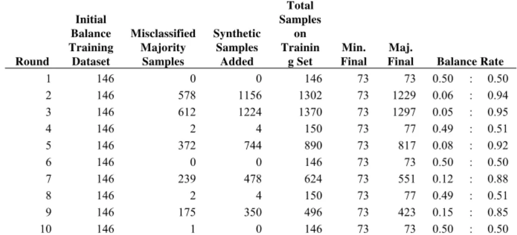
In each round of the algorithm, a new training dataset will be generated. In the first round of the algorithm, the training dataset will be perfectly balanced by under-sampling majority class. From second to the final round, it will also under-sample majority class to start with a balanced training datasets, and additionally new synthetic samples will be generated and added for hard examples on majority class. Table I show an example of 10 rounds of the algorithm for Ozone dataset.

Ozone Dataset has 2536 samples, 73 on minority Class, 2463 on majority class and a balance rate of 0.02:0.98.

TABLE I

GENERATING TRAINING DATASETS ROUNDS FOR OZONE DATASET.

Round

Initial Balance Training Dataset

Misclassified Majority

Samples

Synthetic Samples

Added

Total Samples

on Trainin

g Set

Min. Final

Maj.

Final Balance Rate

1 146 0 0 146 73 73 0.50 : 0.50

2 146 578 1156 1302 73 1229 0.06 : 0.94

3 146 612 1224 1370 73 1297 0.05 : 0.95

4 146 2 4 150 73 77 0.49 : 0.51

5 146 372 744 890 73 817 0.08 : 0.92

6 146 0 0 146 73 73 0.50 : 0.50

7 146 239 478 624 73 551 0.12 : 0.88

8 146 2 4 150 73 77 0.49 : 0.51

9 146 175 350 496 73 423 0.15 : 0.85

10 146 1 0 146 73 73 0.50 : 0.50

As seen to Table I, in some rounds of the algorithm, the balance rate between minority and majority are 50:50. In these cases, it is possible that some samples for majority class will be erroneously classified. To alleviate this loss, the algorithm will generate synthetic samples for these samples in next round. But not matter how many synthetic samples are added in any of the rounds, the balance rate will never larger than the original one 0.02:0.98. This imbalanced reduction will lead to better results on minority class.

III. EXPERIMENTS SETUP

This section will describe the measures and domains used in the experiment.

TABLE II

TWO CLASSES CONFUSION MATRIX

Predicted Positive Predicted Negative Actual

Positive

TP( the number of True Positives

FN (the number of False Negatives) Actual

Negative

FP( the number of False Positives)

TN ( the number of True Negatives) Accuracy, defined as

Acc =

TN FP FN TP

TN TP

+ + +

+ (1)

The TP Rate and FP Rate are calculated as TP/(FN+TP) and FP/(FP+TN). The Precision and Recall are calculated as TP / (TP + FP) and TP / (TP + FN). The F-measure is defined as

(

)

(

1₊β2 _×Recall_×Precision

)(

β2_×Recall₊Precision

)

₍₂₎

Where ß correspond to the relative importance of precision versus the recall and it is usually set to 1. The F-measure incorporates the recall and precision into a single number. It follows that the F-measure is high when both recall and precision are high.

) ( ) (

1

FN TP

TP FP

TN TN where

x mean

g

_a

_a

_a

_a

+ = + = =

− − + − + ₍₃₎

G-mean is based on the recalls on both classes. The benefit of selecting this metric is that it can measure how balanced the combination scheme is. If a classifier is highly biased toward one class (such as the majority class), the G-mean value is low. For example, if a+ = 0 and a− = 1, which means none of the positive examples is identified, g-mean=0 [7].

A. The Receiver Operation Characteristic Curve

A receiver operation characteristic ROC Curve [8] is a graphical approach for displaying the tradeoff between True Positive Rate (TRP) and False Positive Rate (FPR) of a classifier. In an ROC curve, the True Positive Rate (TPR) is plotted along the y axis and the False Positive Rate (FPR) is show on the X axis.

There are several critical points along an ROC curve that have well-known interpretations.

(TPR=0,FPR=0): Model predicts every instance to be a negative class.

(TPR=1,FPR=1): Model predicts every instance to be a positive class.

(TPR=1, FPR=0): The ideal model.

A good classification model should be located as close as possible to the upper left corner of the diagram, while the model which makes random guesses should reside along the main diagonal, connecting the points (TPR=0, FPR=0) and (TPR=1, FPR=1).

The area under the ROC curve (AUC) provides another approach for evaluation which model is better on average. If

the model is perfect, then its area under ROC curve would equal 1. If the model simply performs random guessing, then its area under the ROC curve would equal to 0.5. A model that is strictly better than another would have a large area under the ROC curve.

B. Datasets

The experiments were carried out on 6 real data sets taken from the UCI Machine Learning Database Repository[9] (a summary is given in Table III). All data sets were chosen or transformed into two-class problems.

TABLE III

DATASETS USED IN THE EXPERIMENTS

Dataset Cases Min Class

May Class

Attrib utes

Distributio n

Hepatitis 155 32 123 20 0.20:0.80

Adult 32561 7841 24720 15 0.24:0.76

Pima 768 268 500 9 0.35:0.65

Monk2 169 64 105 6 0.37:0.63

Yeast 483 20 463 8 0.04:0.96

Ozone 2536 73 2463 72 0.02:0.98

Adult dataset training has 32561 examples, but also provides a test dataset with 16281 examples; Monk2 has 169 on training and 432 examples on test dataset. Yeast dataset was learned from classes ‘CYT’ And ‘POX’ as done on [3]. All datasets were chosen for having a high imbalanced degree necessary to apply the method. Minority class was taking as a positive class.

IV. RESULTS AND DISCUSSION

Weka 3.6.0[10] was used as a tool for prediction, C4.5 tree was used as base classifier, AdatabostM1, Bagging, Adacost CSB2, and E-AdSampling were set with 10 iterations.

AdaCost[11]: False Positives receive a greater weight increase than False Negatives and True Positives loss less weights than True Negatives by using a cost adjustment function. A cost adjustment function as:

β

₊=−0.5Cn +0.5 and

β

₋ = 0.5Cn + 0.5 was chosen, where Cn is the misclassification cost of the nth example, and

β

₊ (

β

₋) denotes the output in case of the sample correctly classified (misclassified).

CSB2[11]: Weights of True Positives and True Negatives are decreased equally; False Negatives get more boosted weights than False Positives. Cost factor 2 and 5 were implemented for Adacost and CSB2.

TABLE IV

RESULT COMPARE AGAINST F-MEASURES,TP RATE MIN,ACCURACY, AND G-MEAN.USING C.4.5CLASSIFIER,ADABOOST-M1,BAGGING,ADACOST,

CSB2, AND E-ADSAMPLING ENSEMBLES

Data Set F

Min F Maj TP Rate Min G-Mea n Overall Accu. Hepatitis C4.5 AdaboostM1 Bagging Adacost (2) Adacost(5) CSB2(2) CSB2(5) E-AdSampling 52.8 60.7 51.9 59.7 57.5 60.3 55.0 72.5 90.3 91.3 89.8 88.9 83.4 87.8 75.6 92.1 43.8 53.1 43.8 62.5 78.1 68.8 93.8 78.1 64.2 70.7 63.9 74.0 66.8 76.2 76.1 83.9 83.87% 85.80% 83.22% 82.58% 76.12% 81.29% 68.38% 87.74% Adult C4.5 AdaboostM1 Bagging Adacost(2) Adacost(5) CSB2(2) CSB2(5) E-AdSampling 67.8 64.3 67.1 68.5 64.3 66.7 58.3 70.0 90.9 89.3 91.1 87.4 82.9 87.8 73.8 90.6 62.9 61.9 60.5 82.7 88.2 75.8 95.2 71.0 76.4 75.1 75.3 82.2 80.4 79.8 75.1 80.0 85.84% 83.53% 85.98% 82.02% 76.88% 82.09% 67.79% 85.63% Pima C4.5 AdaboostM1 Bagging Adacost(2) Adacost(5) CSB2(2) CSB2(5) E-AdSampling 61.4 60.6 62.1 61.3 61.5 63.2 57.7 63.5 80.2 78.8 80.3 72.1 65.8 73.3 44.3 81.3 59.7 60.8 60.8 73.5 82.8 76.1 94.0 61.0 69.7 69.1 70.2 68.7 66.6 70.4 52.5 71.3 73.82% 72.39% 74.08% 67.57% 63.80% 69.01% 51.95% 75.26% Monks-2 C4.5 AdaboostM1 Bagging Adacost(2) Adacost(5) CSB2(2) CSB2(5) E-AdSampling 38.9 56.8 48.3 56.3 57.3 56.0 50.0 60.4 75.5 76.6 76.6 58.9 52.1 57.4 4.1 76.9 33.8 60.6 45.8 83.1 92.3 83.8 100 67.6 52.9 67.0 59.9 61.2 58.1 60.3 14.4 69.9 65.04% 69.67% 67.82% 57.63% 54.86% 56.71% 34.25% 70.83% Yeast C4.5 AdaboostM1 Bagging Adacost(2) Adacost(5) CSB2(2) CSB2(5) E-AdSampling 33.3 53.3 0 48.3 47.6 54.5 41.7 61.1 98.3 98.5 97.7 98.4 97.6 98.4 96.9 98.5 20.0 40.0 0 35.0 50.0 45.0 50.0 55.0 44.7 63.1 0 59.0 69.7 66.7 69.3 73.7 96.68% 97.10% 95.41% 96.89% 95.44% 96.89% 94.20% 97.10% Ozone C4.5 AdaboostM1 Bagging Adacost(2) Adacost(5) CSB2(2) CSB2(5) E-AdSampling 23.1 17.2 2.5 26.9 25.7 29.1 26.8 35.3 98.1 98.5 98.4 98.5 97.4 98.3 96.3 98.0 19.2 11.0 1.4 19.2 30.1 23.3 45.2 37.0 43.5 33.0 11.7 43.6 54.0 48.0 65.2 60.1 96.33% 96.96% 96.92% 97.00% 94.99% 96.72% 92.90% 96.09%

In terms of TP Rate measure, compared to non cost-sensitive algorithms, E-AdSampling reduces mistakes in minority class prediction. Take Hepatitis Dataset for example, the difference between E-AdSampling and Adaboost-M1 is 34%. This difference represents a reduction on 8 misclassified cases on minority class. On Ozone dataset, the difference between C4.5 and E-AdSampling is 17.8%, which represents a reduction on 13 misclassified cases on minority class. On these cases or others examples where E-AdSampling performs well, the reduction of misclassified cases on minority class may represent a cost reduction. Compared to cost sensitive algorithms (Adacost, CSB2), E-AdSampling casually would be low for TP Rate minority, but also can be seen how Adacost and CSB2 sacrifice majority class by suffering a reduction on F-measure.

As to F-measure, it is evident how minority class always

obtains an improvement compared to cost-sensitive algorithms as well as non cost-sensitive algorithms. This improving may rise about 12% as on Hepatitis Dataset. For majority class, F-measure is also increased on almost all cases, except for Adult and Ozone datasets where this measure mostly remains constant, just getting a reduction of 0.5. This reduction can be considered small compared to the gain on TP Ratio and F-Measure for minority class.

For the G-mean which is considered as an important measure on imbalanced datasets. E-AdSampling yields the highest G-mean almost on all datasets; except for Adult and Ozone where some cost sensitive algorithms achieve better results. But the results on E-AdSampling show how E-AdSampling can be ideal for imbalanced datasets, indicating also that TP Rate for majority class is not compromise by the increase of TP Rate for minority class.

For the overall accuracy measure, E-AdSampling gets an improving on the 4 datasets. Ozone and Adult are the only Datasets which suffer a reduction. This reduction can be on the range of 1%, which is small compared to the gain on other measures.

As seeen on Table IV Cost-sensitive algorithms (Adacost, CSB2) can achieve good results on TP Rate for minority class. But these results will not be highlighted by reduction on F measures on both class and on some cases a reduction on Overall Accuracy.

Not Cost-sensitive algorithms (C4.5, AdaboostM1, Bagging) only achieve better results for Adult and Ozone Datasets on F-Measure for majority class and Overall Accuracy, E-AdSampling beat this algorithms in others measures.

Fig 3. Roc Curve of the Ozone Data set

To understand better on the achievements of E-AdSampling, a ROC curve for Hepatitis (Fig 2) and Ozone (Fig 3) datasets are presented. Hepatitis dataset was chosen due to the high performance improvement by E-AdSampling and its high imbalanced degree. Ozone dataset was chosen due to the high imbalanced degree and the difficult to classify on minority class. Adacost and CSB2 were executed with Cost factor 2. On both graphics the area under the ROC curve (AUC) show good results for E-AdSampling. Table V show all results for AUC.

TABLE V

Result Area under Curver Hepa

t-itis

Adult Pima Monk s-2

Yeast Ozone

C4.5 AdaboostM1 Bagging Adacost(2) Adacost(5) CSB2(2) CSB2(5) E-AdSampling

0.70 0.81 0.80 0.87 0.83 0.84 0.85 0.88

0.89 0.87 0.90 0.90 0.90 0.89 0.89 0.91

0.75 0.77 0.79 0.78 0.78 0.77 0.78 0.81

0.59 0.73 0.67 0.67 0.69 0.74 0.75 0.71

0.65 0.83 0.79 0.86 0.88 0.86 0.84 0.87

0.67 0.80 0.83 0.83 0.84 0.84 0.83 0.87

V. CONCLUSION

In this paper, an alternative algorithm for imbalanced datasets was presented. Datasets on several and not several imbalanced degree were taking on consideration. In both cases E-AdSampling showed good performance on all measures. Besides E-AdSampling can get good results on TP Ratio and F measure for minority class, it also can remain almost constant or has a slight increase on F-measure for majority class and Overall Accuracy. While some cost-sensitive algorithms gain better results on TP Radio, E-AdSampling can yield better results on F-measures on both majority and minority class as well overall accuracy for almost all cases.

The ROC curves for two of the Datasets, present graphically the achievements of E-AdSampling.

Our future work will be focus on automatically set the number of neighbors needed to generate the synthetics samples and the percent of synthetic samples generated according to the dataset.

ACKNOWLEDGMENT

This paper is supported by the National Science Foundation for Outstanding Youth Scientists of China under Grant No.60425310.

REFERENCES

[1] N. V. Chawla, K. W. Bowyer, and P. W. Kegelmeyer, "Smote: Synthetic minority over-sampling technique," Journal of Artificial Intelligence Research, vol. 16, pp. 321-357, 2002.

[2] N.V Chawla, A. Lazarevic, L.O. Hall, and K.W. Bowyer,

SMOTEBoost: improving prediction of the minority class in boosting. 7th European Conference on Principles and Practice of Knowledge Discovery in Databases, Cavtat-Dubrovnik, Croatia , 107-119, 2003. [3] H. Guo and H. L. Viktor, "Learning from imbalanced data sets with

boosting and data generation: the databoost-im approach," SIGKDD Explor. Newsl., vol. 6, no. 1, pp. 30-39, June 2004.

[4] L. Breiman, "Bagging predictors," Machine Learning, vol. 24, no. 2, pp. 123-140, 1996.

[5] Y. Freund and R. E. Schapire, "A decision-theoretic generalization of on-line learning and an application to boosting," Journal of Computer and System Sciences, vol. 55, no. 1, pp. 119-139, 1997.

[6] J. Han, and M. Kamber, Data Mining: Concepts and Techniques, Elsevier Inc, Singapore, 2006. pp. 360.

[7] R.Yan, Y. Liu, R. Jin, and A. Hauptmann, On predicting rare class with SVM ensemble in scene classification, IEEE International Conference on Acoustics, Speech and Signal Processing (ICASSP'03), April 6-10, 2003.

[8] P. Tan, M. Steinbach, and V. Kumar, Introduction to Data Mining, Pearson Education, Inc, 2006, pp. 220-221.

[9] C.L. Blake and C. J. Merz, UCI Repository of Machine Learning Databases [http://www.ics.uci.edu/~mlearn/MLRepository.html], Department of Information and Computer Science, University of California, Irvine, CA, 1998.

[10] I. H. Witten, and E. Frank, Data Mining: Practical machine learning tools and techniques, 2nd Edition, Morgan Kaufmann, San Francisco, 2005.