Submitted 7 August 2015
Accepted 20 October 2015
Published4 November 2015
Corresponding author Jonathan J. Hudson, [email protected]
Academic editor Jingbo Wang
Additional Information and Declarations can be found on page 15
DOI10.7717/peerj-cs.31 Copyright
2015 Hills et al.
Distributed under
Creative Commons CC-BY 4.0
OPEN ACCESS
An algorithm for discovering
Lagrangians automatically from data
Daniel J.A. Hills, Adrian M. Gr¨utter and Jonathan J. Hudson
Department of Physics, Imperial College of Science, Technology and Medicine, London, United Kingdom
ABSTRACT
An activity fundamental to science is building mathematical models. These models are used to both predict the results of future experiments and gain insight into the structure of the system under study. We present an algorithm that automates the model building process in a scientifically principled way. The algorithm can take ob-served trajectories from a wide variety of mechanical systems and, without any other prior knowledge or tuning of parameters, predict the future evolution of the system. It does this by applying the principle of least action and searching for the simplest Lagrangian that describes the system’s behaviour. By generating this Lagrangian in a human interpretable form, it can also provide insight into the workings of the system.
Subjects Artificial Intelligence, Data Mining and Machine Learning, Scientific Computing and Simulation
Keywords Lagrangian, Physics, Least-action, Discovery
INTRODUCTION
Modern science is, in many senses, highly automated. Experiments are frequently run under computer control, with data often recorded by the computer directly. Computerised data analysis and visualisation are widely used to process the resulting large volumes of data. Indeed, the ability to collect and analyse massive data sets is opening up an entirely new measure-first-ask-questions-later approach to science: the Square Kilometer Array radio telescope is expected to collect approximately one exabyte of data per day (Newman & Tseng, 0000); over 1014collisions from the ATLAS detector were analysed in the search for the Higgs boson (ATLAS collaboration, 2012); and state-of-the-art whole-genome sequencers can currently sequence 600 gigabases per day (Hayden, 2014). In each of these examples the scientific questions are not fully formulated in advance of taking the data, and the question of how to best extract knowledge from the dataset is of great interest. This motivates the study of how to scale up the processes of scientific reasoning to take advantage of the wealth of available data.
Early attempts to automatically model physical systems searched for simple math-ematical regularities in observed quantities.Langley’s (1979) BACON system was able to re-discover many simple laws—the ideal gas law, Ohm’s law, Coulomb’s law and others—from experimental data.Dzeroski & Todorovski (1993)went beyond simple static laws with their LAGRANGE system which was able to search for differential equations that governed observed time series. They extended this work to the LAGRAMGE system which additionally allowed an expert user to provide domain knowledge, improving the quality of the results (Todorovski & Dzeroski, 1997). The PRET system, developed by Bradley and collaborators (2001), brings to bear a variety of advanced AI techniques on the problem of identifying system differential equations. It has a sophisticated method for representing qualitative observations, and allows expert-user domain knowledge to be combined with automatic search very effectively.Schmidt & Lipson (2009)used a genetic programming approach to automatically evolve invariant mathematical expressions from observed data.1
1Note that Schmidt and Lipson originally
claim that their technique is capable of discovering Lagrangians, but it has been shown that this is false except for Lagrangians of a very particular, trivial form (Hillar & Sommer, 2012).Schmidt & Lipson (2010)do not include their claim in a subsequent paper on the same work.
In the context of engineering, there is a significant body of work on ‘system identification’, with techniques ranging from very general ad hoc fitting methods to fitting detailed physical models representing important classes of system (Sjberg et al., 1995;Ljung, 2010).
In this work we take a different approach than those described above, the essence of which is that we embed a simple, general physical principle—the principle of least action—and very little else into our algorithm. While we are embedding the domain knowledge of a physicist in our algorithm, we are not embedding information about any particular physical system or class thereof. Rather we are capturing a deep understanding that has been distilled by physicists over the past 270 years, and packaging it into an algorithm that can be applied by non-experts. We find the algorithm to be surprisingly powerful, given its simplicity, but this power comes not from the ingenuity of its construction, rather from the broad applicability of the physical principle embedded in it.
THE PRINCIPLE OF LEAST ACTION
The principle of least action is one of the most fundamental and most celebrated principles in physics. First proposed byMaupertuis (1744)andEuler (1744)it states that the problem of predicting the behaviour of many physical systems can be cast as finding the behaviour that minimises the expenditure given by some cost function. The total expenditure of the system is known as the action. It is a remarkable fact that the behaviour of a very wide range of physical systems—including those studied in classical mechanics, special and general relativity, quantum field theory, and optics—can all have their behaviour explained in terms of minimising a cost function.
present an algorithm that does this “fiddling” automatically, without requiring the user to have any expertise in physics.
The Lagrangian is well-suited to be the output of an automated modelling algorithm. It has the desirable property in that it is a single, scalar expression that contains everything necessary to predict the system’s future evolution. Consider, in contrast, finding the Hamiltonian where it would also be necessary to find the corresponding conjugate momenta. The Lagrangian has the additional quality that it is coordinate-independent and as a result can be written in any coordinate system. This is useful in the case of an automated algorithm where it is not obvious in which coordinate system the data might be presented. However, it should be noted that not all physical systems can be described by a Lagrangian. In particular, dissipative systems can not be modelled this way. Nevertheless, many interesting processes do admit a Lagrangian formulation, and what’s more, as the algorithm is automatic little is lost by speculatively applying it to a system’s trajectory. We might imagine a future where an ensemble of algorithms such as this one try to find an appropriate model for a system, based on a variety of physical principles and insights. We present this algorithm as a step towards such a future system.
The problem of taking a Lagrangian and automatically calculating the resulting motion of the system has been widely studied and applied. To the best of our knowledge, this work is the first that solves the inverse problem of taking the observed motion and calculating the Lagrangian for non-trivial systems.
THE ALGORITHM
To find a model for a system we search over a space of possible Lagrangians. To do this we need three elements: an objective to guide the search, which will take the form of a score function; a representation of the possible Lagrangians; and an algorithm to execute the search over the possible Lagrangians, working to improve the score. We will first describe the score function, which is the central idea of the algorithm.
Score function
The objective of our algorithm is to find a Lagrangian that, when integrated along the system’s observed trajectory, yields a smaller total (action) than when integrated along any neighbouring trajectory. It would be possible to implement this definition of the least action principle directly in an algorithm, but instead we take an indirect approach that is more computationally efficient. For a LagrangianL(θ ,φ,...,θ ,˙ φ,...)˙ and a trajectory (θ (t),φ (t),...,θ (˙ t),φ(˙ t),...)it is possible to write down a condition, in the form of a set of differential equations, that must be satisfied if the action is to be stationary along the trajectory. These differential equations are known as Euler–Lagrange’s equations,
d dt
∂L ∂q˙ −
∂L ∂q =0,
can define a score function based on these conditions,
EL(L)= q∈{θ ,φ,...}
d dt
∂L
∂q˙ − ∂L
∂q
2
dt, (1)
which is zero if the Euler–Lagrange equations are exactly satisfied. We note that Hillar and Sommer first proposed using a (different) score function derived from the Euler–Lagrange equations inHillar & Sommer (2012), but did not apply it to finding Lagrangians from data.
In practice our observations of the system are not functions(θ (t),φ (t),...,θ (˙ t),φ(˙ t),...) but discretely sampled time-series of the coordinates and generalized velocities. The algorithm operates with a dataset which is a time-series of samples
D=((θ (1),φ (1),...,θ (˙ 1),φ(˙ 1),...),...).
where time runs fromt=1...N. The velocity samples may be either directly measured or derived from measured coordinate data. We divide this time-series into two portions, a training set, comprising samples 1...M, and a validation set of samplesM+1...N. The algorithm will conduct its search using only the training set, reserving the validation set for out-of-sample measurement of the prediction error. In this way we can truly test the algorithm’s ability to predict the future dynamics of the system. In all of the examples in this paper the sampling times will be evenly spaced, but this is not a requirement. We can discretize the Euler–Lagrange score function (Eq. (1)) to work with these sampled datasets, giving
ELD(L)= M
t=1
q∈{θ ,φ,...}
d dt
∂L ∂q˙ t − ∂L ∂q t 2 , (2)
where the subscript on the score indicates that it is taken with respect to the datasetD. The square-bracketed quantities in this expression are time-series, and the subscript indicates taking the element in this time-series at the given time. So, for instance, the first term in (2)is to be calculated, in principle, by: first differentiating the candidate LagrangianL symbolically with respect to the appropriate generalized velocity; evaluating this quantity at every time-step in the dataset to yield a new time-series; taking the discrete derivative of this new time-series with respect to time; and finally finding the element at timetin this time-derivative time-series. In practice, as we shall see below, a more computationally efficient implementation may be used.
introducing a normalisation score for each candidate Lagrangian,
ND(L)= M
t=1
q∈{θ ,φ,...}
d dt
∂L
∂q˙ 2 t + ∂L ∂q 2 t .
We will compose our final score from the scores ELDandNDin such a way, to be detailed below, that to score well a candidate Lagrangian must simultaneously have a low score for ELDand a score of around one forND. The target value of one forNDis chosen arbitrarily. We can always arrange for the normalisation score to be approximately one, as the least-action trajectory is unchanged if the Lagrangian is scaled by a constant.
There is a second, more interesting class, of unwanted expressions that minimise the Euler–Lagrange score ELD. Consider, for instance, the candidate LagrangianL=θnθ˙. This Lagrangian satisfies the Euler–Lagrange equations trivially, in a way that does not depend on the trajectory. Such path-independent least-action Lagrangians are interesting from a physics point-of-view, being closely related to gauge invariance, but here they are a nuisance. To guide the search away from these expressions we introduce a second ‘control’ trajectory,C. This trajectory is unrelated to the behaviour of the system under study and serves solely to eliminate path-independent Lagrangians. We reason that the Lagrangian that we are seeking will score well with ELDbut should score poorly on ELC, which is the
Euler–Lagrange score evaluated along the control trajectory. The exact form of the control trajectory is unimportant so long as it not a valid trajectory of the system under study. In this work we use a control trajectory which is uniform motion in each coordinate, with velocity arbitrarily chosen to be 0.1, for all experiments.
We combine the three parts described above to give the search score function,
S(L)=U(ND(L))U(ELC(L))ELD(L)+ϵ ELC(L)+ϵ
, (3)
whereU(x)=ln(x+ϵ)2+1 is a function that is minimised, with value approximately one, when the argument is one. The small constantϵ, typically set to be 10−10, ensures that the score function has the desired asymptotic behaviour for small values of the numerator and denominator, even when faced with errors from finite precision machine numbers. The factorU(ELC(L))prevents the search algorithm from driving towards Lagrangians that
perform badly on the real dataset, but even worse on the control data. Overall, the score function drives the search to find Lagrangians that simultaneously minimise the action along the observed trajectory while having a non-zero action along the control trajectory, and a normalisation score close to one. We note that the way that the score function is assembled is somewhatad hoc. Its purpose is to guide the search to the correct answer while avoiding pathologies, and there are a number of ways this could be done—indeed, many were tried during development. This score function is simply presented as a particular arrangement that we have demonstrated to work.
on the face of it unrelated, objective leads to successful predictions is the insight from physics that we have embedded in our algorithm.
Representation and search
We have experimented with two representations of candidate Lagrangians. The first, a restricted polynomial representation, allows a fast search algorithm to be implemented. It is limited in the Lagrangians it can represent exactly, although through Taylor’s theorem it can find approximations to any Lagrangian. This representation was used to generate the bulk of the results in this paper, and we describe it in detail in this section. The second representation lifts some of the constraints of the restricted polynomial model, at the expense of vastly increased computational cost. We describe it in ‘Generalisation’.
The restricted polynomial representation assumes that the Lagrangian can be represented by a polynomial in the coordinates and velocities. The model is a sum of monomial terms, parameterised by coefficients multiplying every term. We restrict this polynomial in two ways: we limit the maximum power of any coordinate or velocity to be
m; and we limit the maximum degree of any combination of coordinates and velocities to
p. In addition, we remove any terms from the model that can have no physical significance, that is terms that are constant or of the formqnq˙. These terms simply “fall through” the Euler–Lagrange equation without changing the resulting equations of motion, so there is no value in including them in the search. For example, for one variableθwithm=3 and
p=4 the resulting model would be
c1θ˙2+c2θ˙3+c3θ+c4θθ˙2+c5θθ˙3+c6θ2+c7θ2θ˙2+c8θ3.
For a given restricted polynomial model the score function is minimised by adjusting the parameters ci. We conduct this optimisation using the Nelder–Mead simplex algorithm (Nelder & Mead, 1965) using the modified parameters ofGao & Han (2012)
which improve the efficiency in high dimensions. The coefficients are bounded between −1 and 1, enforced by a penalty function. We use a tight convergence tolerance, usually one part in 1010, to encourage the search to break out of local minima. We impose a maximum iteration limit, usually 5×10⁶, on the search to ensure that it is bounded in time.
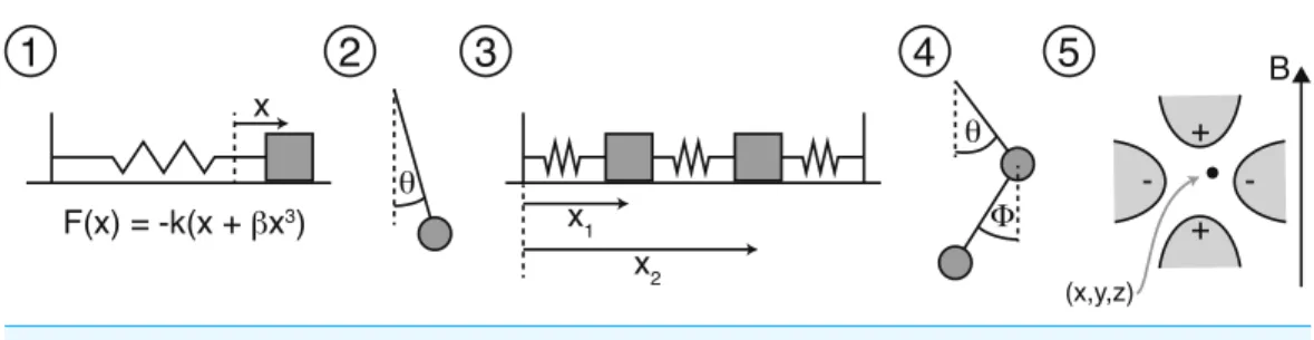
Figure 1 Sketches of the five test systems that we consider.
is found that fits or a maximum bound on model complexity is reached. This heuristic algorithm only crudely captures the notion of mathematical complexity of the model, but it seems to work adequately well.
Note that, for a given polynomial model, it is possible to partially pre-calculate the score function ELDfor a given dataset, yielding a function quadratic in the coefficientsci. This is possible because the form of the model is fixed and it is possible to calculate its derivatives in advance. As a result, after the initial simplification of the score function, optimisation iterations are fast, and have a run-time independent of the number of data points.
Code for the score function, search algorithms and the datasets we use below can be downloaded fromHudson, Hills & Gr¨utter (a).
RESULTS
We will consider five test systems, illustrated inFig. 1. The first is the unforced Duffing oscillator, a textbook non-linear system. The second, a simple pendulum, is interesting because its Lagrangian cannot be represented exactly in the restricted polynomial representation. The third system, two masses on a frictionless surface joined by three springs to each other and two immovable walls, has two coupled degrees of freedom. The fourth system is the double pendulum, a coupled, two degree-of-freedom non-linear system capable of chaotic motion. As with the simple pendulum, the double pendulum cannot have its Lagrangian represented exactly by a finite degree polynomial. The fifth and final system is the Penning-type ion-trap, a three degree-of-freedom system with magnetic and electrostatic forces, that is of considerable experimental relevance.
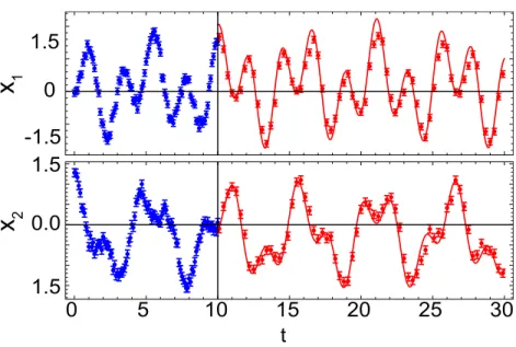
Figure 2shows the result of applying the algorithm to simulated data sets for these
systems. It can be seen that the algorithm is able to successfully predict the future dynamics of all of the test systems. Let us look in detail at the progress of the algorithm, and the resulting learned models, for two of the example systems.
Figure 2 Result of running the algorithm on simulated data from the five test systems.In each graph panel, the (blue) open circles to the left of the vertical bar are the training data. The solid (red) line, to the right of the vertical bar is the algorithm’s prediction. The (red) filled circles to the right of the bar show the actual behaviour of the system. For clarity only every third validation point is shown. The algorithm does not have access to these validation points when it is making its prediction. It can be seen that the algorithm has accurately learned the dynamics of the system in each case.
coefficients to two decimal places for clarity, was
L= −0.30x2+0.14x4+0.20x˙2.
Figure 3 Application of the algorithm to data with simulated noise added.The graphs are in the same format asFig. 2. We see that the algorithm is robust to noise, finding a model that accurately predicts the future evolution.
coefficients to the 6th decimal place, limited by the convergence tolerance that we set. By generating a model in this form the algorithm gives insight into the system directly from the data.
The case of the simple pendulum is also interesting to consider. Here the search algorithm tried three models, where the third, withm=2 andp=4, converged in 480 Nelder–Mead iterations. The search in this case took around 0.6 s. The generated model, multiplied by 100 to make it more readable, was
L=0.049x+8.6x2−3.0x˙2−0.0030xx˙2 −0.41x2x˙2. (4)
It can be noted that this is not a straightforward Taylor expansion of the simple pendulum’s Lagrangian, and it is not obvious how to relate it to the standard form. Experimenting with removing terms and solving the resultant equations of motion indicates that the terms proportional toxandxx˙2are unimportant, but the relatively small term inx2x˙2is essential. Despite being in an unexpected form, this Lagrangian does make successful predictions. We shall see in ‘Generalisation’ that it is in fact a local approximation of a true Lagrangian around the region of configuration space that the training trajectory explored.
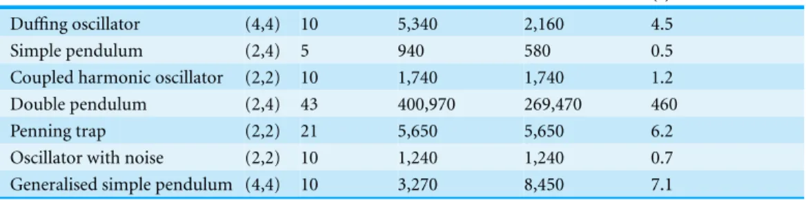
Table 1 Summary of models found for each of the test systems and the computational effort required to find them.“Total iterations” gives the number of Nelder–Mead iterations used searching through all forms of the model, including the final form. “Final iterations” gives the number of Nelder–Mead itera-tions used refining the final form of the model. The “Generalised simple pendulum” will be introduced in ‘Generalisation’.
System (m,p) Parameters Total iterations Final iterations Time to converge (s)
Duffing oscillator (4,4) 10 5,340 2,160 4.5
Simple pendulum (2,4) 5 940 580 0.5
Coupled harmonic oscillator (2,2) 10 1,740 1,740 1.2
Double pendulum (2,4) 43 400,970 269,470 460
Penning trap (2,2) 21 5,650 5,650 6.2
Oscillator with noise (2,2) 10 1,240 1,240 0.7
Generalised simple pendulum (4,4) 10 3,270 8,450 7.1
Table 1summarises the size of the models found and the computational effort required
to find them. We have not conducted a detailed study of how this proof-of-principle algorithm scales as the problem size increases, but note that our preliminary investigations show that it scales quite poorly. We find that the primary determinant of convergence rate seems to be the number of free parameters in the model. We therefore speculate that a more sophisticated technique for varying the structure of the model might be of use in improving the performance. A particularly promising approach might be to follow (Clegg et al., 2005) and use a genetic algorithm to evolve the form of the model in combination with a continuous algorithm like Nelder–Mead to optimise the parameter values for any given model form.
GENERALISATION
We have shown that the algorithm can find models which successfully predict the future evolution of the system’s behaviour. However, a good physical model does not just capture the behaviour of a particular time-series, corresponding to a particular set of initial conditions. Rather, it should be able to predict the behaviour of the system over a range of initial conditions. It is perhaps this ability to generalise that sets a true physical model apart from a mere fit or interpolation of the system’s behaviour. It is interesting, therefore, to study whether the models found by our algorithm have this property.
We have seen in the case of the Duffing oscillator that the discovered model is indeed the correct model, and we would expect that this model will correctly predict the dynamics of the system for any initial conditions. We test this by simulating the behaviour of the system for a wide range of initial conditions, and comparing the results to the predictions of the model. We find, as expected, that the learned model for the Duffing oscillator does make correct predictions for all initial conditions.
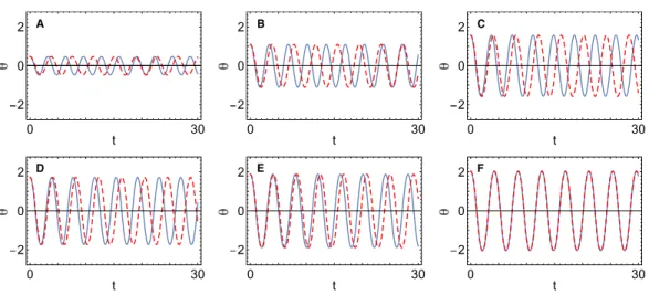
Figure 4 Predictions for different initial conditions of the learned simple pendulum model (red dashed line) compared to the true behaviour (blue solid line).The amplitude of the pendulum swing varies between panels. The model was trained at the amplitude shown in (F). We see that the model makes good predictions for the initial conditions it was trained on, but breaks down for other initial conditions.
sophisticated curve fitting routine, but rather is finding the underlying physical truth behind the system dynamics to make its predictions.
The pendulum and double pendulum models do not generalise well, as we might have anticipated from the form of the Lagrangian inEq. (4).Figure 4 compares the prediction of the learned simple pendulum model against the true behaviour, for a variety of swing amplitudes. We see that while the prediction is accurate for the amplitude at which the model was trained, it deviates at other amplitudes. These results are perhaps to be expected, and could well be the same as generated by a human physicist given the same data. The algorithm has found a mathematically simple approximation that works well for the data it has available to it, but does not have enough to go on to determine the true underlying model.
We consider two approaches to generating models that generalise better for these systems, inspired by the approaches a human physicist might take. The first method is simply to train the models with more data, corresponding to a wider range of initial conditions. The second is to introduce new mathematical constructs which allow a simpler model to be found, reasoning that this model is more likely to generalise well.
For the first approach we follow exactly the same procedure as before except we generate a number of trajectories, corresponding to a range of initial conditions, and use a score that is the sum of the scores for the individual trajectories. We applied this procedure to the simple pendulum system. The resulting search takes approximately 15 times longer to converge than the single-trajectory search. We find that the algorithm is unable to converge on anm=2,p=4 model, as it did before, and has to continue its search until it finds anm=4,p=4 model whose predictions fit all of the trajectories adequately.
Figure 5compares the predictive ability of this model with the ‘single-trajectory’ model
Figure 5 Comparing a model for the simple pendulum trained on multiple trajectories with one trained on a single trajectory.The curves show the squared error between the model’s prediction and the true behaviour, as a function of the pendulum’s swing amplitude. The dashed (blue) curve shows the result for a model trained at a single swing amplitude, indicated by the heavy (blue) arrow. This model performs well at the amplitude it was trained at, but poorly at other amplitudes. The model corresponding to the solid (red) curve was trained with multiple trajectories, indicated by the other (red) arrows. The original trajectory was also included in the training set for this model. We see that the ‘multi-trajectory’ model makes better predictions across a wide range of initial conditions, including conditions that it was not trained on. The multi-trajectory model is able to make successful predictions up to surprisingly large amplitudes, well beyond those it has seen in training.
good predictions for the initial condition it was trained at, but makes poor predictions for other initial conditions. The ‘multi-trajectory’ model, though, is much improved. It makes good predictions at all of the initial conditions it was trained at, and further makes good predictions at other, unseen initial conditions as well. We have found similar results for the double-pendulum system, although the computational expense of the problem constrained the experiment to a limited region of initial-condition-space.
Our second approach to generalisation is to expand the representation of the Lagrangians to encompass a wider range of mathematical expressions. We reason that, with a wider palette of mathematics at its disposal, the algorithm may be able to find a model of simpler form that works well. History has shown, although this may be tautological, that often systems of interest to physicists can be described by remarkably simple mathematical models. We hope that by allowing the algorithm to generate structurally simpler models, it may be more likely to discover the underlying physical truth.
an algorithm (Zitzler, Laumanns & Thiele, 2001) that simultaneously tries to optimise the score and minimise the size of the trees. Thus, this search algorithm tries explicitly to find simple expressions that score well on the data.
Repeating the search on large-amplitude (±0.95π) simple pendulum data using the tree-based representation highlights the relative strength of this approach. The generated model, which makes a successful prediction, is
L=0.25θ˙2+2.0cos(θ ),
the same as would be written by a human physicist. Naturally, this model makes correct predictions over the full range of initial conditions. There are two reasons that the tree-based expression search is able to converge on this model. First it is only because the representation of possible models is richer that this model can be directly represented at all. Second, the notion of mathematical complexity in this representation more closely models that of a human physicist. This allows the search algorithm to do more work driving the result towards an expression that we recognize as canonical. It must be cautioned, though, that this is only a proof-of-principle demonstration. To reach this result we had to bias the search algorithm, as described in theAppendix, and even then the run time is significantly longer, often taking many hours with a multi-threaded implementation on the hardware described above. We were not able to get results for the double pendulum system at all with the computing resources at our disposal. Nonetheless, we present this result as the technique shows potential for learning models that are both better able to generalise, and in a format more suitable for communication to human physicists.
CONCLUSION
We have demonstrated an algorithm that can predict the future dynamics of a physical system directly from observed data. We have shown that the algorithm generates models that can be communicated to a human physicist, sometimes even finding models in textbook form. We have further shown that the models generated generalise well to unseen data, and are not merely fits or interpolations, but are truly capturing the physical essence of the system under study.
One might ask what the use of such an algorithm is. As a first point, we find the question of whether a computer can do science to be fascinating in itself. Investigating the limits of a computer’s ability in this regard educates us as to the strengths and weaknesses of our current scientific processes, and invites us to consider a different perspective on our scientific work.
Figure 6 An expression tree representingθ2−3cos(θ )˙ .
non-specialists. By capturing the idea of searching for least action models in an algorithm we make it available to anyone, including those without the necessary skills to do it by hand. By way of analogy, it is interesting to consider popular online natural language translation software. While no-one would consider these tools suitable for translating poetry, they nonetheless are exceedingly useful to many people in the common case where a ‘good-enough’ translation will do. While we do not imagine computers will replace expert human physicists in the near term, we envisage the availability of tools to automate scientific reasoning will empower non-specialists to take better advantage of the discoveries and insights of physics.
ACKNOWLEDGEMENTS
We acknowledge many useful discussions with Jeremy Mabbitt, Mike Tarbutt, Jack Devlin, Iain Barr, Ben Sauer, and Ed Hinds. DJAH and AMG contributed equally to this work.
APPENDIX: TREE-BASED REPRESENTATION AND
SEARCH
Here we describe in detail the tree-structured symbolic representation of mathematical expressions and the corresponding search routine. The expressions are built following a grammar designed to bias the search towards expressions that might be Lagrangians for simple physical systems. Each terminal of these expression trees is one of: numerical constants, randomly generated; the coordinate variables and velocities; the squares of the coordinates and velocities; and for coordinates which represent angles, the sine and cosine of the coordinates and velocities. The non-terminal nodes of the trees are the operators +,−,×. An example expression tree is shown inFig. 6, representing the expression θ2−3cos(θ )˙ .
In detail, we first construct a population of randomly generated expressions, usually numbering 100. We score these expressions using the least-action score and also assign a complexity score which is simply the number of nodes in the expression tree. The SPEA2 algorithm takes the current population, and an initially empty set of elite expressions, representing the best that have been seen so far. It has a rather complex selection mechanism (Zitzler, Laumanns & Thiele, 2001) that produces a new set of elite expressions, plus a set of expressions, the breeding pool, which are candidates for reproduction. A new generation is created from the breeding pool by mutation (10%) and pair-wise crossover (90%). Mutation is effected by replacing a randomly chosen subtree of the given expression with a randomly generated subtree. The crossover operation takes two expressions, selects a random point in each of the two trees, and swaps the sub-trees at these points to generate two new expressions. The evolutionary process is repeated starting from this new generation, and we iterate for a large number of generations, typically many thousand. To improve the convergence speed of the numeric constants in the expressions we also incorporate a small amount of hill-descent into each evolutionary iteration: a subset (20%) of the expressions have their numeric constants randomly adjusted by a small amount, and if this improves their least-action score, the modification is kept. We also impose a maximum size of expression (50 nodes) and trim expressions that exceed it each generation to ensure that the run-time is bounded. The final elite set is a set of expressions that represent the trade-offbetween least-action score and complexity. We select from this set the simplest expression that has a least-action error below a specified threshold.
In this tree-based method, the structure of the candidate Lagrangians varies during the search, so it is not possible to partially pre-calculate the score function, as it was in the restricted polynomial technique. Rather it must be calculated in full for each expression in the population. Further, the search space of possible expressions is exceedingly large, and the score is not very smooth with respect to the genetic operations. As a result, the search must run for many generations and is extremely computationally expensive. A na¨ıve implementation might calculate the partial derivative time-series in (Eq. (3)) by symbolically differentiating the candidate expression and then calculating the value of the derivative. This, however, can be exponentially expensive in the depth of the expression, in terms of both memory and runtime. A better approach, that we adopt in this work, is to simultaneously evaluate the expression’s value and its derivatives using automatic differentiation (Kalman, 2002). This method avoids calculating an expression for the derivative, and has run-time proportional to the size of the expression.
ADDITIONAL INFORMATION AND DECLARATIONS
Funding
The authors received no funding for this work.
Competing Interests
Author Contributions
• Daniel J.A. Hills and Adrian M. Gr¨utter performed the experiments, analyzed the data, performed the computation work, reviewed drafts of the paper.
• Jonathan J. Hudson conceived and designed the experiments, performed the experi-ments, analyzed the data, contributed reagents/materials/analysis tools, wrote the paper, prepared figures and/or tables, performed the computation work, reviewed drafts of the paper.
Data Availability
The following information was supplied regarding data availability:
https://github.com/JonyEpsilon/flow.
REFERENCES
ATLAS collaboration. 2012. Observation of a new particle in the search for the
Standard Model Higgs boson with the ATLAS detector at the LHC. Physics Letters B
716:1DOI 10.1016/j.physletb.2012.08.020.
Bradley E, Easley M, Stolle R. 2001.Reasoning about nonlinear system identification.Artificial Intelligence133:139DOI 10.1016/S0004-3702(01)00143-6.
Clegg J, Dawson J, Porter S, Barley M. 2005.The use of a genetic algorithm to optimize the functional form of a multi-dimensional polynomial fit to experimental data.The 2005 IEEE congress on Evolutionary computation1:928–934DOI 10.1109/CEC.2005.1554782.
Dzeroski S, Todorovski L. 1993.Discovering dynamics. In:Proc. tenth international conference on machine learning. San Mateo: Morgan Kaufmann Publishers Inc., 97–103.
Euler L. 1744.Methodus inveniendi lineas curvas maximi minive proprietate gaudentes.
In:Methodus inveniendi lineas curvas maximi minive proprietate gaudentes. Bousquet, Lausanne & Geneva.
Feynman R, Leighton R, Sands M. 1963.The Feynman lectures on physics. In:The Feynman
lectures on physics. 2nd edition. vol. 1. Boston: Addison-Wesley.
Gao F, Han L. 2012.Implementing the Nelder-Mead simplex algorithm with adaptive parameters.
Computational Optimization and Applications51:259DOI 10.1007/s10589-010-9329-3.
Hayden EC. 2014.Is the $1,000 genome for real?NatureDOI 10.1038/nature.2014.14530.
Hillar C, Sommer F. 2012.Comment on the article “Distilling free-form natural laws from
experimental data”. ArXiv preprint.arXiv:1210.7273.
Hudson JJ, Hills DJA, Gr¨utter AM.Flow project code.Available athttps://github.com/JonyEpsilon/ flow.
Kalman D. 2002.Doubly recursive multivariate automatic differentiation.Mathematics Magazine
75:187DOI 10.2307/3219241.
Koza JR. 1992.Genetic programming: on the programming of computers by means of natural
selection. Cambridge: MIT Press.
Langley P. 1979.Rediscovering physics with BACON.3. In:Proceedings of the 6th international joint conference on artificial intelligence. vol. 1. San Francisco: Morgan Kaufmann Publishers Inc., 505–507 series and number IJCAI’79.
Ljung L. 2010.Perspectives on system identification.Annual Reviews in Control34(1):1–12
Maupertuis PLM De. 1744.Accord de diff´erentes lois de la nature qui avaient jusqu’ici paru incompatibles.M´em. As. Sc. Paris417.
Nelder JA, Mead R. 1965.A simplex method for function minimization.The Computer Journal
7(4):308–313DOI 10.1093/comjnl/7.4.308.
Newman R, Tseng J.Memo 134: cloud computing and the square kilometre array.Available at
http://www.skatelescope.org/uploaded/8762 134 Memo Newman.pdf.
Schmidt M, Lipson H. 2009.Distilling free-form natural laws from experimental data.Science
324(5923):81–85DOI 10.1126/science.1165893.
Schmidt M, Lipson H. 2010.Symbolic regression of implicit equations. In: Riolo R, O’Reilly U-M, McConaghy T, eds.Genetic programming theory and practice VII, genetic and evolutionary computation,Genetic and evolutionary computation.Springer, 73–85.
Sj¨oberg J, Zhang Q, Ljung L, Benveniste A, Delyon B, Glorennec P-Y, Hjalmarsson H, Judit-sky A. 1995.Nonlinear black-box modeling in system identification: a unified overview. Trends in System Identification,Automatica31(12):1691–1724DOI 10.1016/0005-1098(95)00120-8.
Todorovski L, Dzeroski S. 1997.Declarative bias in equation discovery. In:Proc. fourteenth international conference on machine learning. San Mateo: Morgan Kaufmann Publishers Inc., 376–384.
Zitzler E, Laumanns M, Thiele L. 2002.Giannakoglou K, et al., ed.Evolutionary methods