Developing a Forecasting Analysis Framework to Fast Track Analytical Developments

F

E

U

P

Developing a Forecasting Analysis

Framework to Fast Track Analytical

Developments

Verónica Sofia Marcos Fradique

Mestrado Integrado em Engenharia Informática e Computação Supervisor: Prof. José Luís Borges

Developing a Forecasting Analysis Framework to Fast

Track Analytical Developments

Verónica Sofia Marcos Fradique

Mestrado Integrado em Engenharia Informática e Computação

Approved in oral examination by the committee:

Chair: Prof. João Moreira

External Examiner: Prof. João Vinagre Supervisor: Prof. José Luís Borges

Abstract

Digitalization is an emerging concept and is increasingly getting relevance among companies. Due to this, some companies realize a need to change their own business models, in order to adapt to market impositions and requirements. One of the most important factors in this process is the reduction of lead times. To achieve this, it is necessary to create an environment integrating all the conditions to allow fast development and deployment of the solutions.

Forecasting plays a pivotal role in several industries that deal with uncertainties in the global and domestic markets. It helps in different domains, from business operations optimization to anticipating changes in the markets. In the context of LTPlabs, a boutique consultancy company that develops data-driven solutions to assist clients in making better decisions, forecasting is a typ-ical problem being addressed daily. When a forecasting project starts, the business requirements and needs are defined. Then data is collected among the different sources, cleaned from missing values, and analyzed to understand it in terms of overall statistical analysis. After this process, data is selected and prepared to start forecasting. The next two steps are to select a forecasting algorithm and evaluate its performance. The process is iterative until a satisfactory evaluation is accomplished, proceeding to the deployment of the solution. Across projects, there are implemen-tations of tools that support preprocessing, forecasting algorithms, and evaluation metrics that are not being reused since they are tailored to the specific project’s data.

Actual forecasting performance, already achieved with the forecasting techniques used, and how they are chosen and tested, can be leveraged with a high-level framework aggregating the most common and some state-of-the-art techniques and evaluation metrics as well as preprocessing tools. In the reviewed literature, there is not a tool able to answer the identified needs, providing a fast analysis with lower user inputs and, at the same time, able to customize it to control and track all the stages of the development. Aiming to achieve better forecasting results and address a wider range of projects, an automatic approach to forecast was proposed and a framework developed including, also, grouped structure forecasting and inclusion of exogenous variables.

The high-level framework developed was tested with analysts on ongoing projects and was easily accepted and adopted, leading to a significant reduction in development times. Additional side effects include reducing costs maintaining and improving the high quality of the solutions developed and deployed. Moreover, the standardization of the forecasting process throughout the company, and systematization of existing knowledge related to the topic result from the imple-mentation of the framework, ensuring quicker and easier access to main forecasting techniques.

Keywords: Forecasting, Hierarchical Forecasting, Grouped Forecasting

Resumo

A digitalização é um conceito emergente e cada vez mais presente no quotidiano das empresas. Para acompanhar este ciclo de mudança, várias empresas veem-se na necessidade de alterar os seus modelos de negócio, adaptando-se, assim, às novas necessidades e imposições do mercado. Um dos principais fatores tidos em conta nesta mudança é a redução do tempo que decorre entre o pedido do cliente e a entrega da solução personalizada que satisfaz as suas necessidades. Para tornar este processo mais rápido, é necessário criar um ambiente com as condições adequadas para permitir um rápido desenvolvimento.

A previsão é uma componente importante em diversas empresas, de diferentes setores que lidam com fatores de incerteza no mercado. A previsão permite o auxílio a diferentes niveis, desde a otimização da operações internas, até à previsão estimada de vendas, antecipando as tendências nos mercados.

No contexto específico da LTPlabs, uma empresa que desenvolve soluções analíticas para apoiar clientes na tomada de decisões mais informadas, as previsões estão presentes diariamente. Quando se inicia um projeto, definem-se as necessidades do negócio e os seus objetivos. Após isto, os dados são recolhidos e analisados estatisticamente, de uma forma global. Seguidamente, são selecionados e preparados para dar início ao processo de previsão. As duas fases seguintes consistem em escolher um algoritmo, implementá-lo e avaliar a sua performance. Este processo segue iterativamente até o resultado da fase de avaliação ser favorável, passando, assim, à im-plementação da solução final. De projeto para projeto, há implementações de ferramentas de pré processamento dos dados, algoritmos e métricas de avaliação que não são reutilizadas por estarem demasiado adapatadas aos dados de cada projeto específico.

Na revisão de literatura efetuada, não se encontrou nenhuma ferramenta capaz de responder às necessidades identificadas, providenciando uma análise rápida, com um número diminuto de comandos introduzidos pelo utilizador, e, ao mesmo tempo, personalizável para controlar e mon-itorizar todas as etapas do processo de previsão. Assim, foi proposta uma abordagem automática para o processo e desenvolvida uma ferramenta, incluindo ainda estruturas agrupadas e previsões com variáveis exógenas.

A ferramenta desenvolvida foi testada com analistas no decurso dos seus projetos, tendo sido aceite e incorporada nas metodologias, levando a uma melhoria significativa dos tempos desen-volvimento. Com isto, espera-se uma redução dos custos, assim como um aumento da quali-dade das soluções desenvolvidas e implementadas. Em acréscimo, destacam-se as melhorias na padronização do processo de desenvolvimento de previsões, bem como na sistematização do con-hecimento relacionado com o tema, permitindo um acesso fácil e rápido às principais técnicas de previsão.

Keywords: Previsão, Previsão Hierárquica

Acknowledgements

Que viagem! É esta a sensação ao olhar para os últimos 5 anos! Não é o fim que imaginei, se é que alguma vez imaginara o final disto. Não sei se levo os melhores 5 anos da minha vida neste pedaço de história, mas levo anos incríveis! Não podia estar mais grata a todos os que me ajudaram a chegar até aqui! Cá estamos, conseguimos!

Obrigada à LTPlabs pela oportunidade de passar os últimos meses a contribuir para um projeto tão ambicioso, numa equipa incrível, rodeada de pessoas sempre à procura de fazer mais e melhor! Obrigada ao Francisco Amorim por todo o apoio e por ter partilhado tanto do que sabe! Sem dúvida que foi essencial para tudo o que aprendi e para toda a dissertação.

Obrigada ao João Alves pela forma como me acompanhou ao longo desta dissertação, estando sempre disposto a esclarecer todas as dúvidas.

Obrigada ao Professor José Luís Borges, pela disponibilidade e apoio ao longo de todo este período, contribuindo sempre com valiosos conselhos.

Obrigada a todos os amigos que me acompanharam ao longo do percurso. Poder contar con-vosco, partilhar experiências e criar memórias é, definitivamente, incrível!

Obrigada à família por terem estado sempre lá! Sem dúvida que são o meu pilar em todas as etapas e esta conquista também é vossa! Obrigada à minha irmã por ser a minha inspiração e a minha motivação, em todas as alturas. Obrigada à minha mãe por ser o porto seguro, pelo apoio incondicional e por viver comigo todos os momentos. Obrigada ao meu pai por toda a motivação e por me incentivar sempre a desafiar os limites e a deixar a zona de conforto bem distante!

Obrigada ao João por todo o apoio, por toda a motivação e por termos vivido tanto ao longo destes anos.

Verónica Fradique

“She stood in the storm and when the wind did not blow her way, she adjusted her sails.”

Elizabeth Edwards

Contents

2.1.1 Naïve and classical forecasting methods . . . 6

2.1.2 Machine learning applied to forecasting . . . 8

2.1.3 Ensemble techniques . . . 9

2.1.4 Algorithm selection . . . 10

2.1.5 Hierarchical structure . . . 11

2.2 Diagnosis and classification . . . 11

2.3 Evaluation metrics . . . 13

2.4 Technologies . . . 15

2.5 Exogenous variables in forecasts . . . 16

2.6 Summary . . . 17

3 Problem Description 19 3.1 Current forecasting approach . . . 19

3.2 Forecasting application . . . 21

3.3 Proposed approach . . . 22

4 Methodology 25 4.1 Proposed approach . . . 25

4.2 Structure and information organization . . . 26

4.3 Diagnosis tools integration . . . 29

4.4 Classifications’ integration . . . 29

4.5 Evaluation metrics’ integration . . . 30

4.6 Algorithms integration . . . 30

4.6.1 Naïve algorithms . . . 30

4.6.2 Classical algorithms from R Forecast package . . . 31

4.6.3 Ensemble methods . . . 32

4.7 Exogenous variables integration . . . 33

4.8 Grouped forecasting . . . 34

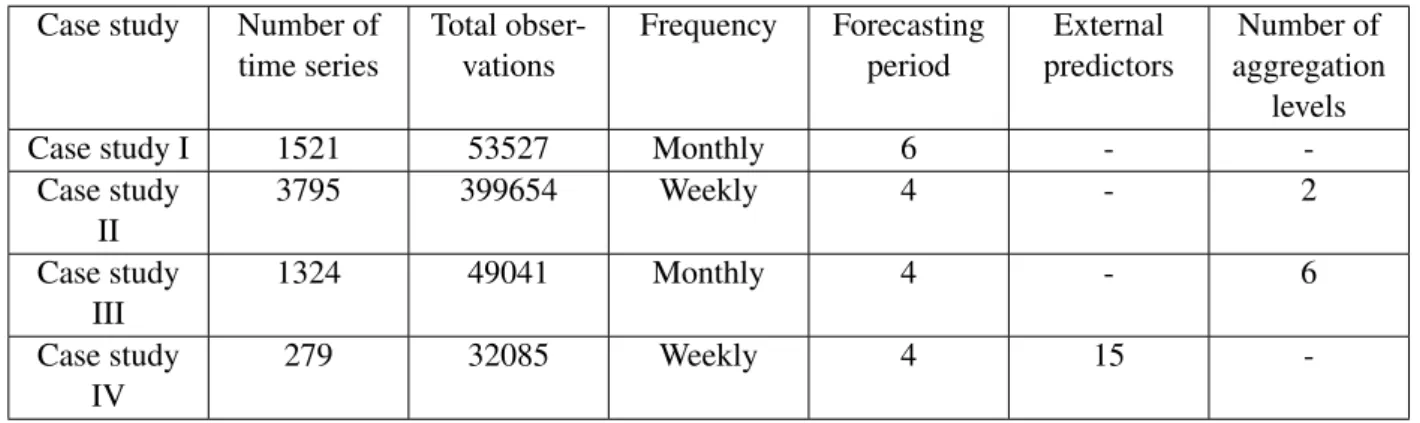
5 Results 37 5.1 Case studies description . . . 37

5.2 Lead times impact . . . 38

x CONTENTS

5.3 High-level framework . . . 40

5.3.1 Introduction to forecasting basics . . . 40

5.3.2 Grouped forecasting . . . 45

5.4 Case study overview . . . 46

6 Conclusions 51 6.1 Implications for practice . . . 51

6.2 Future work . . . 52

A Complete evaluation metrics table 55

List of Figures

2.1 Example of time series non stationary and stationary. . . 7

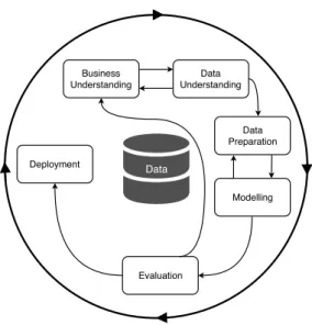
2.2 Graphical representation of demand in each category of SEIL classification, [26]. 13 3.1 The CRISP-DM process model of data mining, still applied to forecasting. . . 20

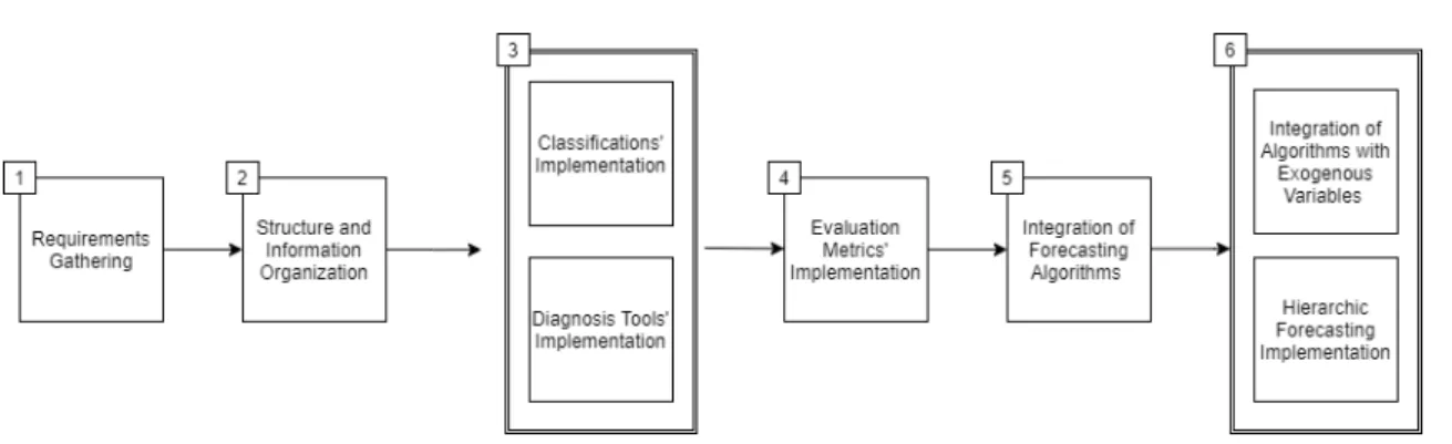
4.1 Proposed development approach of the framework. . . 26

4.2 Framework interactions. . . 27

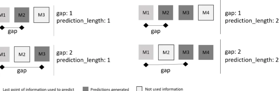
4.3 Interaction between gap and prediction length. . . 28

5.1 Comparison between previous forecasting projects duration and current approach. 39 5.2 ABC analysis plot. . . 42

5.3 Percentage of X, Y and Z in each ABC categories. . . 42

5.4 Outliers plot through IQR method. . . 43

5.5 Part of evaluation metrics table provided by the framework. . . 44

5.6 Evaluation of forecasts in terms of MAPE and Bias in classifications ABC and XYZ. 45 5.7 Evaluation metrics per level and model with gradient color from dark red (worst) to green (best). The blank spaces refer to ML algorithms which have a minimum of 20 items per model. . . 47

5.8 Evaluation metrics on case study III, with grouped forecasting. . . 48

A.1 Comparison between previous forecasting projects duration and current approach. 56

List of Tables

2.1 Example of first order differencing. . . 6

2.2 Evaluation Metrics . . . 14

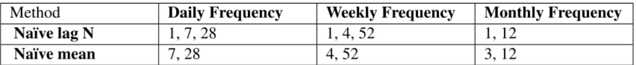
4.1 Default parameters for Naïve methods, according to time series frequency. . . 31

5.1 Case studies characteristics. . . 37

5.2 Case Studies execution times. . . 40

5.3 Forecasting results of case studies I, II and IV. . . 48

Abbreviations

ADI Average Demand Interval

ARIMA Autoregressive Integrated Moving Average CRISP-DM Cross-Industry Standard Process for Data Mining CV2 Squared Coefficient of Variation

GBM Gradient Boosting Machine MAE Mean Absolute Error

MAPE Mean Absolute Percentage Error MASE Mean Absolute Scaled Error ML Machine Learning

NN Neural Networks pp Percentage Points

RMSE Root Mean Squared Error

SARIMAX Seasonal Autoregressive Integrated Moving Average with exogenous variables SMA Simple Moving Average

Chapter 1

Introduction

Increased competitiveness is a trend spreading in the last decades across several industries. Cus-tomers demand better service levels, companies press suppliers for decreased lead times and brand loyalty is not what it was a few years ago.

A fundamental interest in deploying an effective data-driven decision-making framework is having general knowledge on how the future is going to play out, regarding some key business variables such as sales, stock consumption and even to understand where is the best place to spot the next company building.

1.1

Context

The forecasting process is hard and consuming an increased quantity of resources, human and computational, for long periods. In business consultancy companies, a substantial part of the projects is associated with forecasting.

This project was conducted with LTPlabs, a Portuguese consultancy company that creates data-driven solutions to leverage clients’ procedures in a vast area. Most of the projects this company develops are forecasting projects or other domain projects that require a forecasting module to support some part of them.

The methodology the company adopted, formally or informally, to overcome the challenges of each forecasting process is Cross-Industry Standard Process for Data Mining (CRISP-DM). This methodology divides the forecasting projects into six distinct phases, that are highly correlated with each other. Succinctly describing each step of CRISP-DM:

• Business understanding covers the familiarization with forecasting problems, being the cru-cial point to understand the goals and to define requirements from a business perspective; • Data understanding consists of collect, clean and standardize data as well as explore it across

different analysis, being an enduring task; 1

2 Introduction

• Data preparation focus is on the definition of the final data structure with all the relevant information;

• Modelling consists of the selection of an algorithm to use as the forecasting strategy and its parameters;

• Evaluation comprises critically analyzing the results obtained previously. When the results addressed in the last phase are satisfactory to meet business needs, the algorithm under analysis is deployed and the forecasting process is complete.

In each project developed, the first and the last phases are unique since they depend on spe-cific business needs and requirements. However, remain four phases are similar independently of the project nature: understanding data, statistically, preparing it, choosing an algorithm, and evaluating it. From a consultancy company’s perspective, after each project developed, there are implementations of algorithms, data analysis tools, and evaluation metrics that are not being reused and, consequently, developed multiple times. It leads to previously acquired knowledge that is not being properly used if that are just some users managing it, from an organization’s point of view.

In the reviewed literature it was not found a solution to allow a forecasting analysis from end to end with a reduced set of commands. In the market, there several solutions, such as Forecast Pro, [21], that provide support to a significant part of the forecast analysis but are not open source. To combine the knowledge previously acquired by the company, such as recommended strategies, algorithms, or even evaluation metrics, the existence of a framework developed and implemented from the beginning is important, to allow its expansion to adapt to their needs.

Aiming to combine a plethora of algorithms, data analysis tools, and evaluation metrics in a single framework the main goal set for this project is to reduce forecasting projects lead times. Along with this main goal, comes a set of issues that are addressed in the process, as the stan-dardization of steps followed to forecast, an increase of the number of algorithms tested, and systematization of different techniques and knowledge acquired that remain accessible in a single point, reducing the programming needed by providing a high-level framework.

To cover a wide spectrum of projects, it is important to gear the framework with the most used and some state-of-the-art algorithms, a set of tools to help data diagnosis, and a vast quantity of evaluation metrics. Also, the interpretation of a hierarchical structure of data and best level selection as well as the inclusion of exogenous variables, since they can lead to higher accuracy of the forecasts, are included.

To address the advantages and the impact of a framework as the one briefly summarized, there are four case studies to clearly state the reduction of development times, the diminished programming skills required to implement an end to end forecast and simulation of an analyst interpretation of the framework output.

1.2

Dissertation structure

1.2 Dissertation structure 3

The present chapter introduced the project, contextualized the problem and the main goals are stated.

Chapter2is dedicated to providing an overview over a wide range of forecasting techniques along with a discussion of the complementary needs to give support both to forecasting and im-plementation.

Chapter3describes in detail the current methodology used, the main drawbacks of it as well as a brief description of the proposed approach.

Chapter 4 details the previous proposed methodology. It covers the initial structure of the information, the implementation, and the integration of different tools, algorithms, grouped fore-casting, and exogenous variables inclusion.

Then, in chapter5the results of the implementation are presented and discussed based on the analysis of four case studies.

Concluding, chapter 6 draws the main conclusions of the project alongside a set of future guidelines for improvements.

Chapter 2

Literature Review

The present chapter aims to provide a general overview of the forecasting techniques available, data analysis tools, evaluation metrics, and implementation. Section2.1 introduces forecasting techniques from simple to complex ones and addresses the challenges in the selection of the most adequate for a given problem. Data diagnosis tools and data classifications to assess time series characteristics are presented in section2.2. In section2.3 the evaluation metrics to obtain a sta-tistical performance of the forecasts are described. To address the implementation of the concepts of the previous section, in section 2.4 technologies are discussed. To complete the forecasting overview, a review of the usage of exogenous variables is described in section2.5. The chapter concludes with a summary of the main topics discussed, in2.6.

2.1

Forecasting techniques

Forecasting is an extensive topic and can be used in a wide range of contexts. During this chapter, the term forecasting is applied to time series forecasting. Time series consists of a sequence of values collected over time maintaining the respective chronological order, for a given item, [38], and are studied in different areas, such as statistics, machine learning, and data mining [23].

In the field of time series, there are univariate and multivariate types of forecasting. When modeling univariate time series data, one is concerned with a single target variable’s evolution through time [41]. When entering the domain of multivariate forecasting, exogenous variables are taken into account to predict the target variable, addressed in section2.5.

For a better comprehension of the different techniques available to create univariate forecasts, they are usually divided into two subgroups: qualitative and quantitative methods [28]. Qual-itative methods are based on judgments while quantQual-itative methods are numerical and based on statistics. The following sections focus on data-driven quantitative methods. First, there is an overview of the Naïve and classical techniques, machine learning models, ensemble approaches, and methods for the selection of the most suitable forecasting algorithm is explored. After this, the notion of hierarchical structure is also presented.

6 Literature Review

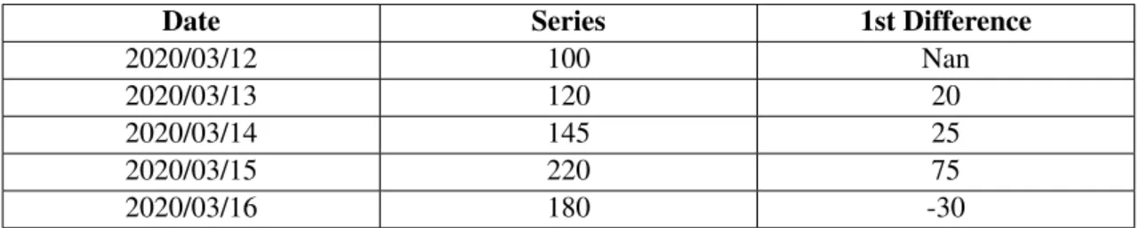
Table 2.1: Example of first order differencing.

Date Series 1st Difference

2020/03/12 100 Nan

2020/03/13 120 20

2020/03/14 145 25

2020/03/15 220 75

2020/03/16 180 -30

2.1.1 Naïve and classical forecasting methods

Naïve models applied to forecasting consist of simpler alternatives. Albeit its simplicity they are still used, specially when data is very constant and stable, due to their low complexity. On the other hand, there is evidence that they can be optimal when data follow a random walk [30]. There are several naïve methods, as seasonal naïve, predicting the exact value as any other previous period and drift method which allows the forecasts to increase or decrease over time based on a drift calculated as the average change observed in previous real observations [30].

Classical forecasting techniques present a wide range of algorithms from simple methods, such as Simple Moving Average (SMA), that calculates the forecasting value based on an average of a defined number of previous observations, to more complex ones. SMA, whence many other methods evolve, is connoted as the base of a high quantity of methods to analyze time series [30]. SMA does not adapt quickly to changes in trends and requires the storage of big quantities of data [18]. Exponential Smoothing appears as an improvement of SMA, since it uses the same principle but gives greater weight to the most recent data points [18]. These methods are part of time series models, that also aggregates Autoregressive Integrated Moving Average (ARIMA) and its variations.

ARIMA is complementary to Exponential Smoothing models and aims to describe correlation in the data [30]. This algorithm is a form of regression analysis that gauges the strength of one dependent variable relative to other changing variables. It can be subdivided into three capabil-ities: Autoregression (AR), Integrated (I) and Moving Average (MA). This method rests on the assumption that the time series is stationary [5]. Time series can be stationary or it can achieve such status through differencing. The first-order differenced data takes the increases between timesteps in the original data. Subsequent higher order differencing (order N) applies the same principle to order N-1 differenced data. The original time series is obtained through integration. Differencing concept is illustrated in Table2.1. In Figure2.1there are two graphics representing a non stationary time series2.1aand a stationary one2.1b.

Exponential Smoothing methods are weighted averages of previous observations whose weights decrease exponentially as the observations get older. Holt Winter’s Models is presented as an algorithm integrating exponential smoothing methods, with two variations Additive and Multi-plicative. This method is also known as triple exponential smoothing due the three smoothing equations that describes it for level, trend and seasonality [30] and the three correspondent pa-rameters α , β and γ. Trend is the component that changes over time and does not repeat itself

2.1 Forecasting techniques 7

(a) Non stationary time series due to visible positive

trend. (b) Stationary time series.

Figure 2.1: Example of time series non stationary and stationary.

and seasonality is the tendency of time series data to have behavior that repeats over time [35]. Summarizing the differences between additive and multiplicative approaches, the additive model is used when seasonality is expressed with the sum of a value, while multiplicative is used when seasonality corresponds to an increase of a percentage.

The previously referred methods have been widely used in different contexts. It is possible to find a considerable number of works that test different algorithms applied to a wide range of areas. For example, in electricity demand preview several works have been published over the past decades. Javedani et al. [33] compared five classical methods, Naïve, Holt Winter’s Multiplicative and Additive methods, Decomposition both Addictive and Multiplicative and regression, ARIMA. This study used 66 quarterly data observations with an outlier and was divided into two groups. The first group was used to train the model and the second group to test and compare the results. Concluding, the authors realized that Holt Winter’s Multiplicative method obtains more accurate forecasts than the others.

Da Veiga et al. [20] conducted a study comparing ARIMA and Holt Winter’s Multiplicative Model, within the scope of food retail demand forecasting. This research counted with 8 years of data of the specific type of products with a short life cycle. The results show that Holt Winter’s Multiplicative method has more accuracy when the predictions horizon does not extend the sea-sonal cycle of the time series. ARIMA model has many assumptions as persistence of historical patterns that, when true, guides to increased accuracy and very good results.

A survey on modeling and forecasting call center arrivals provides some insights on the most used techniques, in practice. Although the evolution of research and development of more sophis-ticated forecasting methods applied to this domain, the results are not being implemented in real contexts [32]. In this domain, ARIMA was presented as one of the earliest efforts to predict it. With the evolution in standard techniques, this algorithm continued being applied with some im-provements such as the inclusion of exogenous variables. Contrasting, the same author indicates that a considerable number of call centers were using simple methods implemented in Excel, at

8 Literature Review

the moment of the study.

A recent study [51] on sales forecasting aimed at presenting a new algorithm selection, com-pared several forecasting techniques. Focusing on the methods without external factors, 15 ods, ranging from classical to machine learning, where compared. Vouching for classical meth-ods, researchers concluded that ARIMA with additional seasonal components and Exponential Smoothing outperformed the rest.

A more recent approach to address time series forecasting is Prophet, proposed by Facebook, to handle common features of business time series which are characterized by trend, multiple seasonality, and holidays [49]. Prophet is considered interesting to process daily periodicity data with large outliers and shifts in trends with the advantage of modeling several seasonality peri-ods simultaneously [54]. Papacharalampous et al. [42] compared a set of methods to predict hydrometeorological time series, and concluded that Prophet is a competitive method in that do-main, despite nothing similar was previously applied. Zhao et al[54] applied Prophet to predict the concentration of fine particulate matter and considered that the algorithm reduces the impacts of problems such as data missing and unexpected outliers. Analyzing the trends of energy consump-tion on buildings Prophet was compared with ARIMA model Gong et al. [27] concluded Prophet presents lower MAPE then ARIMA. Another study on retail sales forecasting used Prophet to pre-dict the sales of 200 products of the 400 in their catalog. The results obtained with lower MAPE in most of the products for monthly and quarterly predictions denote satisfactory results, also, on this area [55]. Although it is a recently available solution, its implementations and results, denote the potential to be applied to business time series, considering the lower needs of preprocessing and the ability to deal with multi-temporal patterns and trends.

From the main categories of forecasting problems which are highly documented in the re-viewed literature, ARIMA models are presented as one that can achieve good performance, in many situations, being interpretable and with low complexity. Simple Exponential Smoothing and, its variations, also figure in the classical algorithms with the highest performance. Simple Exponential Smoothing is suggested also to Intermittent demand, described in section2.2, along with Croston’s method [46]. These two methods can be compared once they are indicated to the same target. Prophet is presented as an alternative state-of-art with advantages in time series data with strong seasonal effects and several seasons of historical data.

2.1.2 Machine learning applied to forecasting

Machine Learning (ML) can be defined as the ability a computer has to learn from data, and then apply the results of that learning to new information without being explicitly programmed to it. The machine receives a set of inputs and, then, learns from experience [29]. With high access to big quantities of data, and machine learning improving and getting good results, there is growing interest in exploring these algorithms [17]. Due to the capacity of ML, the forecasting domain also can benefit from its usage.

There are several comparisons, in literature, between different algorithms available. These algorithms include, but are not limited to, Neural Networks (NN), Recurrent Neural Networks

2.1 Forecasting techniques 9

(RNN), Random Forests, Gradient Boosting Machine (GBM) and Generalized Linear Model (GLM), briefly described in the following list:

• Neural Networks are an approach inspired by how a brain and nerve system works captur-ing the idea that the system can be nonlinear and non-parametric. It has capabilities to deal with more complex and non-linear relationships.

• Recurrent Neural Networks can be described as learning machines that recursively com-pute new states by applying transfer functions to previous states and inputs.

• Random Forest algorithm consists of a set of decision trees which are structured regressors, created during the training and whose output is, for regression methods, the mean of them. Breiman [16] considers random forests effective in prediction with the advantage of do not overfit.

• Gradient Boosting Machine (GBM) is a tree-based method that intends to improve pre-diction accuracy by combining the responses of previously executed algorithms [40] and is used in the context of ensemble techniques as detailed in the next subsection. Inside the context of ML, GBM produces interpretable results, once provides each predictor weight on the final model [53].

Some authors conducted studies comparing different algorithms in different contexts, con-tributing to an overview of the performance of each one of the methods. Alon [7] compares Neural Networks and traditional methods with the former outperforming the latter in three of the four cases evaluated in the context of aggregate retail sales.

In the context of food sales predictions, Tsoumakas [50] describes some machine learning techniques. This area cares of special attention when forecasting once the products have a short shelf-life and each error can lead to losses, when under or over predicting. Although the author specifies that the machine learning technique is more powerful and more flexible, when imple-menting in real business contexts the increase of lead times due to the complexity of the algo-rithms, is not always reasonable.

Forecasting inside a business context cares of an explanation of obtained results and statistics and evaluation metrics may not clarify what is happening to obtain the presented results. Ease of interpretation is considered one of the more important characteristics when selecting a forecasting technique [52]. Moreover, complex techniques are considered a challenge in terms of implemen-tation due to the users’ understandability and openness to them [6]. Also, NN has been criticized for the lack of interpretability, as Lasek [37] argued.

2.1.3 Ensemble techniques

The aforementioned algorithms produce forecasts that can be combined in order to obtain more accurate predictions. There are two types of strategies to address this technique, competitive and cooperative [44]. Competitive ensemble forecasting aims to combine the values from different

10 Literature Review

models, models constructed with different initial conditions or different parameters. The final pre-dictions are given by a combination of the prepre-dictions of the selected methods. This strategy gains with diversity though similar inputs lead to a combination also similar. Cooperative ensemble is obtained by aggregate the different predictions obtained by different models when forecasting sub-tasks of the all prediction objective. There are different strategies to answer the dataset division [44].

Focusing on competitive ensembles, there are several types of ensembles varying from linear combination to tree-based methods. A simple ensemble approach is to take a set of predictions and combine them equally weighted, resulting in a forecasting that is the average of the others. On the other side, GBM calculates the best combination of the predictors, within certain restrictions such as time and number of trees generated.

2.1.4 Algorithm selection

There are several forecasting methods, each one with its specific characteristics, and it is not possible to select the "best" one [22]. One method can produce valuable results under specific criteria and present failures under others.

When it comes to selecting a forecasting method the decision is rather intricate. In [8], Arm-strong introduces six different ways of selecting the forecasting algorithm to use, covering criteria that range from qualitative to statistical-based ones. First, the convenience by choosing a model the forecaster is used to work with, for example. This strategy might be useful when it is important to have a fast solution or there is not a significant impact induced by forecasting errors. Second, the Market Popularity which consists of select a method based on what is being used by others. This strategy can be based on the assumption that if a specific method is being largely applied it may de-rive from others’ research and experience which is also, a risky approach. Structured Judgement consists of developing a set of explicit criteria and based on this, compare the different meth-ods. From a previous study inquiring researchers, educators, practitioners, and decision-makers the top-rated criteria used when selecting a forecasting method, accuracy was on the top for all [52]. Statistical Criteria strategy is used when comparing quantitative methods and is based on statistics and due to its nature, based on a restricted selection, it can lead to misleading important information. Relative Track records consists of comparing the performance of different methods and is a good choice when the predictions have a high impact and, consequently, high errors too. The author considers the last approach useful and reliable but recognizes it imposes higher lead times and costs.

There are more complex approaches to select the correct forecasting method, such as develop a meta-learner that is able to learn from a set of time series the features that characterize each time series, and learn the appropriate forecasting model for each one of them, based on the lowest forecast error [36]. Although this approach leads to a better selection model on the tests developed, comparing four exponential smoothing models, it needs the development of the meta-learner and a wide range of methods is going to increase complexity.

2.2 Diagnosis and classification 11

Summarizing, model selection is a complex task and can be executed in different ways. From a statistical and data-driven point of view, the Relative Track records can be an accurate choice if the complexity of the tests and the time can be reduced.

2.1.5 Hierarchical structure

Although the algorithm selection is a very important process, under business conditions there is another category with high impact: data hierarchy. This concept exists on data that can be aggregated into different levels being an approach capable of integrating domain knowledge [21]. Under the domain of retail sales forecasting, the data can be easily aggregated into different levels. For example, the bottom level corresponds to each product (e.g milk, cheese), that can be aggregated into their category (e.g dairy products), which can be combined with other categories. This is a common practice in retailers once there are effects derived from small changes in prices, for example, whose impact on total revenue, at a top-level, is more easily captured than on-demand [25].

It is possible to have in the same dataset two types of hierarchies, for example, product, as the previous example, and geographic location of the stores that sell the products. The existence of two or more types of hierarchies that can be combined to produce different levels of aggregation leads to grouped time series [30].

There are three different approaches to obtain forecasts when predicting with different levels of aggregation:

• Bottom-up approach generates forecasts for each time series at the bottom-level and then sum them to obtain the predictions for all the structure levels.

• Top-down approach generates forecasts to the top level, first, and then disaggregates until reaches the lower level in the structure.

• Middle-out approach starts by selecting a middle level to generate forecasts. Then, com-bines both approaches, bottom-up to meet the higher levels and top-down to disaggregate downwards.

2.2

Diagnosis and classification

When conducting forecasting analysis there are several steps that can be performed before apply-ing forecastapply-ing methods. The data preprocessapply-ing can give important insights and lead to better forecasts. It can vary from highlight interesting relationships between data, detect trends, and identify and omitting outliers [10]. Classifications are important to understand the overall dataset composition and mostly used to obtain information relevant for inventory control [14].

Classifications

Items classification plays an important role in several industries. It can help to understand the inventory items better through different possibilities of classification. Through them, it is possible

12 Literature Review

to obtain valuable information on the items, represented by time series, forecastability and to infer important information to supply chain management, for example. The main classifications are:

ABC: rank items according to the periodic turnover. They can be classified by two approaches - quantity or sales. The principle consists in sorting the items descending by one of the categories, quantity or sales, and the cumulative sum is calculated. Then, to attribute the classification of A, B, or C to each item the distribution is usually based on ideal Pareto principle (80:20) [45]. This leads to less but more valuable A-items and numerous C items with low impact on sold quantity or sales amount.

XYZ: evaluates each item variations in consumption or demand. To obtain it the coefficient of variation is calculated and sorted by it. Then, it calculated the cumulative sum of all the items and, three groups are created based on defined boundaries [4]. Usually, the items are equally divided so each category has 33% of the items. Analyzing, X-items are constant, while Y-items have strong fluctuations in consumption which can be associated with trend or seasonal conditions and Z-items are irregular.

ABC analysis presents a rough classification due to the reduced number of categories [1]. Its quality is improved when ABC is combined with XYZ, constituting a matrix of nine possible classifications. With it, the classification is now based on values and demand frequency. Describ-ing the mappDescrib-ing between these two types of classifications, an AX item has high sales value and constant demand while a CZ has low sales value and sporadic demand.

Smooth, Erratic, Intermittent, and Lumpy classification is based on two values: average inter-demand interval (ADI) and squared coefficient variation (CV2) [48] and appears as an alter-native to classify items forecastability. Each category is defined as follows:

• Smooth: ADI < 1.32 and (CV2) < 0.49 • Erratic: ADI < 1.32 and (CV2) > 0.49 • Intemittent: ADI > 1.32 and (CV2) < 0.49 • Lumpy: ADI > 1.32 and (CV2) > 0.49

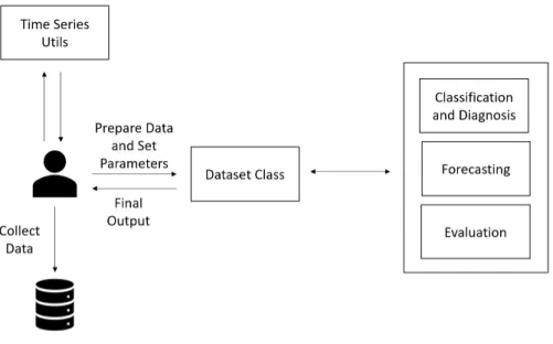
The graphical aspect of a time series of each category is presented in Figure2.2, where Vari-ability in demand quantity corresponds to (CV2) and Variability in demand timing relates to ADI. Smooth items are the ones where forecasting accuracy is expected to be better, while lumpy items refer to the opposite.

All the classifications can be used in data analysis before forecasting, but also to evaluate the performance in each category after it or even to create different models for each category, as suggested in4.

Outliers

Outliers can be defined as data points with a high deviation from the remaining ones, denoting an abnormal behavior. Outliers can be present in the x-axis and y-axis although, in time series analysis the ones in the y-axis are the most critical.

2.3 Evaluation metrics 13

Figure 2.2: Graphical representation of demand in each category of SEIL classification, [26].

Time series data usually has values considered outliers that can affect the different steps of a forecasting analysis like model identification, estimation, and forecasting [47]. The presence of outliers can lead to worst forecasting accuracy [34].

The treatment of outliers can be to remove these data points or replace them with a defined value that can be based on some time series metric.

2.3

Evaluation metrics

Metrics are necessary to compare different models in order to identify which of them produce better forecasts. The metrics selected must give a clear overview of the accuracy of the results.

The process of comparing algorithms starts with a common principle: every model uses part of the data available as a training set, also called in-sample, while the reminiscent data is used to test the model [30]. While the first set is used to fit the model, the second sample uses the previously defined model to forecast and, then, it is possible to compare the resulting set of forecasted values with observed values.

Evaluation metrics can be divided into three types scale-dependent errors, percentage errors and scaled errors [30]. In the first type, the errors are measured on the same scale as the data which means that cannot be compared with other series with different units. Percentage errors, due to its nature, are unit-free and allows comparison between datasets with different units. The last type is an alternative to compare different datasets based on percentage errors. Each type contains different metrics that can be relevant to address different forecasting problems. Amidst those metrics are:

• Mean Absolute Error, MAE, which is used when forecast models were applied to a single time series or several, using the same units [30]. As it is not a percentage, its interpretation

14 Literature Review

depends on the specific cases.

• Mean Squared Error, MSE is the average of the squared error.

• Root Mean Squared Error, RMSE, corresponds to the standard deviation of prediction errors.

• Mean Absolute Percentage Error, MAPE, that represents errors as a percentage, for each value forecast.

• Symmetric Mean Absolute Percentage Error, SMAPE, is an adaptation of MAPE aiming to equally weight under and over forecasts

• Mean Percentage Error, Bias, represents a historical average error, to understand if pre-dicted values are, on average, over or under forecasted.

• Mean Absolute Scaled Error, MASE, consists of scaling error based on the training data MAE from the naïve method.

• Theils’ U2 Statistic is a relative measure that addresses the forecasted values against the result of predict using a naïve strategy. It intends to measure the series forecastability. This statistic penalizes more large errors.

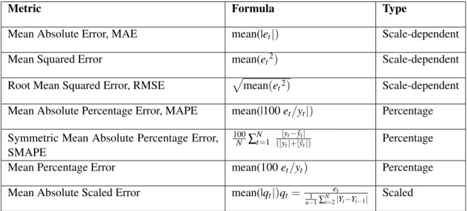
In table2.2formulas to calculate error and scaled error and previous described evaluation metrics are presented:

Table 2.2: Evaluation Metrics

Metric Formula Type

Mean Absolute Error, MAE mean(|et|) Scale-dependent

Mean Squared Error mean(et2) Scale-dependent

Root Mean Squared Error, RMSE pmean(et2) Scale-dependent

Mean Absolute Percentage Error, MAPE mean(|100 et/yt|) Percentage

Symmetric Mean Absolute Percentage Error, SMAPE 100 N ∑ N t=1 |yt− ˆyt|

(|yt|+| ˆyt|) Percentage

Mean Percentage Error mean(100 et/yt) Percentage

Mean Absolute Scaled Error mean(|qt|)qt= 1 et

n−1∑Ni=2|Yi−Yi−1| Scaled

In the formulas in Table2.2, the following symbols are:

• e: difference between real value, observed, and forecast value; • y: forecast value;

2.4 Technologies 15

• N: total number of forecast values.

These evaluation metrics differ and have advantages in different circumstances and are going to be implemented to calculate forecast accuracy.

Percentage errors, such as MAPE, are scale independent and, for that, can compare the per-formance of different data sets. Although this advantage, it is not performing so well once exist a predicted null value [31]. Positive errors have a higher penalty than negative errors, using MAPE. Afterward, MAPE is still widely used and preferred, when data has higher positive values, for its simplicity.

Once MAPE weights more over forecasted values, SMAPE is created trying to equal-weight forecasting errors. Although, Hyndman et al. [31] claim that this approach is not correct since it can be undetermined with a relatively common case: when predicted value is 0 and real value is 0, this metric is undertermined.

Hyndman and Koehler compare several accuracy measures and explains the pros and cons of them and also suggested a new measure, MASE. It is suggested when there are different scales and data points negative or close to null values. MASE analysis is, also, quite simple: when is higher than one, it concludes that, on average, naïve method performs well than method under analysis.

When comparing different time series there is a reduced set of evaluation metrics to help to compare the performance of algorithms between them. These methods are MASE and Theil’s U2 which intend to measure the time series forecastability. The main difference between them is that MASE is robust when there are actual or predicted values 0 while Theil’s U2 is undetermined when the naïve forecasts have a 0 value.

Evaluation metrics are crucial to lead to a complete and informed analysis addressing the quality of the forecasts. Each one of them can be useful under the restrictions and conditions, so it is important to have a wide range of them.

2.4

Technologies

Data-driven solutions are developed using large quantities of data collected through various meth-ods. Its storage is important to ensure data is accessible and fully integrated [24]. Data can be stored into Data Warehouses which can aggregate data from multiple sources. When comparing Amazon Redshift with Azure SQL Data Warehouse, two cloud data warehousing solutions avail-able, Ferreira [24] concludes that Amazon Redshift is easy to configure and setup but is more expensive when there is a necessity to scale data. Otherwise, the second solution computes and storage units are separated which makes it cheaper to increase only one of the components. On the other hand, it has an initial setup that takes longer.

There are available different programming languages and this number continues increasing. According to the IEEE Spectrum ranking of programming languages popularity, Python is leading since 2017. This popularity can be due to many specialized libraries of artificial intelligence [3]. Stack Overflow field a survey, every year, about different topics related to code. From the

16 Literature Review

2019 survey, Python is considered the fastest-growing major programming language and second preferred language [2].

Python aggregates libraries applied to forecasting and to data analysis that is efficient and effective. When compared to R, another language that has an extensive catalog of libraries applied to data science and forecast, Python is more general-purpose and more practical [29]. Python also has an extensive and active community developing content that can, drastically, decrease development lead times.

Concluding, Python is more indicated to deployment while R is more indicated to the imple-mentation of forecasting algorithms.

2.5

Exogenous variables in forecasts

Exogenous variables can add extra information to the time series that can improve forecast accu-racy. Their nature can be internal such as promotional information and last periods sales and also external for example macroeconomic factors or weather, supposing a sales forecasting problem.

VanCalster et al.[51] evaluate the value added by external variables comparing different mod-els with and without them. It is recognized that external variables increase explanation but also leads to higher maintainability costs. The execution of the different models indicates Seasonal Au-toregressive Integrated Moving Average with exogenous variables (SARIMAX) as the third best when comparing all models tested and the best forecasting method with external factors, based on MAPE. This model is considered transparent due to the understandability allowing to obtain the different weights of the exogenous variables. SARIMAX is an extension of ARIMA to deal with seasonal effects and exogenous variables. It is defined by seven parameters, three to classify trend, as in ARIMA, and four to characterize seasonality.

Weather is an external factor that can be, also, used as an external regressor. It impacts the economy [11] and is considered as an uncontrollable external factor, multiple times. Although this impact exists, it is a challenge to quantify sales related to weather conditions [9]. Weather can also be addressed as weather risk and can be divided into catastrophic and non-catastrophic [12]. Catastrophic refers to weather conditions not normal, such as storms, hurricanes, and floods among others. Otherwise, non-catastrophic refers to rain, heat, and cold, typical changes, and weather conditions that occur quite frequently [43]. Bertrand and Parnaudeau studied the impact of abnormal weather and stated that if companies that are more exposed to be influenced by weather variability understand how they can mitigate this risk and losses related to abnormal weather, they would get improvements and be well prepared to face problems [15].

Adding variables that in the future are also predictions, as weather, which is not known but only forecasted into the future, cares of special attention. In the train sets the values must be, also the predictions and not the verified conditions, predicted with the same time window.

When selecting external variables it means, usually, to increase complexity. Although these models can outperform simple benchmarks there is not enough evidence that this is an excellent approach [25].

2.6 Summary 17

2.6

Summary

Concluding the literature review chapter, this section intends to present an overview of the afore-mentioned topics.

Along this section, the different forecast techniques and some of their field applications were described. From the naïve algorithms, the simpler methods that can either work as forecasting methods or a benchmark to address how well are other methods performing when compared with them. The classical forecasting techniques are explored and it is verified that they are still used and obtaining good results. This can be a consequence of their high interpretability, reduced complexity, and overall implementation and reduced execution times. This is a motivation to take these models into account when forecasting. Inside the domain of ML algorithms, the field results are relevant but when centering on real data and in a business context the increase of complexity, the challenge in creating a generalization applicable to different time series, and the loss of comprehension are barriers to their implementation. Ensemble techniques appear as an alternative to combine previous methods predictions which can happen in more traditional formats or using an ML algorithm, GBM, that can explain how the predictions are generated. With a high variety of methods, the algorithm selection is not an obvious choice and cares for statistical evaluation of accuracy metrics as well as some business expertise. An additional characteristic, hierarchical structure, can add business information due to the grouping of the different items being predicted.

Each forecasting process concerns of analysis before the implementation of algorithms. These analyses can be more general purpose or more specific as classifications to characterize the differ-ent time series contained in a single dataset.

The analysis of time series followed by an implementation of forecasting techniques cares of evaluation, in order to simplify the choice of the final algorithm. Evaluation Metrics are the main measure to compare different forecasting strategies. Each one has advantages and disadvantages so, due to the number of different methods that can be tested before selecting the more adequate, it is important to have a wide range of them.

As time series forecasting is a complex process, adding external information as predictors lead to accuracy improvements, which makes it crucial to extend forecasting algorithms to consider these factors. For example, weather forecasting is selected as one variable that could impact most demand and sales in the retail industry, as well as business related characteristics.

Considering that there is not a tool compiling several forecasting techniques allowing users to test and compare results at once having the hierarchical concept implemented automatically and exogenous variables support, the need for a tool combining several algorithms and allowing agile development of forecasting techniques, arises. It is also noted that the inclusion of an analysis of statistics for data preparation and classifications can add value to building a powerful tool to answer business forecasting needs.

Chapter 3

Problem Description

Forecasting constitutes a necessity for multiple industries in order to improve their processes in a wide range of areas. The ability to learn from past events, applying that findings in modeling the future is a great advantage to leverage business. Organizations need to be prepared to face the future under uncertainty with forecasting systems tailored to their business needs. The devel-opment of these systems needs expertise in the process of forecasting to: apply a set of different algorithms, evaluate them and after selecting the one best fitting their needs, control its behavior throughout the future [30].

The iterative process mentioned becomes more complex when it is not executed one time to predict an organization future, but multiple times by a consultancy company operating in the de-velopment of data-driven solutions to help clients make more informed and better decisions across different areas. This is the case of LTPlabs, whose projects have a high incidence of forecasting. These projects are present on a daily basis, where they can be the main goal of the project or just a step to meet a need in other domains. There is space for improvements on forecasting processes since there are several algorithms and processing techniques to address them, however, they are not combined into a single place in an accessible and standardized way.

This chapter aims at detailing the identified problem and needs. The first section encompasses a detailed description of the forecasting approach followed at LTPlabs, in section3.1. In section

3.2the application of the methodology is presented along with the problems verified using it. In the end, holistic description of the proposed approach to mitigate the issues is provided.

3.1

Current forecasting approach

The current forecasting methodology adopted at LTPlabs can be described as a long and complex process. The current approach, followed by a considerable part of the forecasters, is illustrated in Figure3.1. The Cross-Industry Standard Process for Data Mining, CRISP-DM, is the most used methodology to guide the development of data mining and exploratory projects. Although it was conceived in 1996, it gained popularity in the market around 2000. It is analyzed by Matinez-Plumed[39] twenty years later and is considered still appropriate for predictive processes.

20 Problem Description

Figure 3.1: The CRISP-DM process model of data mining, still applied to forecasting.

The initial step executed is Business Understanding. It consists of understanding the main goals of a project and, consequently, collecting the requirements from a business perspective. The accumulated expertise of those who are familiar with data and have business knowledge is important to help in defining the main objectives and focus of forecasts. The results of Business Understanding stage can change the direction of the forecasting strategy and approach. It is impor-tant that business needs and constraints are well defined at the beginning to allow a faster process. Though, the need to complete or exploit information from the business is an available option that can be followed once the evaluation of a model denote it.

The next stage, Data Understanding starts with the collection of data and continues with a set of procedures to allow a better comprehension of it. First, it is necessary to collect data that can be from different sources which leads to a need for standardization. The next procedures can be from different natures such as interpret all data metrics, as mean, maximum and minimum values, check size, and attributes or even analyzing it graphically plotting different characteristics. This phase is the most lingering, focusing on increase familiarization with the data.

The Data Preparation covers all the steps to create the final time series. At this moment it is necessary to select data, to collect additional data sources, which can be either external, such as weather variables, or internal, as to whether a product is under a promotional campaign or not. Moreover, it is during this phase that is usually identified and removed outliers and selected the aggregation levels.

The Modelling phase incorporates the selection of an algorithm to apply and its parameters, the preparation of the train and test sets, as well as selecting the time windows for each one of them, and there is space for its optimization, by choosing more adequate values. This phase is executed multiple times, being selected a different algorithm at each cycle.

3.2 Forecasting application 21

Evaluation stage is a deeper analysis of the previously selected algorithm results. It is the mo-ment to confirm the impact of the strategy, comparing with the defined forecasting goals. More-over, it gives insights on how to improve the model.

When the Evaluation is favorable, the Deployment occurs. It comprises the process of trans-forming the defined algorithm and the test created into the forecasting process of some entity.

The process described, constitutes a long journey, because it is an iterative process that needs high investment in understanding the problem from a business perspective, to analyze data and then to select different algorithms and test them. Each test of a new algorithm requires high effort, which can lead to a reduction of the algorithms tested under time constraints. There is not a suggested number of algorithms to test until selecting the one that is going to be deployed, so the user expertise can be the trigger to understand when the results are good enough. Lack of time can be another trigger to stop the iterative.

Modelling and evaluation stages are repetitive tasks. These two processes are strongly con-nected since every model tested cares of an evaluation that can be, statistically, based on several metrics as previously described in section2.3. Evaluation can also benefit from user expertise to critical extract information from them and to map it with the Business Understanding.

3.2

Forecasting application

The current framework followed to address forecasting projects works with projects highly cor-related with business, due to the strong correlation with it, aiming to clearly define the business context needs.

Under a consultancy context that creates forecasting models to support multiple areas, these processes lead to time invested in the implementation of algorithms and evaluation metrics for each new project. Those implementations are, in general, tailored to the specific data available which can have different formats and come from many different sources. Although, the algorithms selected can not be the same performing the final solution, the path to achieve it has a number of them coincident.

After each forecasting project, there is knowledge acquired by practitioners. It can provide insights on best practices, model selection for specific cases or conditions, and on the accuracy metrics interpretability, for example.

Each forecasting project can have a different team assigned and the final solution is dependent on them. The previous experiences, the research background, and even the programming skills influence the way that the final solution is going to be traced and carried out. The change of teams, also difficult the spread of feedback, best practices, and strategies followed in previous works.

With the previously referred methodology to address forecasting inside business, there is space to leverage this process as there are some inherent drawbacks:

Rework: In each project, there are several concepts implemented such as analysis, algorithms, and evaluation metrics that are common, independently from the context of the project.

22 Problem Description

Non Standardization: Due to the different teams constituted to solve each new project, the methods used in the implementation of each technique are not concise across the organization. When there is no standardization, each solution will tend to a reaction to the specific problem instead of an application of a deliberated structure common to the entire organization. Although the methodology implemented is the same, there are no guidelines on best practices and recom-mended approaches for each one of the phases to follow. One of the goals, with standardization, is to reduce costs and consequently improving competitiveness in the market.

High lead times: This is, first, a consequence of the previous two problems. There is a part of the process explained in the previous section, that have to be addressed individually to correctly define the main goals and the focus of the forecasting. However, the implementations of common processes already done can be reused to reduce the development times. Thus, it is possible, from a business perspective, to reduce inherent costs.

Analyzing the forecasting projects completed at LTPlabs, the duration of the four phases, executed iteratively, from Data Understanding to Evaluation is, on average seven working days. Throughout an internal survey, it was possible to conclude that there is a work being repeated, mostly due to difficulties in the interpretation of the previous implementations of algorithms and due to being completely focused on the specific data of the project.

The selection of the models to implement is mostly guided by three factors. First, using the previous expertise on similar projects and selecting the ones with the best performance, then, on time series characteristics, obtained by the application of different classification techniques. Lastly, it is taken into consideration if the models being implemented are similar in terms of implementation and requirements or are inside the same interface, to reduce development times.

The implementation of an algorithm is usually based on a library from a specific programming language that can contain a single algorithm or a set of algorithms linked in the same way. For example, when selecting a classical algorithm such as ARIMA, the user chooses a library with it and format the data to meet its requirements. Then, all the algorithms present in there can be used in a similar way, since there is consistency in data inputs in the most used libraries. However, if the user intends to experiment a model from a different interface, to address the problem with an ML strategy, for example, the initial data preparation has to be executed again to fulfill the requirements of the new library.

When focusing on the evaluation phase, it is agreed that standardization of this process can lead to a fast observation of the metrics without implementing them saving time to spend in the following steps of the project, when the accuracy is not the focus for the final solution.

3.3

Proposed approach

In this section, it is described the proposed approach to tackle the problems defined aiming to reduce high lead times and contribute to other related processes improvement.

It consists of the development of a framework capable of allowing users o have a solid base to produce forecasts, both for junior users, that can obtain an overview of the forecasting process

3.3 Proposed approach 23

with lower inputs, and expert users who can add their expertise to obtain more insights or to guide the forecasting process in their own way.

At the initial phase, it is necessary to collect the requirements allowing a better understanding of the needs and main features among the forecasters. Then, it is necessary to structure the frame-work base of implementation and to define the structure of the information to be incorporated. Entering the forecasting domain, the implementation of data analysis tools is needed as well as the evaluation metrics that are going to allow an overview of the behavior of the algorithms throughout the development. For that reason, the next step is implementing each algorithm and, in the end, extend the framework with additional features to support grouped forecasting and the inclusion of exogenous variables. These sequence of steps is detailed along the following section

When this project started, at LTPlabs, the two initial phases were already completed existing the basic structure and definition of the principal framework units.

Evaluating the performance of the framework proposed, it is tested in four case studies, being three of them real business problems, previously addressed there.

Chapter 4

Methodology

The current chapter aims at detailing the proposed approach to reduce forecasting development effort and ensure thorough testing while generating forecasts in time constraint environments. Section4.1 details the proposed approach. The high-level framework structure and information organization are explained along section4.2. The development starts along with the implementa-tion of the diagnostic and classificaimplementa-tions described in secimplementa-tion4.3and section 4.4. In section4.5

it is covered the inclusion of different evaluation metrics. Section4.6describes the process that ensues the integration of forecasting algorithms in a standardized way. In section4.7the frame-work is generalized to include exogenous predictors in an effort to yield more accurate forecasts of the target variable. The chapter concludes with remarks on hierarchical forecasting strategies, in section4.8. Across all the sections the implementation is described, along with the defined default behavior when some specific information is not defined by the user.

4.1

Proposed approach

The framework succinctly described in the last chapter intends to group the main forecasting tech-niques, a set of preprocessing tools and evaluation metrics into a high-level framework, mitigating the issues of the current forecasting approach.

The forecasting procedure is extensive, in most of the cases, since it covers plenty of steps until the effective output of a prediction. There is a need to prepare data, which can come from different sources and to analyze it in order to extract valuable information. These initial processes can be executed to reduce the number of human input mistakes, or due to machine incorrect out-puts or, even, errors. The initial effort to clean the data and to analyze it is one of the most difficult parts of the procedure. Although there are several packages incorporating forecasting techniques, there are no tools to completely address those steps, into the same packages. The proposed ap-proach to develop the high-level framework is illustrated in4.1, whose organization is created and projected to support the complete implementation of all functionalities that are going to support the forecasting procedure. The steps guiding the implementation are similar to the followed when

26 Methodology

Figure 4.1: Proposed development approach of the framework.

executing an end to end forecasting analysis, except that, during development, evaluation metrics are implemented before the algorithms, as explained in section4.5.

The first phase consists in gathering requirements in order to determine the main functionalities expected. During this step, the path to follow throughout the development became more clear.

On the next stage, phase 2, structure and information organization, the framework is tech-nically detailed using the previously collected requirements, turning them into a system-specific description. At this point, the main constraints are defined in order to allow a link to all the func-tions within the module. Thus, the development starts with the implementation of the common structures that underline all the development and are responsible for the framework orchestration. With the main workflow defined, a strong and well-defined base fast-tracks ensuing developments. With an emphasis on grasping the general behavior of time series, the next development steps, phase 3, focus on algorithmic and diagnosis tools’ implementations. Phase 4 is the implementa-tion of several evaluaimplementa-tion metrics, that are useful to characterize forecasts. From the results of the evaluation metrics, it is possible to compare different algorithms used and to choose the one which best fits the data. At this point, the Framework contains the structure to do the early-stage analysis and to evaluate forecasts. These implementations care for several tests and validations that occur in parallel with the development.

From phase 3 onwards, the development includes testing to ensure a high level of generaliza-tion of the solugeneraliza-tion that has been developed each stage.

The proposed approach addresses what is the expected development of a forecast analysis, however, the evaluation metrics are implemented before the models themselves. This is required to guarantee that during the integration of algorithms, detailed along section4.6, there are enough tools to evaluate if these implementations are producing the expected results.

4.2

Structure and information organization

To support all the functionalities with different goals, it is necessary to define a structure of the in-formation allowing seamless communication between all the framework components. This struc-ture must be able to let the user communicate with all its components with a reduced set of com-mands, keeping both, customization and simplicity.