A Work Project, presented as part of the requirements for the Award of a Master Degree in Finance from the NOVA – School of Business and Economics
Money Never Sleeps – Overnight Returns in Equity Markets
Rafael de Almeida Sequeira 1019
A Project carried out on the Master in Finance Program, under the supervision of: Professor Pedro Lameira
Abstract
The present research analyses overnight returns’ outperformance in relation to daytime returns. In a first stage, it will be assessed whether these returns are robust throughout time, markets and across different scopes of analysis (e.g. weekdays, months, states of the economy). In a second stage, several hypothesis will be empirically tested, in an attempt to understand what drives non-trading period returns (e.g. liquidity, market volatility). Even though several authors have analysed overnight returns and suggested several explanatory factors, there seems to be no consensus in the literature regarding its drivers.
1. Introduction
According to Fama (1965), an efficient market is one where ‘on the average, competition will cause the full effects of new information on intrinsic values to be reflected “instantaneously” in actual prices’. In the literature, the rationale behind this statement is commonly referred to as ‘efficient market hypothesis’, and it argues that new information tends to spread very quickly among market participants; as such, market prices will reflect these changes almost instantaneously.
While this theory gained popularity in the 1960s, in the following decades great attention has been devoted to the study of market anomalies – patterns in securities’ returns that were (to some degree) reliable, predictable and yielded higher than expected risk-adjusted returns. Examples of these anomalies include the return of small-capitalization stocks (Banz (1981), Roll (1983), and Rozeff and Kinney (1976)), short-term mean reversion in individual equities (Rosenberg, Reid and Lanstein (1985), Lehmann (1990) and Lo and MacKinlay (1990)), momentum-like strategies in equity markets (Jegadeesh (1990), Chan, Jegadeesh and Lakonishok (1996), and Jegadeesh and Titman (2001)) and several calendar-based anomalies, such as the Monday, January and turn-of-the-month effect (Lakonishok and Smidt (1988)).
Based on this rationale, the present research intends to study an anomaly associated with non-trading period returns, which tend to be substantially higher than its trading period counterparts. Although some authors have suggested possible reasons to explain this anomaly, there is no general agreement regarding its drivers, as overnight returns do not appear to be fully explained by known risk factors.
This research is organized as follows: section 2 covers the literature review on overnight returns; section 3 discusses the methodology; section 4 presents the empirical results and discusses whether these are in accordance with previous literature; section 5 presents the main conclusions; section 6 contains the references and section 7 encloses the appendixes.
2. Literature review
This paper will address a known phenomenon – the effect of non-trading periods, when compared to trading periods. While many researchers have traditionally focused on the analysis of daily returns (i.e. which tend to be measured by close-to-close returns), more recently, their attention has shifted towards studying the different dynamics of trading and non-trading periods, namely daytime and overnight returns. This topic was initially addressed by Fama (1965), French (1980), French and Roll (1993), who concluded that non-trading periods were more volatile than trading periods, in the US equity market. Amihud and Mendelson (1987) found that volatility is greater from open-to-open, when compared to close-to-close returns.
Hong and Wang (1995) addressed the average return of non-trading and trading periods, concluding that trading periods yielded higher average returns. In contrast, Keim and Stambaugh (1984) and Cliff et al. (2008), showed that overnight returns are significantly higher than daytime returns. Other authors such as Geman, Madan and Yor (2001), as well as Tompkins and Wiener (2008), focused on higher order moments and concluded that non-trading periods exhibit a higher degree of non-normality, when compared to trading periods’ returns. Based on this idea, Tompkins and Wiener (2008) argue that trading periods’ returns follow a diffusion process, while non-trading period returns tend to follow a jump process, as price may not behave continuously between the markets’ close, in a given day, and the open, in the following day.
Additionally, it is also relevant to consider the degree of exploitability associated to overnight returns. Barber and Odean (2001) reported that transaction costs (i.e. commissions and bid-ask spread) would make overnight trading strategies unprofitable. However, Lachance (2015) argued that transaction costs have decreased substantially in the past decade and that, therefore, overnight strategies may be profitable.
Concerning the drivers of overnight returns, various authors have tested and assessed the validity of different hypothesis. Cliff et al. (2008) tested whether factors such as size, liquidity, volatility and the correlation with the previous overnight or daytime returns affected current overnight returns. Berkman et al. (2012) studied the impact of retail attention and the degree of institutional ownership on the said returns. Lou et al. (2015) tested whether overnight returns may be explained by momentum and whether similar trading strategies would be profitable. Tompkins and Wiener (2008) studied the impact of regulatory changes, particularly the Basel I Accord (1998), in overnight returns, across different equity markets. Finally, Kelly and Clark (2011) suggested that traders tend to sell positions at the end of the day and re-establish their positions in the following morning.
Even though overnight returns were initially studied more than 30 years ago, there seems to be no consensus in the literature regarding the reason to why overnight returns are significantly higher than daytime returns, in some markets and in some time periods. The present research will assess the robustness of overnight returns in several equity markets, and consider which factors are likely to explain the puzzle associated to overnight returns’ clear outperformance over its daytime counterparts.
3. Methodology
The main dataset used in this research is composed of nine time-series of Exchange Traded Funds (ETFs, henceforth), which reflected the main equity indexes of the United States of America (US), Canada (CA), United Kingdom (UK), France (FR), Germany (DE), Switzerland (CH), Australia (AU), Japan (JP) and China (HK, which stands for Hong Kong). These time-series contained end-of-day data, and the period under analysis started on 31st December 2003 and ended on 31st August 20151.
The main advantage of using ETFs, rather than the respective indexes, is that indexes’ prices reflect the last transaction of each of the stocks which comprise the index, and not every stock will trade every minute. According to Ng and Masulis (1995), this is particularly an issue for opening prices ‘due to delayed openings for individual stocks’. When there is a delay, the closing price of the previous day is substituted for the unavailable opening price.
This fact has been broadly discussed in the literature and it is one of the main reasons why index prices are not commonly used for this type of analysis. Tompkins and Wiener (2008), for example, used futures data to study daytime and overnight returns. In the authors’ words ‘both the opening and closing futures prices represent actual transactions by market participants’. However, the present research was not based on futures’ prices, as that would require the use of intraday data2, which is not easily accessible (especially for nine different equity markets).
Concerning the methodology used in this research, a few remarks should be made: (i) most regression outputs contain robust3 standard errors and respective p-values, so as to potentially correct heteroskedasticity and serial correlation in the error terms; (ii) when discussing average returns, standard deviations and info Sharpe ratios, the metrics will be presented in annualized terms, considering that one year has, on average, 260 trading days, unless stated otherwise.
1 Appendix 1 contains a detailed description of the tickers of the said ETFs and the indexes these replicate. 2 Since index futures tend to have different trading hours than the respective indexes, end-of-day data would not
reflect futures’ price at the index open and closing, respectively.
4. Empirical Results
4.1. Robustness of overnight returns
The first evidence that overnight returns tend to provide higher returns than their daytime counterparts is shown in the figure below. For the nine countries under analysis, overnight returns always provided higher cumulative returns, from January 2004, until August 2015. In the least extreme case, the difference between cumulative returns is only 77.47 percentage points (US), while in the most extreme case this figure increases to 632.06 percentage points (Australia).
Figure 1 - Cumulative daytime and overnight returns, for the nine markets under analysis
Even though Figure 1 provides a clear image to the in-sample overperformance of overnight over daytime returns, it is important to test its robustness to assess whether this relation is spurious, and whether or not it would be expected to persist. As seen in appendix 2, for all analysed markets, the average return of the overnight period is always higher than its daytime counterpart, while the overnight average volatility is lower in all countries except Japan and Australia. Consequently, overnight returns yield higher info Sharpe ratios. These findings are consistent with Fama (1965), French (1980), French and Roll (1993), and Amihud and
Mendelson (1987) concerning overnight returns’ lower volatility and also with Keim and Stambaugh (1984) and Cliff et al. (2008) regarding the higher average return.
Regarding higher order moments, both types of returns tend to exhibit negative skewness; however, overnight returns tend to have a more negatively skewed distribution. The only exceptions are: Canada, where overnight returns are positively skewed, while daytime returns exhibit negative skewness; Switzerland, where overnight returns are slightly less skewed; and China, where skewness is positive for both types of returns, but overnight returns are more positively skewed. Concerning kurtosis, in every market, overnight returns exhibited fatter tails, when compared to its daytime counterparts. In some markets the increase was relatively small, while in other cases kurtosis in overnight returns was 2-6 times higher than in daytime returns. These findings are also in accordance with previous research (Geman, Madan and Yor (2001) and Tompkins and Wiener (2008)), in the sense that non-trading period returns exhibit a higher degree of non-normality when compared to trading period returns, which may be formally tested with Jarque-Bera’s test. Furthermore, in all markets except for Japan, the maximum drawdown of overnight returns was substantially lower. The average maximum drawdown across the nine equity markets was 124.84%, in the overnight period, and 34.27% in the daytime period. These findings support the hypothesis that maximum drawdown tends to be substantially smaller during non-trading periods, in most of the analysed markets.
In conclusion, standard deviations are not able to explain the significantly higher overnight returns. However, as overnight returns are not as normally distributed as daytime returns, the return difference could be explained by the jump risk that exists in overnight returns. However, Tompkins and Wiener (2008) argued that the jump risk was not being priced in a similar fashion across the five equity markets they analysed; therefore, it would appear unlikely that one market exhibits a low implied price for jump risk, while others have a significantly higher price. Thus, they concluded that jump risk would likely not be a relevant driver in overnight returns.
Furthermore, in order to assess whether overnight returns were significantly higher than their daytime counterparts, the following regression was employed4:
𝑟𝑡 = 𝛽0+ 𝛽1𝐷𝑡𝑁 ( 1 )
where 𝑟𝑡 is a vector where each daytime return is followed by the overnight return made in the following night and 𝐷𝑡𝑁 is a dummy variable that is equal to 1 if the return under consideration was made during the night, and 0 otherwise. As seen in appendix 3, at a 5% significance level, all markets except the US, Germany and Japan showed that overnight returns were significantly higher than daytime returns. However, as the p-values associated to Germany and Japan were both under 6%, the only ‘outlier’ was the US market, with a p-value of 17.4%. This last finding will be studied in detail in section 4.2.5.
Regarding calendar effects, both overnight and daytime return series were examined through the following scopes: day-of-the-week, month and year.
Starting with the day-of-the-week effect, in most markets negative daytime returns are concentrated at the beginning and at the end of the week. On Monday, all markets show large negative daytime returns (average return of -12.40%, across the nine markets), with the exception of Germany, which displays an average return of 2.71%; on Thursday, Japan is the only country with a positive daytime return (6.12%), while the average return of all countries is -12.90%. Finally, on Friday, the average daytime return is -7.68%, and Canada and China are the only markets with positive average returns. Focusing on the night period, most markets have, on average, positive returns in all weekdays, with the exception of Canada and Japan (i.e. each market has one weekday with a negative average return, respectively). Thus, the present dataset contains strong evidence that daytime returns exhibit what authors such as French (1980), Gibbons and Hess (1981) and Rogalski (1984) have identified as ‘Monday’ effect (i.e.
4 This procedure was similar to the one employed by Cliff et al. (2008). Moreover, the dependent variable was
tested a priori for unit-roots, through three specifications of the Augmented Dickey Fuller test, for lags from 1 to 20. In all specifications, the null hypothesis was rejected and the series were considered to be stationary, at a 5% significance level.
Mondays’ returns tend to be significantly lower than the remaining weekdays’ returns). On the other hand, overnight returns appear to be robust across weekdays.
Concerning different months, the ETFs’ daytime returns tend to perform poorly in January (i.e. all markets had average negative returns, and the average annualized return across all markets was -27.04%), May and June (i.e. where the average annualized return was -11.33% and -21.22%, respectively) and also in August and October (i.e. where the average annualized return was -10.34% and -6.10%, respectively). Considering overnight periods, the worst performing months were August (where Canada, UK, and Australia were the only markets with positive returns) and October (where Germany, France and Japan had negative returns); the average return across the analysed markets was -0.90% and 7.68% for these two months, respectively. This finding could be related with the fact that the most volatile months for both the daytime and overnight returns tend to be August through November, as measured by standard deviation. Nevertheless, this hypothesis will be further analysed in section 4.2.2. In conclusion, even in the worst performing months, overnight period still provide substantially higher returns when compared to trading periods.
Regarding returns-per-year, the worst performing years for daytime returns were clearly 2008 through 20115. In 2008, for instance, the lowest, highest and average daytime return were -70.82% (Australia), -6.55% (Japan) and -42.01%, respectively. Overnight returns, on the other hand, showed a maximum gain of 21.75% (AU), a maximum loss of -48.83% (JP) and the average return was -7.22%, in 2008. From 2009 through 2011, the pattern is quite similar, as there is at most one market out of nine where trading periods outperform non-trading periods. Therefore, on average, overnight returns appear to consistently outperform daytime returns in the time period under analysis. Moreover, by comparing the yearly info Sharpe ratios, it can be
5 Daytime returns had a poor performance from January until August of 2015. However, it would not be appropriate
to draw any conclusions from this period, as these could be biased (e.g. markets could have performed relatively well, in the remaining months of 2015).
concluded that overnight periods also tend to outperform daytime periods. In the least extreme case (JP), daytime returns have higher info Sharpe ratios in 4 out of 12 years; while, on the most extreme case (AU), daytime returns never have higher info Sharpe ratios.
Additionally, it was also assessed how overnight and daytime returns performed in different states of the economy6. In economic expansions, non-trading periods clearly outperform trading periods. The discrepancy between average returns is smallest in the US market (i.e. 7.12 percentage points, in annualized terms) and it is largest in the Australian market (i.e. 55.67 percentage points, in annualized terms). In economic recessions, 6 out of the 7 analysed markets7 exhibited average overnight returns that were larger than daytime returns. The only exception was Japan, where overnight periods yielded returns that were 1.37 percentage points lower than the daytime periods. Also, while the seven markets under analysis all had negative average daytime returns, four had positive overnight returns. In conclusion, in both states of the economy, overnight returns appear to outperform its daytime counterparts.
Finally, the last test for robustness was to split overnight returns into: (i) regular nights, (ii) regular weekends, (iii) regular holidays, and (iv) long weekends (i.e. when there is a holiday on a Monday and/or Friday)8. In regular nights, all nine markets exhibited positive average returns; in regular weekends, the French market was the only one with negative average returns (-0.87%, in annualized terms). Regarding regular holidays and long weekends, most markets display considerably high annualized average returns (with the exception of the UK, with a return of -11.16% in regular holidays), as well as high info Sharpe ratios. However, these last two categories likely suffered from small sample bias, as most markets had under 100 observations. On average, whether the market is closed just for a regular night, for a regular or long weekend, or for a holiday, the average overnight return tends to be positive and, in some instances,
6 Economic expansions and recessions were defined through the Economic Cycle Research Institute (ECRI)
database.
7 Australia and China (Hong Kong) were never considered to be in economic recession, in this timespan 8 The different categories for overnight returns were the same as in Tsiakas (2008).
particularly high. Furthermore, there appears to be no clear pattern between the length of the closing period and the magnitude of overnight returns – across the nine markets under analysis, there is no clear signs of under or overperformance of long disruptions (e.g. regular and long weekends) over short ones (e.g. regular nights and holidays). In summary, overnight returns are also robust to different types of market ‘disruptions’.
4.2. Hypothesis testing
After establishing that overnight returns are substantially larger than daytime returns, across different scopes of analysis, it is relevant to try to explain its drivers and whether or not they are expected to persist through time.
4.2.1. Liquidity
According to previous research (Pastor and Stambaugh (2001), Amihud (2002) and Cliff et al. (2008)), returns should be negatively related with liquidity metrics. When liquidity decreases in a given market, implicit trading costs (e.g. bid-ask spread) tend to increase. Amihud and Mendelson (1986), for example, have shown that small sized stocks have larger bid-ask spreads and that their prices are more sensitive to order flows. Riedel and Wagner (2015) also argue that overnight returns’ fat-tailedness is explained by the ‘lack of market functionality and liquidity’, which, in turn, causes the price jump at the market open.
In order to assess the relevance of liquidity in overnight returns, several metrics were considered9: (i) dollar volume, (ii) turnover rate, (iii) Hui-Hubel Liquidity Ratio (LHH, henceforth), (iv) Market-Efficiency Coefficient (MEC, henceforth), which was computed for the daytime and for the overnight returns, and (v) Amihud’s illiquidity measure. These liquidity measures were computed based on Bloomberg’s price and volume data10.
9 The bid-ask spread (both in dollars and in percentage terms) was also computed. However, according to
Bloomberg data, the bid-ask spread was negative for the majority of the ETFs under analysis, quite a few times along the time-series. Therefore, due to the lack of reliability of bid and ask prices, the bid-ask spread was not considered as explanatory variable to overnight returns.
10 The computation of the liquidity metrics was based on the formulas described by Sarr and Lybek (2002) and
According to Sarr and Lybek (2002), turnover is a simple measure that relates trading volume with the outstanding volume of the asset under analysis. Consequently, the turnover rate will indicate how many times the outstanding volume is traded. Also, according to these authors, the LHH Ratio attempts to relate volume to its impact on price. The lower the value of LHH, the higher the liquidity in that market. However, one of the criticisms of LHH is that when new information reaches the market, prices may suffer large upward or downward movements; thus, price movements are not directly related with the assets’ liquidity.
The MEC, on the other hand, considers that given a permanent price change (e.g. earnings information reaches the market), the transitory changes in price should be as small as possible, in highly liquid markets. Thus, this ratio should be close to (but slightly smaller than) 1, in resilient markets, and it should be lower than 1, in illiquid markets. Finally, Amihud’s illiquidity metric measures illiquidity as the average ratio between the daily absolute return to volume, on a particular day. The higher the measure, the more illiquid is the asset under consideration. Several authors, such as Amihud (2002), Chordia, Huh, and Subrahmanyam (2009), have shown that there is a positive relation between stock returns and this illiquidity measure, which should be related with the liquidity premium.
After building these metrics, the overnight returns of the nine markets under analysis were regressed against each metric. The results, however, do not show a clear pattern as to which metric better represents the theoretical negative relation between liquidity and assets’ returns.
At a 10% significance level, there are no significant relations between overnight returns and any of the previously described liquidity measures for the United States, United Kingdom, Germany and Switzerland. In Canada, Amihud’s illiquidity measure appears to be negatively related with overnight returns at a 10% significance level, which would imply a positive relation between returns and liquidity. In Australia, Japan and Hong Kong, however, the coefficient
Augmented Dickey Fuller test, for lags from 1 to 20. In the vast majority specifications, the null hypothesis was rejected and the series were considered to be stationary, at a 5% significance level.
associated to Amihud’s metric is positive and significant, at a 6% significance level. On the other hand, MEC was shown to be significant for three different markets: in France, an increase in MEC (computed with daytime returns) would lead to a decrease in overnight returns; while in Australia and Japan, it would lead to an increase in overnight returns. Since the average value for MEC is 0.379 (FR), 0.395 (AU) and 0.386 (JP), it is expected that overnight returns and MEC would have a negative relation (i.e. since an increase in MEC would make this measure closer to one, which would indicate a more liquid market, on average, ceteris paribus). Finally, Hong Kong’s market also shows a significantly positive relation between overnight returns and turnover ratio, which does not support the theoretical hypothesis.
In conclusion, given the mixed results presented in this section, it appears that overnight returns are not constrained to low liquidity in financial markets. These results are in accordance with Cliff et al. (2008), who argued that liquidity was not a significant factor behind individual stocks’ spread between overnight and daytime returns, in a robust manner.
4.2.2. Market volatility
As seen in section 4.1, overnight periods exhibited lower returns during the months of August through November, which coincided with the months of higher volatility both in overnight and daytime returns. In this section, it will be tested whether there is a relation between the overnight returns and volatility. In order to compute a variable which represents market volatility, a procedure similar to the one used by Longstaff (1995) and Cliff et al. (2008) was followed. As such, volatility was proxied by the standard deviation of close-to-close returns over the prior calendar quarter.
When regressing the average overnight returns of a given quarter on the previous quarter’s standard deviation, all coefficients are insignificant at a 5% significance level. However, if the average overnight returns of the current quarter are regressed on the standard deviation of the same quarter’s returns, the estimated coefficients are highly significant and all of them are
negative. Therefore, the present dataset shows a negative relation between ‘quarterly’ market volatility and the average ‘quarterly’ overnight return, which is always statistical significant at a 1% significance level.
Since using quarterly data leads to a relatively small sample, it was also tested whether the standard deviation of the close-to-close returns in the previous 5, 10, 20, 40, 60 and 100 nights had any impact on the following night’s return, through a regression. However, at a 5% significance level, all volatility measures were non-significant for the analysed markets. The same experiment was repeated, based on standard deviations of overnight returns (i.e. instead of using standard deviations based on close-to-close returns). Nonetheless, the coefficients were also non-significant, at a 5% significance level.
Regarding previous research, Longstaff (1995) has shown that stock returns during periods of ‘non-marketability’ should be positively related to the firm’s standard deviation; therefore, higher standard deviations should lead to higher overnight returns. Cliff et al. (2008) also argues that stocks with higher standard deviations have higher overnight returns than stocks with low standard deviations, even though both types of stocks have ‘statistically significant positive returns’, in the authors’ words. Since both authors used individual equities in their researches, these results do not contradict theirs directly, in the sense that our standard deviation metric measures the overall volatility of each country’s stock market, and not the volatility of individual equity returns, which contains both idiosyncratic and systematic risk.
4.2.3. Higher order moments
As shown previously, overnight returns robustly yield higher info Sharpe ratios than daytime returns. However, since Sharpe ratios measure risk through standard deviations and considering that returns do not typically follow a normal distribution11, the impact of higher order moments on overnight returns should also be analysed.
11 Hull (1993) and Corrado and Su (1996, 1997) have used the non-normality of assets’ returns to explain the
For this purpose, the skewness and kurtosis of previous nights were individually regressed on current overnight returns, with lookback periods of 5, 10, 20, 40, 60 and 100 nights. Concerning skewness, our dataset suggests that in the short-term (i.e. for lookback periods of 10, 20, 40 and 60 nights), there is a negative relation between past overnight skewness and current overnight returns, for the majority of the analysed markets. Moreover, for a lookback period of 5 days, all coefficients are non-significant; while for a lookback period of 100 days, nearly half of the relations are non-significant and the remaining half exhibited a positive ‘skewness premium’.
In the literature, the work of Theodossiou and Savva (2015) presented two interesting findings: (i) individual US equities displayed a negative skewness risk premium, which appears to be in accordance with our results for short-term lookback periods; (ii) the risk-return relationship (measured by the average return and standard deviation) may yield conflicting results12, depending on the ‘extent of negative skewness’. Since it was shown that low volatility periods were associated with higher overnight returns in section 4.2.2, and given that the theoretical relation between risk and return should be positive, this empirical result may be related with the negative skewness found in the said returns.
Regarding the impact of kurtosis in overnight returns, our dataset does not exhibit a robust relation between these two variables. For a lookback period of 5 days, there is a significant negative relation for France and Switzerland and a positive one for Australia. For the remaining lookback periods, the only significant relations were a negative one for Switzerland and Japan, and a positive relation for Hong Kong. Since Theodossiou and Savva (2015) suggest that kurtosis risk premium should have the same sign as the skewness of the assets’ returns, our findings appear to be in accordance with their reasoning. The average skewness only appears
12 French et al. (1987) and Lundblad (2007) found a positive risk-return relation, while Glosten et al. (1993) found
a negative risk-return trade-off, and Campbell and Hentschel (1992) and Theodossiou and Lee (1995) found a non-significant relation between these variables.
to be robustly positive across lookback periods for Australia and Hong Kong. Hence, the negative relation between kurtosis and overnight returns found in France, Switzerland and Japan seem to be consistent with this idea, as well as the positive relation found in Hong Kong. Nevertheless, the non-robust relation between kurtosis and overnight returns appears to be in accordance with the work of Arewa and Ogbulu (2015), who found a significant relation between returns and skewness, but an insignificant one concerning kurtosis. Chang et al. (2013) argue that individual equities with high sensitivity to innovations (as measured by market implied kurtosis) tend to exhibit higher average returns. However, these authors also shown that their results lacked robustness regarding the pricing of kurtosis risk; even though they appeared to be robust regarding skewness risk.
In conclusion, our results are in accordance with the empirical impact of both skewness and kurtosis. Even though most of the previously mentioned studies used individual equities and were based on close-to-close returns, it appears that a similar reasoning may be applied to overnight returns. As a reference for future research, it could be interesting to assess the impact of intra-day skewness and the following overnight return.
4.2.4. Correlation in overnight returns
Ng and Masulis (1995) have studied the daytime and overnight return dynamics, as well as the correlation structure of both types of returns. They found a negative correlation between overnight returns and its past lags, particularly from lags 1 through 3. Moreover, these authors also found a positive correlation between overnight returns and the previous day’s return, as well as some negative correlations with other lagged daytime returns, for lags between 2 and 5. Additionally, Lo and MacKinlay (1990) argue that negative autocorrelations tend to be a common assumption among most overreaction theories (i.e. theories which state that investors tend to react in a disproportional manner to new information and after large price movements, a correction in the opposite direction is likely to occur).
Our dataset seems to exhibit a similar pattern to the one found by Ng and Masulis (1995). Across the nine markets under analysis, there is a clear pattern of negative autocorrelations in overnight returns, from lags 1 through 3, as well as in lag 5. Regarding correlations with past daytime returns, there appears to be a positive relation in lags 1 and 5, a mixed relation in lags 2 and 4, and a negative one in lag 3.
Moreover, auto-correlation and correlations with past daytime periods were also analysed on a year-by-year basis, as correlations tend to be time-varying13. Across the analysed markets, overnight autocorrelations (particularly for lags 1, 3 and 5) show a tendency to decrease (becoming more negative, in most cases) in periods of high volatility, such as 2008 and the following years. This pattern is also present in correlations with past daytime returns (more specifically in lags 1 and 2), where most correlations become negative for most markets, even though the average correlation in-sample is positive.
In conclusion, past daytime and overnight returns may provide some information regarding the signal and magnitude of future overnight returns. Even after taking into account that correlations may increase or decrease throughout time, there is a clear tendency for autocorrelations to be slightly negative, in the period under analysis. Particularly, the negative autocorrelations in overnight returns are in accordance with overreaction theories, as discussed by Lo and MacKinlay (1990).
4.2.5. Persistence of overnight returns (United States of America)
As previously mentioned, the US was the only country where overnight returns were not considered to be significantly higher than daytime returns. In order to understand whether non-trading periods are expected to yield superior average returns in the future, it is important to understand if this ‘anomaly’ ever existed in the US; and if so, why and when did it disappear.
13 Particularly, Ng and Masulis (1995) consider structural breaks throughout their analysis, in order to capture the
different dynamics of overnight and daytime returns and volatility, through the analysis of correlations structure and GJR-GARCH coefficients across sub-samples.
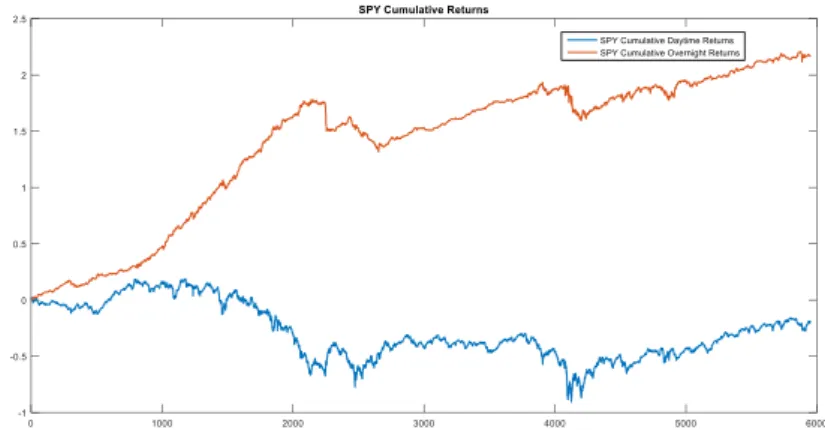
By extending the US sample, from 22nd January of 1993 until 31st August 2015, and plotting the cumulative returns (as in figure 2), it is clear that overnight returns yielded much higher returns than daytime periods, particularly from 1993 until 2001-200214. By performing the same regression as in equation (1) with this extended sample, the conclusion changes – overnight returns in the US are significantly higher than daytime returns, at a 2% significance level, as seen in appendix 21.
Figure 2 - Cumulative return of SPY US Equity, since 22nd January 1993 until 31st August 2015, split into daytime and overnight returns
Since this ETF was only introduced in 22nd January of 1993, in order to analyse in detail the ‘disappearance’ of overnight returns in the US, it was necessary to use a time-series that started at an earlier point in time. As such, end-of-day data from stocks that were constituents of the Dow Jones Industrial Average (DJIA, henceforth) was extracted from Bloomberg. In order to avoid survivorship bias, the composition of DJIA was extracted from Center for Research in Security Prices (CRSP), and its constituents from 1907 until 1979 were selected15. By examining the performance statistics of the 15 equities under analysis (appendix 24), the results are rather mixed. In fact, in only 6 cases, overnight periods yielded higher returns than daytime periods. Regarding the info Sharpe ratio, only 7 out of 15 stocks exhibited a higher
14 This small period contains the Internet run-up; however, since Cliff et al. (2008) analysed US equities from the
S&P 500, AMEX Inter@ctive Week Internet Index and also 14 different US ETFs, and overnight returns were robust across these different assets, the hypothesis that overnight returns over performance was solely or mostly caused by the Internet run-up will not be analysed in this research.
15 In appendix 22, there is a list of the dates of inclusion and, in some cases, exclusion from the DJIA. The
Bloomberg tickers and other relevant information is also presented in the said appendix. However, due to data unavailability by Bloomberg, only 15 out of the 18 DJIA constituents were considered in this analysis.
Sharpe during the night, versus the day. Concerning maximum drawdown, only 6 out of 15 stocks appear to have lower drawdowns overnight, rather than during the day. Still, it is important to stress that these 15 equities still represent a small fraction of the US equity market, and no conclusions can be drawn regarding the latter.
Nevertheless, given that the significance tests previously employed on SPY US Equity yielded two different conclusions for two different samples, it will be studied whether or not this ‘change’ in the behaviour of overnight returns may have been caused by a structural break. In econometric terms, Chow (1960) was the first author to suggest a structural break test, for the case where the break point was known. Andrews (1993) and Andrews and Ploberger (1994) suggested other test statistics, which do not rely on the specification of any particular point of change, such as supF, aveF and expF statistics.
Before elaborating any hypothesis to what might have caused the possible break in overnight returns dynamics, it is important to check whether the equities are likely to have suffered a structural break, through a parameter instability test16. Appendix 25 contains the main statistics associated to those tests. As seen by the SupF(1|0) statistic, at a 5% significance level, in 10 out of the 15 equities, the null hypothesis of ‘no structural break’ is rejected, against the alternative, which stands for the existence of one structural break. Regarding the remaining SupF statistics (where the alternative hypothesis is the existence of 2 to 5 structural breaks, respectively), the result is similar, in terms of rejecting the null hypothesis. Thus, for the majority of the equities under analysis, there is statistical evidence of the existence of at least one structural break.
Moreover, through the sequential process (Bai and Perron (1998)), it is possible to estimate the possible break dates and assess their significance. At a 1% significance level, there are 7
16 For the purpose of estimating possible structural breaks and evaluating their significance, a Matlab version of
Pierre Perron’s GAUSS code was used, which was developed by Yohei Yamamoto. This code was downloaded from Pierre Perron’s website, at the Boston University (http://people.bu.edu/perron/code.html). No changes were made to this Matlab code and therefore all credits go to the aforementioned authors.
different breaks, between the periods of 1992 and 2009. Appendix 27 represents the years where a statistically significant break was detected and the average year for the said breaks, for a significance level of 1%, 2.5%, 5% and 10%. The average break occurred between the years of 1998 and 2001, depending on the significance level considered. This result seems to be in accordance with the change in the behaviour of SPY US Equity (Figure 2), on average terms.
As it seems reasonable to assume the existence of a structural break in the US equity market, two hypothesis will be tested, regarding the reasons that could have caused the said break: (i) S&P 500 futures (SP, henceforth) started trading overnight, through GLOBEX, in 3rd January of 1994; (ii) the E-Mini S&P 500 futures17 (ES, henceforth) started trading in 9th September 1997, in both daytime and overnight periods. The rationale behind this hypothesis is fairly simple: as these future contracts started to trade overnight, investors could hedge their positions while the markets were closed. Therefore, investors could reduce exposure to the swings that might occur between market close and open and, since in the light of the risk-return theory, investors should not be rewarded for carrying risks that they could avoid, overnight returns should diminish in magnitude.
By conducting a Chow test for the first break point considered (3rd January of 1994), at a 5% significance level, 6 out of 15 equities show significant structural changes. Additionally, by performing the same test for the second break (9th September 1997), 8 out of 15 equities exhibit significant changes in behaviour. Then, in order to assess how the structural breaks influenced overnight returns, a similar procedure to the one used by Ng and Masulis (1995) was employed – a GJR-GARCH18 model was regressed before and after the structural break, for the two structural breaks under analysis19. The GJR specification was as follows:
17 An electronically traded futures contract that has one fifth of the size of standard S&P futures (SP).
18 GJR stands for Glosten-Jagannathan-Runkle, from the name of the authors who developed this model; and
GARCH stands for Generalized Autoregressive Conditional Heteroskedasticity.
19 Before regressing these models, each equity time-series was tested for ARCH effects, through an Engle test (see
Engle (1982)). As equities number 4, 8 and 15 exhibited no significant presence of ARCH effects, the volatility equation for these equities is not reported in appendix 29 through 32.
𝑟𝑡𝑁 = 𝛽0+ 𝛽1𝑟𝑡−1𝑁 + 𝛽2𝑟𝑡−1𝐷 + 𝑢𝑡 ( 2 )
𝜎𝑡2= 𝜔 + 𝛼𝜀𝑡−12 + 𝛽𝜎𝑡−12 + 𝛾𝜀𝑡−12 𝐼𝑡−1, 𝑤ℎ𝑒𝑟𝑒 𝐼𝑡−1= {
0, 𝑖𝑓 𝜀𝑡−1 > 0
1, 𝑖𝑓 𝜀𝑡−1 < 0
( 3 )
Considering the first break point, the intercept on the mean equation only appeared to decrease in 5 equities; in the remaining 10, this value increased. Moreover, for the majority of the equities, 𝛽̂1 decreased and 𝛽̂2 increased. In the variance equation, for most equities, 𝜔, 𝛼 and 𝛾 decreased, while 𝛽 increased. Regarding the second break point, the results were rather similar. Furthermore, it was also tested whether the differences in the intercept of the mean equation, before and after the break, were significant20. In the first break point, there were 6 statistically significant increases and 2 decreases. While in the second break point, these figures both changed to 5, respectively.
Finally, since the GJR’s mean equation included lags of the past daytime and overnight returns, another regression was built in order to assess if the average overnight return increased/decreased after the break: overnight returns were separately regressed on a constant, before and after the break,. Then, similarly to what was previously done in the GJR-GARCH specification, it was assessed whether the change in the intercept was significant. Considering the first break, 10 equities showed an increase in intercept, where 3 were significant at a 5% significance level; in the remaining 5 equities, only 1 of those decreases in intercept was significant. Regarding the second break, there were 9 intercept increases (2 of which were significant) and 6 decreases (1 of which was significant). In summary, both in the GJR-GARCH specification and in the latter regression, most equities’ average returns tends to increase after the structural break – which is against our initial hypothesis – even though most of those variations were not significant.
20 This was performed through a t-test, and it was assumed that both sub-samples were independent from each
As our findings suggest that the introduction of overnight futures, per se, did not lead to a decrease in overnight returns in the equities under analysis, a final hypothesis was tested: did the trading volume of equity futures impact equities’ overnight returns? The rationale of the initial hypothesis suggests that an increase in trading volume would lead to a decrease in overnight returns. Even though investors were able to hedge their trades overnight, trading volume in the SP and ES was relatively low in the years after these securities started to trade overnight (1994 and 1997, respectively). This could imply that the negative impact of overnight futures did not occur at the date on which they were introduced, but rather as investors started to use them (i.e. as trading volume grew to reasonable levels). For that purpose, several regressions21 were built:
𝑟𝑡𝑁 = 𝛽 0+ 𝛽1𝑉𝑜𝑙𝑢𝑚𝑒𝑆𝑃𝑡 ( 4 ) 𝑟𝑡𝑁 = 𝛽0+ 𝛽1𝑉𝑜𝑙𝑢𝑚𝑒𝐸𝑆𝑡 ( 5 ) 𝑟𝑡𝑁 = 𝛽0+ 𝛽1𝑉𝑜𝑙𝑢𝑚𝑒𝑆𝑃𝑡+ 𝛽2𝑉𝑜𝑙𝑢𝑚𝑒𝐸𝑆𝑡 ( 6 ) 𝑟𝑡𝑁= 𝛽0+ 𝛽1𝑟𝑡−1𝑁 + 𝛽2𝑟𝑡−1𝐷 + 𝛽3𝑉𝑜𝑙𝑢𝑚𝑒𝑆𝑃𝑡 ( 7 ) 𝑟𝑡𝑁 = 𝛽0+ 𝛽1𝑟𝑡−1𝑁 + 𝛽2𝑟𝑡−1𝐷 + 𝛽3𝑉𝑜𝑙𝑢𝑚𝑒𝐸𝑆𝑡 ( 8 ) 𝑟𝑡𝑁 = 𝛽0+ 𝛽1𝑟𝑡−1𝑁 + 𝛽2𝑟𝑡−1𝐷 + 𝛽3𝑉𝑜𝑙𝑢𝑚𝑒𝑆𝑃𝑡+ 𝛽4𝑉𝑜𝑙𝑢𝑚𝑒𝐸𝑆𝑡 ( 9 ) The overall conclusion, from the estimated models, is that there appears to be a significant negative relation between futures trading volume and overnight returns. In models (4) through (6), the vast majority of the coefficients associated to these volumes are either significantly negative or non-significant22. Regressions (7) and (8) also accounted for the correlations with past daytime and overnight returns, which should reduce the probability of having omitted variable bias in this analysis; additionally, these regressions also supported the negative relation previously mentioned. In model (7), four equities showed a significant negative relation, while
21 These regressions only considered trading volume of the SP future after it started to trade overnight; therefore,
they will not reflect any dynamics prior to 3rd January of 1994.
22 In model (4), four equities supported a negative relation between volume of SP and overnight returns; in
regression (5), six equities supported the same relation, regarding ES volume and overnight returns, while one equity supported a positive relation between these variables; in regression (6), these figures were nine equities supported a negative correlation for SP and six for ES, respectively; the remaining relations were not significant.
the remaining were not significant; in model (8), this figure increased to six, but one equity showed a significant positive relation between the said variables, while the remaining showed no significant relations. Finally, regression (9) showed a significant negative relation between overnight returns and SP volume (for ten equities) and also between overnight returns and ES volume (for seven equities); in the remaining ones, the coefficients associated to each of the volumes were not significant, at a 5% significance level.
In conclusion, it appears that the introduction of overnight futures in the US market did not,
per se, decrease overnight returns in equities. However, as trading volume23 of these futures increases, overnight returns tended to decrease. To the best of my knowledge, there has been no previous literature to assess the significance of this relation. Other authors, such as Cliff et al. (2008), studied the impact of electronic communication networks (ECNs, henceforth) and decimalization on overnight returns. Their conclusion was that these factors only explained a small part of the overnight returns puzzle. It is worth noting, though, that the introduction of ECNs occurred in 1995 and the decimalization occurred throughout the year of 2000. Therefore, there could be a correlation between the advent of overnight futures (i.e. measured by its trading volume), and the introduction of these changes in the US financial markets. In this sense, the hypothesis formulated in this research should be regarded as a complement to others, such as the ones formulated by Cliff et al. (2008).
23 It was also tested whether dollar volume had a similar relation with overnight returns; the results were slightly
5. Conclusions
In this research, overnight returns in nine different equity markets were analysed and tested for robustness, through several scopes of analysis. After assessing that overnight returns’ overperformance in relation to its daytime counterparts was not spurious, but instead was robust across time, countries, calendar-based events and states of the economy, several hypothesis were tested so as to explain this puzzle. These hypothesis included liquidity, market volatility, higher order moments and correlation structure.
In accordance with previous research, liquidity is not able to explain the overnight returns’ dominance over daytime returns. For some markets, specific liquidity metrics were considered to be significant, but this relation lacked robustness. Moreover, it would be unlikely that some equity markets would price liquidity risk into overnight returns, while others would not. Regarding market volatility, our findings suggest that higher volatility is associated with lower overnight returns; however, this relation was only significant when using quarterly data, which could be affected by small sample bias.
Concerning higher order moments, our findings were in accordance with previous research, as they suggest the existence of a skewness risk-premium, which is relatively robust across markets, but the kurtosis risk-premium does not appear to be significant. Moreover, autocorrelations in overnight returns have a tendency to be negative, particularly in high volatility periods, while their correlations with past daytime returns tend to be slightly positive. Finally, it was also studied why the US equity market did not have significantly higher returns overnight, in the initial sample (2004-2015), and three findings are worth mentioning: (i) by starting the sample in 1993, overnight returns become significantly higher than daytimes returns; (ii) the introduction of S&P futures and Emini S&P futures, per se, did not impact overnight returns in a robust manner; (iii) the trading volume of the said futures is negatively correlated with overnight returns, in a robust manner.
6. References
1. Amihud, Y., 2002. Illiquidity and stock returns: cross-section and time-series effects. J. Financ. Mark. 5, 31–56.
2. Amihud, Y. and Mendelson, H., 1986. Liquidity and stock returns. Financial Analysts Journal, 42(3), pp.43-48.
3. Amihud, Y., Mendelson, H., 1987. Trading Mechanisms and Stock Returns: An Empirical Investigation. J. Finance 42, 533–553.
4. Andrews, D.W., 1993. Tests for parameter instability and structural change with unknown change point. Econometrica: Journal of the Econometric Society, pp.821-856.
5. Andrews, D.W. and Ploberger, W., 1994. Optimal tests when a nuisance parameter is present only under the alternative. Econometrica: Journal of the Econometric Society, pp.1383-1414.
6. Antoshin, S., Berg, A., Souto, M.R., 2008. Testing for structural breaks in small samples 1–27.
7. Arewa, A. and Ogbulu, O.M., Premium Factors and the Risk-Return Trade-off in Asset Pricing: Evidence from the Nigerian Capital Market.
8. Bai, J., & Perron, P., 1998. Estimating and testing linear models with multiple structural changes. Econometrica, 47-78.
9. Banz, R.W., 1981. The relationship between return and market value of common stocks. J. financ. econ. 9, 3–18.
10. Berkman, H., Koch, P., Tuttle, L., 2010. Dispersion of Opinions, Limits to Arbitrage and Overnight Returns. 14th New Zeal. Financ. Colloq.
11. Berkman, H., Koch, P.D., Tuttle, L., Zhang, Y.J., 2012. Paying Attention: Overnight Returns and the Hidden Cost of Buying at the Open. J. Financ. Quant. Anal. 47, 715–741.
12. Branch, B. S., & Ma, A., 2006. The overnight return, one more anomaly. One More Anomaly
13. Campbell, J.Y. and Hentschel, L., 1992. No news is good news: An asymmetric model of changing volatility in stock returns. Journal of financial Economics, 31(3), pp.281-318. 14. Chan, L. K., Jegadeesh, N., & Lakonishok, J., 1996. Momentum strategies. The Journal of
Finance, 51(5), 1681-1713.
15. Chan, L. K., Jegadeesh, N., & Lakonishok, J., 1996. Momentum strategies. The Journal of Finance, 51(5), 1681-1713.
16. Chang, B.Y., Christoffersen, P., Jacobs, K., 2013. Market skewness risk and the cross section of stock returns. J. financ. econ. 107, 46–68.
17. Cho, Y.-H., Linton, O., Whang, Y.-J., 2007. Are there Monday effects in stock returns: A stochastic dominance approach. J. Empir. Financ. 14, 736–755.
18. Chordia, T., Huh, S.W. and Subrahmanyam, A., 2009. Theory-based illiquidity and asset pricing. Review of Financial Studies, 22(9), pp.3629-3668.
19. Chow, G.C., 1960. Tests of equality between sets of coefficients in two linear regressions. Econometrica: Journal of the Econometric Society, pp.591-605.
20. Cooper, M.J., Cliff, M.T. and Gulen, H., 2008. Return differences between trading and non-trading hours: Like night and day.
21. Corrado, C.J., Su, T., 1996. Skewness and kurtosis in S&P 500 index returns implied by option prices. Journal of Financial Research 19, 175±192.
22. Corrado, C.J., Su, T., 1997. Implied volatility skews and stock return skewness and kurtosis implied by stock option prices. The European Journal of Finance 3, 73±85. 23. Dunis, C.L., Laws, J., Rudy, J., 2011. Profitable mean reversion after large price drops: A
story of day and night in the S&P 500, 400 MidCap and 600 SmallCap Indices. J. Asset Manag. 12, 185–202.
24. Engle, Robert F., 1982. Autoregressive Conditional Heteroscedasticity with Estimates of the Variance of United Kingdom Inflation 50 (4): 987–1007.
25. Fama, E. F., 1995. Random walks in stock market prices. Financial analysts journal, 51(1), 75-80.
26. Fama, E. F., & French, K. R., 1993. Common risk factors in the returns on stocks and bonds. Journal of financial economics, 33(1), 3-56.
27. Fama, E. F., & French, K. R., 1993. Common risk factors in the returns on stocks and bonds. Journal of financial economics, 33(1), 3-56.
28. French, K. R., 1980. Stock returns and the weekend effect. Journal of financial economics, 8(1), 55-69.
29. French, K.R., Schwert, G.W. and Stambaugh, R.F., 1987. Expected stock returns and volatility. Journal of financial Economics, 19(1), pp.3-29.
30. Freudenberg, N., 1995. Training Health Educators for Social Change. Int. Q. Community Health Educ. 5, 37–52.
31. Geman, H., Madan, D. and Yor, M., 2001. Asset prices are Brownian motion: only in business time. Quantitative analysis in financial markets, 2, pp.103-146.
32. Gibbons, M.R. and Hess, P., 1981. Day of the week effects and asset returns. Journal of business, pp.579-596.
33. Gibson, S., Singh, R., Yerramilli, V., 2003. The effect of decimalization on the components of the bid-ask spread. J. Financ. Intermediation 12, 121–148.
34. Glosten, L.R., Jagannathan, R. and Runkle, D.E., 1993. On the relation between the expected value and the volatility of the nominal excess return on stocks. The journal of finance, 48(5), pp.1779-1801.
35. Gooijer, J. De, 2012. Information flows around the globe: Predicting opening gaps from overnight foreign stock price patterns. Cent. Eur. J. … 44, 23–44.
36. Hull, J.C., 1993. Options, Futures, and Other Derivative Securities. Prentice-Hall, Englewood Cliffs, NJ.
37. Jegadeesh, N., 1990. Evidence of predictable behavior of security returns. J. Finance. 38. Jegadeesh, N., Titman, S., 2001. Profitability of Momentum Strategies : An Evaluation of
Alternative Explanations. J. Finance 56, 699–720.
39. Kang, L., Babbs, S., 2010. Modelling Overnight and Daytime Returns Using a Multivariate GARCH-Copula Model. Cent. Appl. Econ. Policy … 1–27.
40. Keim, D.B., Stambaugh, R.F., 1984. A Further Investigation of the Weekend Effect in Stock Returns. J. Finance 39, 819–835.
41. Kelly, M. A., & Clark, S. P., 2011. Returns in trading versus non-trading hours: The difference is day and night. Journal of Asset Management, 12(2), 132-145.
42. Lehmann, B. N., 1990. Fads, Martingales, and Market Efficiency. The Quarterly Journal of Economics, 105(1), 1-28.
43. Lo, A. W., 2004. The adaptive markets hypothesis: Market efficiency from an evolutionary perspective. Journal of Portfolio Management.
44. Lo, A.W., 2007. Efficient markets hypothesis.
45. Lo, A. W., & MacKinlay, A. C., 1990. When are contrarian profits due to stock market overreaction?. Review of Financial studies, 3(2), 175-205.
46. Lockwood, L.J., Linn, S.C., 1990. An Examination of Stock Market Return Volatility During Overnight and Intraday Periods, 1964--1989. J. Finance 45, 591–601.
47. Longstaff, F.A., 1995. How much can marketability affect security values?. The Journal of Finance, 50(5), pp.1767-1774.
48. Lou, D., Polk, C., Skouras, S., 2015. A Tug of War: Overnight Versus Intraday Expected Returns. SSRN Work. Pap.
49. Lou, X., Shu, T., Amihud, Y., Brennan, M., Chan, K., Choi, D., Dasgupta, S., Goyal, A., Sadka, R., Sulaeman, J., Yang, L., Yao, T., Zhang, C., 2014. Price Impact or Trading Volume: Why is the Amihud (2002) Illiquidity Measure Priced?
50. Lundblad, C., 2007. The risk return tradeoff in the long run: 1836–2003. Journal of Financial Economics, 85(1), pp.123-150.
51. Maxwell, O., Ph, D., 2015. Premium Factors and the Risk-Return Trade-off in Asset Pricing: Evidence from the Nigerian Capital Market Dept of Banking and Finance 2, 31– 38.
52. McInish, T. H., & Wood, R. A., 1985. INTRADAY AND OVERNIGHT RETURNS AND DAY‐OF‐THE‐WEEK EFFECTS. Journal of Financial Research, 8(2), 119-126.
53. Ng, V., Masulis, R., 1995. Overnight and Daytime Stock Return Dynamics on the London Stock Exchange. J. Bus. Econ. Stat.
54. Pastor, L. and Stambaugh, R.F., 2001. Liquidity risk and expected stock returns. National Bureau of Economic Research.
55. Perron, P., 2006. Dealing with structural breaks. Palgrave handbook of econometrics, 1, 278-352.
56. Riedel, C., Wagner, N., 2015. Is Risk higher during Non-Trading Periods? The Risk Trade-Offfor Intraday versus Overnight Market Returns. J. Int. Financ. Mark. Institutions Money. 57. Rogalski, R.J., 1984. New findings regarding day‐of‐the‐week returns over trading and
non‐trading periods: a note. The Journal of Finance, 39(5), pp.1603-1614.
58. Roll, R., 1983. On computing mean returns and the small firm premium. Journal of Financial Economics, 12(3), 371-386.
59. Rosenberg, B., Reid, K., & Lanstein, R., 1985. Persuasive evidence of market inefficiency. The Journal of Portfolio Management, 11(3), 9-16.
60. Rozeff, M. S., & Kinney, W. R., 1976. Capital market seasonality: The case of stock returns. Journal of financial economics, 3(4), 379-402.
61. Sarr, A., & Lybek, T., 2002. Measuring liquidity in financial markets. 62. Sewell, M., 2011. History of the Efficient Market Hypothesis. RN 11, 04
63. Smirlock, M., Starks, L., 1986. Day-of-the-week and intraday effects in stock returns. J. financ. econ. 17, 197–210.
64. Wiener, Z. and Tompkins, R., 2008. Bad Days and Good Nights: A Re-Examination of Non-Traded and Traded Period Returns.
65. Theodossiou, P. and Lee, U., 1995. Relationship between volatility and expected returns across international stock markets. Journal of Business Finance & Accounting, 22(2), pp.289-300.
66. Theodossiou, P. and Savva, C.S., 2015. Skewness and the Relation Between Risk and Return. Management Science.
67. Tsiakas, Ilias., 2008. Overnight Information and Stochastic Volatility: A Study of European and US Stock Exchanges. Journal of Banking and Finance 32 (2): 251–68. 68. Turatto, M., Galfano, G., Gardini, S., Mascetti, G.G., 2004. Stimulus-driven attentional
capture: An empirical comparison of display-size and distance methods. Q. J. Exp. Psychol. A. 57, 297–324.
69. Version, T., 2015. Night Trading : Lower Risk but Higher Returns ? Night Trading : Lower Risk but Higher Returns ? 1–51.
70. Version, T., 2015. Night Trading : Lower Risk but Higher Returns ? Night Trading : Lower Risk but Higher Returns ? 1–51.
71. Zeileis, A., Leisch, F., Hornik, K., Kleiber, C., 2001. strucchange: An R package for testing for structural change in linear regression models. 1–38.