Energy Efficiency of Buildings: Solutions to Decrease the Overheating of a School Building

E

NERGY

E

FFICIENCY OF

B

UILDINGS

:

S

OLUTIONS TO DECREASE THE

OVERHEATING OF A SCHOOL BUILDING

F

L

A

Dissertação submetida para satisfação parcial dos requisitos do grau de MESTRE EM ENGENHARIA CIVIL —ESPECIALIZAÇÃO EM CONSTRUÇÕES CIVIS

Orientador: Professora Doutora Eva Barreira

Coorientador: Professor Doutor Jan Tywoniak

Tel. +351-22-508 1901 Fax +351-22-508 1446  [email protected]

Editado por

FACULDADE DE ENGENHARIA DA UNIVERSIDADE DO PORTO Rua Dr. Roberto Frias

4200-465 PORTO Portugal Tel. +351-22-508 1400 Fax +351-22-508 1440  [email protected]  http://www.fe.up.pt

Reproduções parciais deste documento serão autorizadas na condição que seja mencionado o Autor e feita referência a Mestrado Integrado em Engenharia Civil - 2018/2019 - Departamento de Engenharia Civil, Faculdade de Engenharia da Universidade do Porto, Porto, Portugal, 2019.

As opiniões e informações incluídas neste documento representam unicamente o ponto de vista do respetivo Autor, não podendo o Editor aceitar qualquer responsabilidade legal ou outra em relação a erros ou omissões que possam existir.

O sonho que nos promete o impossível já nisso nos priva dele, mas o sonho que nos promete o possível intromete-se com a própria vida e delega nela a sua solução.

ACKNOWLEDGEMENTS

I would like to thank my supervisor of CTU Prague, Professor Jan Tywoniak, who made the realization of this dissertation in the exchange program possible, also to Eng. Zdenko Malík for the precious support during the semester.

À Professora Eva Barreira pela disponibilidade e orientação desde o início da dissertação, ainda que à distância.

À minha família, especialmente à minha mãe que fez com que conseguisse concluir esta etapa com sucesso.

À Andresa, que me acompanhou durante todo o percurso académico e que sempre me motivou nas fases mais complicadas.

Ao Marcelo, ao Nelson, ao Nuno e ao Pedro por todos os momentos partilhados durante este trajeto.

A todos os meus amigos, em particular, os que partilhei um ano cheio de memórias em Praga.

RESUMO

A presente dissertação tem como finalidade estudar o efeito do sombreamento exterior na temperatura interior de um edifício escolar e, consequentemente, nas necessidades energéticas de arrefecimento durante o ano escolar. Este estudo foi realizado considerando a evolução do clima, utilizando diferentes dados meteorológicos como dados de entrada nas simulações para representá-lo. As alterações climáticas são neste momento não só uma ameaça ambiental, como têm também um enorme impacto na economia e no consumo de energia, por isso a evolução do clima standard para o clima recente foi um tópico considerado relevante para este estudo.

O objetivo foi também analisar como as condições climáticas de dois países diferentes, como Portugal e República Checa, podem afetar o ambiente no interior da escola. Para isso foram realizadas diferentes variantes para simulações dinâmicas de edifícios, EnergyPlus, Rhino e Grasshopper (Ladybug tools), foram os softwares utilizados para realizar simulações de consumos energéticos. O objetivo foi obter as melhores soluções possíveis para melhorar o desempenho energético do edifício em Praga e, ao mesmo tempo, no Porto.

As principais conclusões obtidas com este trabalho estão relacionadas com as necessidades energéticas de arrefecimento, que diminuíram substancialmente ao realizar as simulações com sombreamento exterior no edifício e podem realmente ser essenciais para melhorar o desempenho energético dos edifícios. Os ganhos internos de calor podem ter uma influência importante na temperatura interior, assim como as orientações das fachadas na exposição à radiação solar e por consequência na temperatura do ar no interior do edifício. As temperaturas interiores em todas as salas de aula, bem como as necessidades energéticas de arrefecimento aumentaram quando se utilizou o clima recente medido nos dados meteorológicos de entrada, e mais concretamente, na cidade do Porto foram superiores a Praga. PALAVRAS-CHAVE: simulações dinâmicas de edifícios, cálculos energéticos, desempenho energético, conforto térmico, sombreamento exterior, ventilação, edifício escolar.

ABSTRACT

The present dissertation focuses on the effect of external shading on the indoor air temperature of a school building and consequently the cooling energy needs during the school calendar year.

This study took into consideration the evolution of the climate, using different weather data as input to represent it. Climate Change is, nowadays an environmental threat but also has a huge impact in economy and energy consumption. Therefore, the evolution of the standard climate to the recent climate is a topic of the utmost importance, which was considered relevant to this study.

The objective was also to analyse how the climatic conditions of two different countries such as Portugal and Czech Republic can affect the indoor environment of the school building. In order to do so, different variants in dynamic building simulations were performed, EnergyPlus, Rhino and Grasshopper (Ladybug tools) were the software used to perform the energy simulations. The aim was to achieve the best solutions possible to improve the energy performance of the building in Prague and simultaneously in Porto.

The main conclusions accomplished with this work are related to the cooling loads, which decreased substantially when performing the simulations with external shading in the building, which means that it can really be essential to improve the energy performance of buildings. The internal heat gains can have an important influence in the indoor air temperatures, as well the facades orientations on the exposure to the solar radiation and on the indoor air temperatures. The indoor air temperatures in all the classrooms and cooling energy needs increased when using the recent measured climate as input weather data, and in the city of Porto were greater than in Prague.

KEYWORDS: Dynamic building simulations, energy calculations, energy performance, thermal comfort, external shading, ventilation, school building.

INDEX ACKNOWLEDGMENTS ... i RESUMO ... iii ABSTRACT ... v

1. INTRODUCTION ... 1

2. STATE OF THE ART ... 3

2.1.BUILDING SECTOR BACKGROUND IN EU ... 3

2.2.PORTUGAL AND CZECH REPUBLIC LEGISLATION ... 5

2.3.INDOOR CLIMATE ... 6

2.3.1. HEAT TRANSFER FUNDAMENTALS IN BUILDINGS ... 6

2.3.2. THERMAL COMFORT ... 6

2.4.EUROPEAN STANDARDS FOR ENERGY PERFORMANCE OF BUILDINGS ... 7

2.5.OVERHEATING RISK ... 10

2.6.MEASURES TO PREVENT OVERHEATING ... 10

2.7.KÖPPEN-GEIGER CLIMATE COMPARISON ... 12

3. METHODS ... 15

3.1.OBJECTIVE ... 15

3.2.CLIMATE ANALYSIS ... 15

3.2.1. HISTORY OF WEATHER FILES FOR BUILDING SIMULATION ... 15

3.2.2. BACKGROUND OF HOURLY WEATHER DATA FILES ... 15

3.2.3. IWEC WEATHER FILES ... 16

3.2.4. WEATHER DATA CHOSEN FOR THE SIMULATIONS ... 17

3.3.SOFTWARE USED ... 23

3.4.CASE STUDY ... 29

3.4.1. BUILDING DESCRIPTION... 29

3.4.2. 3D MODEL ... 31

3.4.3. BUILDING OCCUPANCY SCHEDULE ... 32

4. RESULTS... 35

4.1.RESULTS OF SIMULATIONS IN PRAGUE ... 35

4.1.1. RESULTS OF SIMULATIONS IN PRAGUE WITH IWEC CLIMATE ... 35

4.1.2. RESULTS OF SIMULATIONS IN PRAGUE WITH MEASURED CLIMATE ... 37

4.2.RESULTS OF SIMULATIONS IN PORTO ... 38

4.2.1. RESULTS OF SIMULATIONS IN PORTO WITH IWEC CLIMATE ... 38

4.2.2. RESULTS OF SIMULATIONS IN PORTO WITH MEASURED CLIMATE ... 39

4.3.COOLING NEEDS IN PRAGUE ... 40

4.3.1. COOLING NEEDS IN PRAGUE WITH IWEC CLIMATE ... 41

4.3.2. COOLING NEEDS IN PRAGUE WITH MEASURED CLIMATE ... 42

4.4.COOLING NEEDS IN PORTO ... 43

4.4.1. COOLING NEEDS IN PORTO WITH IWEC CLIMATE ... 43

4.4.2. COOLING NEEDS IN PORTO WITH RECENT CLIMATE ... 44

5. DISSCUSSION OF THE RESULTS ... 45

5.1.SUMMARY OF SIMULATIONS IN PRAGUE ... 45

5.1.1. SIMULATIONS PERFORMED WITH IWEC CLIMATE ... 45

5.1.2. SIMULATIONS PERFORMED WITH MEASURED CLIMATE ... 48

5.2.SUMMARY OF SIMULATIONS IN PORTO ... 52

5.2.1. SIMULATIONS PERFORMED WITH IWEC CLIMATE ... 52

5.2.2. 5.2.2 SIMULATIONS PERFORMED WITH MEASURED CLIMATE ... 54

6. CONCLUSION ... 61

6.1.FINAL REFLECTION ... 61

6.2.FUTURE DEVELOPMENTS ... 61

LITERATURE REVIEW ... 63

ANNEXES ... 66

ANNEXA:WEATHER DATA USED IN THE SIMULATIONS ... 67

TABLE OF FIGURES

Figure 1 - Heating consumption per m², ODYSSEE and MURE Databases, 2015 [4] ... 3

Figure 2 - Latest known annual final energy consumption per square meter in the residential sector (2013 value for all Member States, except (*) 2012 and (**) 2011) [5] ... 4

Figure 3 - Improved hourly method in EN ISO 52016- 1 (b) compared to simplified method in EN ISO 13790:2008 (a) [16] ... 9

Figure 4 - Main shading types [27] ... 11

Figure 5- Europe map of Köppen-Geiger climate classification [28] ... 12

Figure 6 - Portugal map of Köppen-Geiger climate classification ... 13

Figure 7 - Czech Republic map of Köppen-Geiger climate classification ... 14

Figure 8 - Typical Meteorological Year Prague (IWEC data) ... 17

Figure 9- Typical Meteorological Year Porto (IWEC data) ... 18

Figure 10- Weather Data Measured in Prague ... 19

Figure 11 - Weather Data Measured in Porto ... 19

Figure 12- Comparison of Average Monthly Temperatures of IWEC and measured data in Prague .... 20

Figure 13 - Comparison of Average Monthly Temperatures of IWEC and measured data in Porto ... 20

Figure 14 - Comparison of IWEC data between Prague and Porto ... 21

Figure 15 – Comparison of measured data between Prague and Porto ... 21

Figure 16 - Comparison of Normal Solar Radiation in Prague ... 22

Figure 17 - Comparison of Normal Solar Radiation in Porto ... 22

Figure 18 - Comparison of normal solar radiation between Prague and Porto (IWEC Data) ... 23

Figure 19 - Comparison of radiation between Prague and Porto (Measured data) ... 23

Figure 20- EnergyPlus Internal elements [37] ... 24

Figure 21 -Interoperability of Ladybug Tools [39] ... 25

Figure 22 - Interface of Grasshopper ... 26

Figure 23 - Methodology used with Ladybug Tools in Grasshopper software ... 26

Figure 24 - epw file in the Grasshopper with Ladybug tools component ... 27

Figure 25 – Honeybee component Honeybee_ Run Energy Simulation ... 27

Figure 26 – Structure of the different layers of temperature of Ladybug Tools [39] ... 28

Figure 27 - Location of the school building ... 29

Figure 28 – Primary School (Google Street View) ... 29

Figure 29 – 3rd Floor Plan of the school building ... 30

Figure 31 – View of the 3D Model in Rhino ... 31

Figure 32 - Occupancy schedule... 32

Figure 33 - Indoor air temperatures in the classrooms without considering cooling (PRG_O1 variant) 35 Figure 34 -Indoor air temperatures in the classrooms considering cooling (PRG_O1 variant) ... 36

Figure 35- Results of the 4 variations simulations considering cooling ... 36

Figure 36- Indoor air temperatures in the classrooms considering cooling (KB_O1 variant) ... 37

Figure 37 - Results of the 4 variations simulations considering cooling ... 38

Figure 38- Indoor air temperatures in the classrooms considering cooling (PRT_O1 variant) ... 38

Figure 39 - Results of the 4 variations simulations considering cooling ... 39

Figure 40 - Indoor air temperatures considering cooling (FEUP_01 variant) ... 39

Figure 41 - Results of the 4 variations simulations considering cooling ... 40

Figure 42 – Number of hours necessary for cooling the three classrooms (variant PRG_01) ... 41

Figure 43 - Number of hours necessary for cooling the three classrooms (variant PRG_04) ... 41

Figure 44 - Number of hours necessary for cooling the three classrooms (variant KB_01) ... 42

Figure 45 - Number of hours necessary for cooling the three classrooms (variant KB_04) ... 42

Figure 46 - Number of hours necessary for cooling the three classrooms (variant PRT_01) ... 43

Figure 47 - Number of hours necessary for cooling the three classrooms (variant PRT_03) ... 43

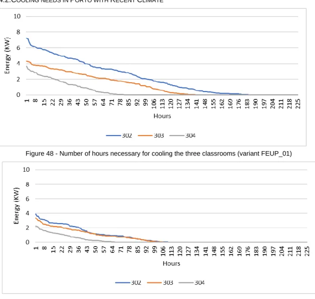
Figure 48 - Number of hours necessary for cooling the three classrooms (variant FEUP_01) ... 44

Figure 49 - Number of hours necessary for cooling the three classrooms (variant FEUP_03) ... 44

Figure 50 - Cooling needs results for the different variants ... 47

Figure 51 – Cooling needs results for the different variants ... 51

Figure 52 - Cooling needs results for the different variants ... 54

Figure 53 - Cooling needs results for the different variants ... 56

Figure 54 – All results of the simulations with cooling considered ... 57

Figure 55 – Cooling needs results of PRG_04 and KB_03 ... 58

Figure 56 - Cooling needs results of PRT_03 and FEUP_03 ... 58

Figure 57 - All simulations considering cooling with Measured climate data ... 59

Figure 58 - Cooling needs results of KB_03 and FEUP_03 ... 60

Figure 59- Average Monthly Temperatures in IWEC Climate in Prague ... 67

Figure 60 - Average Monthly Temperatures in Measured Climate in Prague ... 67

Figure 61 - Average Monthly Temperatures in IWEC Climate in Porto ... 68

Figure 62 - Average Monthly Temperatures in Measured Climate in Porto ... 68

Figure 64 - Indoor air temperatures without considering cooling (PRG_O3 variant) ... 69

Figure 65 - Indoor air temperatures considering cooling (PRG_O3 variant) ... 70

Figure 66 - Indoor air temperatures considering cooling (PRG_O4 variant) ... 70

Figure 67 - Indoor air temperatures in the classrooms without considering cooling (KB_O1 variant) ... 71

Figure 68 - Indoor air temperatures without considering cooling (KB_02 variant) ... 71

Figure 69 - Indoor air temperatures considering cooling (KB_03 variant) ... 72

Figure 70 - Indoor air temperatures considering cooling (KB_03 variant) ... 72

Figure 71 - Indoor air temperatures considering cooling (KB_04 variant) ... 73

Figure 72 - Indoor air temperatures without considering cooling (PRT_O1 variant) ... 73

Figure 73 - Indoor air temperatures without considering cooling (PRT_O2 variant) ... 74

Figure 74 - Indoor air temperatures considering cooling (PRT_O2 variant) ... 74

Figure 75 - Indoor air temperatures considering cooling (PRT_O3 variant) ... 75

Figure 76 - Indoor air temperatures without considering cooling (FEUP_O1 variant) ... 75

Figure 77 - Indoor air temperatures without considering cooling (FEUP_O2 variant) ... 76

Figure 78 - Indoor air temperatures considering cooling (FEUP_02 variant) ... 76

Figure 79 - Indoor air temperatures considering cooling (FEUP_03 variant) ... 77

Figure 80 - Results of PRG_01 simulations with IWEC weather data file... 77

Figure 81 - Results of PRG_02 simulations with IWEC weather data file... 78

Figure 82 - Results of PRG_03 simulations with IWEC weather data file... 78

Figure 83 - Results of PRG_04 simulations with IWEC weather data file... 78

Figure 84 - Results of KB_01 simulations with Measured weather data file ... 79

Figure 85 - Results of KB_02 simulations with Measured weather data file ... 79

Figure 86 - Results of KB_03 simulations with Measured weather data file ... 80

Figure 87 - Results of KB_04 simulations with Measured weather data file ... 80

Figure 88 - Results of PRT_01 simulations with IWEC weather data file ... 81

Figure 89 - Results of PRT_02 simulations with IWEC weather data file ... 81

Figure 90 - Results of PRT_03 simulations with IWEC weather data file ... 82

Figure 91 - Results of FEUP_01 simulations with Measured weather data file ... 82

Figure 92 - Results of FEUP_02 simulations with Measured weather data file ... 83

Figure 93 - Results of FEUP_03 simulations with Measured weather data file ... 83

Figure 94 - Number of hours necessary for cooling the three classrooms (variant PRG_02) ... 84

Figure 95 - Number of hours necessary for cooling the three classrooms (variant PRG_03) ... 84

Figure 97 - Number of hours necessary for cooling the three classrooms (variant KB_03) ... 85 Figure 98 - Number of hours necessary for cooling the three classrooms (variant PRT_02) ... 85 Figure 99 - Number of hours necessary for cooling the three classrooms (variant FEUP_02) ... 85

TABLE INDEX

Table 1 - Simulation cases of Prague, Czech Republic ... 34

Table 2 - Simulation cases of Porto, Portugal ... 34

Table 3 - PRG_01 variation without summer vacations and weekends (without cooling) ... 45

Table 4 - PRG_01 variation without summer vacations and weekends... 45

Table 5- PRG_02 variation without summer vacation and weekends ... 46

Table 6 - PRG_03 variation without summer vacation and weekends ... 46

Table 7 - PRG_03 variation without summer vacation and weekends (without cooling) ... 47

Table 8 - PRG_04 variant without summer vacation and weekends ... 47

Table 9 - KB_01 variation without summer vacation and weekends (without cooling) ... 48

Table 10 - KB_01 variation without summer vacation and weekends ... 48

Table 11 - KB_02 variation without summer vacation and weekends (without cooling) ... 49

Table 12 - KB_02 variant without summer vacation and weekends ... 49

Table 13 - KB_03 variant without summer vacation and weekends ... 50

Table 14 - KB_04 variant without summer vacation and weekends ... 50

Table 15 - PRT_01 variant without summer vacation and weekends ... 52

Table 16 - PRT_01 variant without summer vacation and weekend (without cooling) ... 52

Table 17 - PRT_02 variant without summer vacation and weekends ... 53

Table 18 - PRT_02 variant without summer vacation and weekends (without cooling) ... 53

Table 19 - PRT_03 variant without summer vacation and weekends ... 53

Table 20 - FEUP_01 variant without summer vacation and weekends ... 55

Table 21 – FEUP_01 variant without summer vacation and weekends (without cooling) ... 55

Table 22 - FEUP_02 variant without summer vacation and weekends ... 55

Table 23 - FEUP_02 variant without summer vacation and weekends (without cooling) ... 56

1

INTRODUCTION

Climate Change is an environmental threat but also has a huge impact in economy and energy consumption. We have been witnessing a gradual increase in world’s average temperatures and it is expected that this will continue to influence the increasing energy consumption trends. Recently, it has been an important topic that is being discussed in the building sector, because according to data of Eurostat, this sector is responsible for 40% of final energy consumption in the EU (Europe Union) which means that is among the largest energy consumer sectors, and has a share of 36% in the CO2 emissions related to this sector.

EU Climate & Energy Package and now the 2030 Climate and Energy framework established targets and policy objectives for the period from 2021 to 2030, such as at least 40% cuts in greenhouse gas emissions (from 1990 levels), at least 32% share for renewable energy, at least 32,5% improvement in energy efficiency. So, energy performance of the buildings can play an important role in the achievement of energy savings, with the help of dynamic building energy simulation software, designers and engineers can make energy analysis and predict solutions that can improve energy performance, reducing energy demand, ensure that the optimum indoor thermal comfort and prevent the overheating during the cooling season.

The case study was chosen with the help of the Faculty of Civil Engineering of CTU Prague, and the 3D model was provided by UCEEB (University Centre for Energy Efficient Buildings) and Czech Technical University of Prague. This model was developed in the modelling software Rhino to support the building energy simulations by associating the building elements in the Grasshopper with the actual 3D model. The model was simulated with different variants and with different weather data.

1.2.OBJECTIVE

The objective of this dissertation was to obtain the indoor air temperatures of a school building and the cooling energy needs, that are now increasing with the climate change, this study will also give his humble contribute to demonstrate it. The goal was to study the effect of external shading on the interior temperature of a school building and on cooling energy needs during a school year. The ultimate objective was to obtain the best possible solutions to improve the energy performance of the building. Finally, analyse how the different climatic conditions in Portugal and in the Czech Republic can affect the interior environment of the school.

The goal of this work was also to learn how to use and take advantage of the dynamic building energy engines, in this study the EnergyPlus and Ladybug tools were the tools chosen to perform the energy simulations. This work focus on important aspects such as the impact of solar protection in a building, with the objective of predicting the energy consumption of the building when executing the simulations with Prague standard or recent measured climate and the same for the city of Porto, in Portugal.

1.3.OVERVIEW

This work is divided in 6 chapters which contain the following content:

• Chapter 1 introduces the topic and the framework, defines the objectives of this dissertation and presents its structure.

• Chapter 2 is the State of the art where includes the literature review related to this work, some academic work that already exists that was important to mention such as the background of the building sector, European standards and building physics fundamentals.

• Chapter 3 contemplates the methodology used to produce the simulations results, information about the weather data files for building simulation, explanation of the software used and the presentation of the case study.

• Chapter 4 shows all the results from the building energy software and then the treatment of the data in Microsoft Excel.

• Chapter 5 consists of a discussion on the results displayed in the previous chapter and the analysis on the indoor air temperatures of the classrooms and cooling energy needs of the different variants.

• Chapter 6 is the last chapter where it was referred the main conclusions of this dissertation, and finally some future developments related with the topic.

2

STATE OF THE ART

The building sector is responsible for 40% of final energy consumption in the European Union, which means that is among the largest energy consumer sectors, Data of Eurostat, 2016 shows that 28,1% of national final energy consumption was used just in households in the Czech Republic and 16,3% in households in Portugal [1].

The share of the CO2 emissions in the EU related to this sector is 36%, the average Greenhouse gas emissions in 2016 was 8,7 tonnes of CO2 equivalent per capita, 6,9 tonnes per capita in Portugal and 12,4 tonnes per capita in the Czech Republic [2]. According to Eurostat and a BPIE (Buildings Performance Institute Europe) survey, the average specific CO2 emission in Europe is 54 kgCO2/m2, in 2016 in Portugal was 47 KgCO2/m2 and in the Czech Republic the emission was more than 100 KgCO2/m2 which makes this country having one of the highest CO2 emission per useful floor area in the EU [3]. This can be linked to the energy consumed by heating in the buildings and it is different from country to country. The source of district heating, co-generation and electricity production can be different, and this can affect the CO2 emissions related to buildings.

Energy in households is mainly consumed by heating, cooling, hot water, cooking and appliances, however, the dominant energy end-use in homes is space heating. In terms of final energy use in residential buildings it can be up to 66% in Central/East European countries, of course this depend on different factors such as the performance of the installed heating system, building envelope and climatic conditions. According to ODYSSEE and MURE Databases (Figure 1), in 2015 Portugal’s heating consumption in Kg of oil equivalent was 1.48 koe/m2. On the other hand, Czech Republic was 14.8 koe/m2, which can be mostly explained by climatic conditions but not only [4].

An important share of the residential buildings stock in Europe is older than 50 years and there are a lot Figure 1 - Heating consumption per m², ODYSSEE and MURE Databases, 2015 [4]

group of countries that had a big boom in construction in 1961-1990 and has buildings constructed even before the 1960s when energy building regulations were much different than today. Portugal thanks to mild winters in the Southern European climate the heating needs are lower comparing to the rest of the EU countries.

In the 2016 Proposal for a Directive of the European Parliament and of the Council amending Directive 2010/31/EU on the energy performance of buildings was made an Evaluation of this same Directive. From this document, Evaluation of Directive 2010/31/EU on the energy performance of buildings, Figure 2 shows the annual final energy consumption per square meter in residential sector in EU, Portugal is around 70 kWh/m2 per year and Czech Republic around 240 kWh/m2 per year.

Regarding on non-residential buildings, BPIE divides European buildings in the following categories: wholesale & retail (28%), offices (23%), educational (17%), hotels and restaurants (11%), hospitals (7%), sport facilities (4%), other (11%). This sector account for 25% of total EU floor space building stock, and his annually energy consumption can be quite high, especially in relation to offices, commercial and hospitals buildings, the average energy consumption estimated in these buildings is 280kWh/m2 which is 40% greater than residential sector. This can be explained by the electricity use over the last 20 years, which has increased by 74%, mostly because of technological advances in IT equipment, air conditioning systems, etc. and it is predicted that will continue growing but at a slower pace (1.1% per year) [3].

The building sector is a heterogeneous sector because the characteristics of each building can vary depending on the climate conditions and of the thermal components of the building. Therefore, the energy performance of the buildings can take an important role to achieve important energy savings that were settled by EU Climate & Energy Package, that aims at a 20% increase of energy from renewables, a 20% decrease of greenhouse gases emissions and a 20% reduction of primary energy consumption in

Figure 2 - Latest known annual final energy consumption per square meter in the residential sector (2013 value for all Member States, except (*) 2012 and (**) 2011) [5]

buildings by 2020. These key “20-20-20” targets were already updated by the 2030 Climate and Energy framework that established targets and policy objectives for the period from 2021 to 2030, such as at least 40% cuts in greenhouse gas emissions (from 1990 levels), at least 32% share for renewable energy, at least 32,5% improvement in energy efficiency [6],[7].

In the European Union countries, the main policy driver related to the energy use in buildings is the Energy Performance of Buildings Directive (EPBD, 2002/91/EC). It was recast in 2010 (EPBD recast, 2010/31/EU) and were imposed new requirements for certification, inspections, training or renovation in Member States, so along with this Directive the Kyoto Protocol to the United Nations Framework Convention on Climate Change (UNFCCC) can be followed, that committed to maintain the global temperature rise below 2 °C. This EPBD recast imposes the implementation of energy saving measures for cases of deep renovations of the building. The consequences of the EPBD implementation are already demonstrated for example in Portugal where more than 50% reduction in the U values has been applied over the years [3].

2.2.PORTUGAL AND CZECH REPUBLIC LEGISLATION

The recast of the European Directive had an important role in the new System of Energy Certification of Buildings in Portugal and it is included in the Decree Law 118/2013, as well the complements related to energy performance and calculation methodology in the “Regulamento de Desempenho Energético dos Edifícios de Habitação” (REH) for residential buildings and the “Regulamento de Desempenho Energético dos Edifícios de Comércio e Serviços” (RECS) for non-residential buildings, bringing together all matters on building energy performance in a single law [8].

Moreover, REH applies to residential buildings in the following situations: “design and construction of new buildings; major intervention in the envelope or technical systems of existing buildings; energy assessment of new buildings subject to major intervention and within the framework of the SCE ( Sistema de Certificação Energética dos Edifícios)”, which is the Building Energy Certification System. It shall be checked in the following buildings:“ in case of single-family residential buildings, for the whole building; in case of multi-family residential buildings, for each apartment or in buildings under design or under construction, for each apartment expected; in case of mixed buildings, for fractions intended for housing, irrespective of the application of the REC to the other fractions”. The buildings not intended to housing purpose and special situations are excluded.

The RECS applies to commercial and services buildings in the following situations: “design and construction of new buildings; major intervention in the envelope or technical systems of existing buildings; energy assessment and maintenance of new buildings subject to major intervention and within the framework of the SCE”. The buildings for housing purpose and special situations are excluded. In the RECS it is intended as “interior useful space” as the space that comprises the space partitions that will be included in the calculation of energy requirements for heating purpose as well for cooling to maintain an internal reference temperature of thermal comfort, including spaces that are not usually air-conditioned, such as storage rooms or toilets should be considered as spaces with reference conditions. In the Czech technical standard, ČSN 73 0540-2 Thermal Protection of Buildings the temperature requirements for internal surfaces are now more clearly formulated because it uses the internal surface temperature factor, the design temperature factor must be greater than or equal to the required temperature factor The heat transfer coefficient values of the structures are partially changed and supplemented comparing to the previous standard, this standard from 2011 replaces the previous version of the 2007 standard. The assessment of heat dissipation through the building envelope is adjusted using

For residential buildings, the short-term and limited exceedance of the maximum daily room air temperature setpoint (at most 2 ° C for a maximum of 2 hours) is now permitted in the design phase if the user agrees.

In the Czech Legislation the reference internal air temperature for non-residential buildings is 20 degrees Celsius (⁰C) for Winter and 27 ⁰C for Summer, the Portuguese Legislation has established 20 ⁰C for Winter but for Summer is more severe, which is 25 ⁰C.

These indoor temperature values for summer are set to control the thermal comfort of the indoor environment. For summertime it is related also to prevent the overheating risk during this season. In order to predict if a building will overheat or not, a model of the indoor environment must be developed that represents the specific building by using computer simulation to model the indoor climate. These models must include four important physical parameters: air temperature, radiant temperature, humidity and air movement and information about clothing and activity [10].

2.3.INDOOR CLIMATE

2.3.1.HEAT TRANSFER FUNDAMENTALS IN BUILDINGS

Heat transfer can occur in three modes: Conduction, Convection and Radiation. Conduction is the transfer of heat through a solid or a stationary fluid. It is a transfer of energy from the more energetic to the less energetic particles of a substance due to interactions between the particles. So, in the presence of a temperature gradient, energy transfer by conduction must then occur in the direction of decreasing temperature [11]. In buildings the heat transfer by conduction can be harmful when it happens through building components that have highly conductive characteristics such as windows, although this mechanism occurs in all solid building materials and small air spaces. When designing a building an important situation to be aware is the direct thermally connections between the inside and outside of the building, usually defined as thermal bridge. A thermal bridge is a localised area of the building envelope where the heat flow is different, usually increased, in comparison with adjacent areas, so this can alter the heat conduction of the building envelope, increase heat losses and usually decreased interior surface temperatures [12].

Convection is the transfer of heat energy between a fluid in motion and a bounding surface when the two are at different temperatures, in buildings this mechanism happens inside the structure of the building materials, unventilated air spaces, windows and other ventilations inlets and unwanted cracks in the building. This is an important aspect when designing buildings, because of the essential interior ventilation to mix fresh air to control the internal temperatures of the buildings. It is also relevant for the prevention of accumulation of moisture[11][12].

Radiation is the transfer of heat energy by electromagnetic waves. While the transfer of energy by conduction or convection requires the presence of a material medium, radiation does not. In buildings one of the natural events that influences the indoor environment is the incident solar radiation in the building and the heat exchange that occurs with the outside environment. Inside the building there is also the heat exchange between all the surfaces of the building and the heat exchange from a radiant heat systems [11][12].

2.3.2.THERMAL COMFORT

The optimal situation is when the person is in thermal equilibrium with the environment as the energy transfers between the body and the surroundings are equal. However, in the work of Fanger was proposed a balance between the heat produced by the body and the heat lost from it as a necessary, but

not sufficient, condition for thermal comfort. It is not sufficient because it is possible to accomplish physical balance and not be comfortable (for example, where there is a big asymmetric radiant source such as a cold window). Therefore the determination of comfort conditions is in two stages: first detect the conditions for thermal balance and then determine which of the conditions so defined are consistent with comfort [13]. So as Fanger shows in his work developed on thermal comfort, the conditions of thermal comfort are ruled by the following set of variables: the three individual factors such as metabolism, skin temperature of the individual, clothing, then the other four Ambiental factors such as air temperature, mean radiant temperature, relative humidity and air velocity.

The air temperature is the most important parameter, as well as the radiant temperature, both generate the temperature of environment that is surrounding the human body and it affects the heat loss from the body by convection, when higher the heat produced by the body through metabolism will suffer less losses and the other way around [13].

2.4.EUROPEAN STANDARDS FOR ENERGY PERFORMANCE OF BUILDINGS

The radiant temperature is the mean radiant temperature which is the “uniform surface temperature of an enclosure in which an occupant would exchange the same amount of radiant heat as in the actual non-uniform enclosure” [14]. The radiant temperature can also have a distinct directionality, such as when there is a radiant heater, a cold window or direct sunlight.

The air and radiant temperatures are combined to give the operative temperature, which models the combined effect of convective and radiant heat exchange. In EN ISO 52017-1 [14], operative temperature is defined as “uniform temperature of an enclosure in which an occupant would exchange the same amount of heat by radiation plus convection as in the actual non-uniform enclosure”. The operative temperature is calculated according to Equation (1):

θop = fa θa;i +(1- fa)θmrt (1)

Where,

θop is the operative temperature, in °C;

fa is the fraction that the air temperature contributes to the operative temperature;

θa;i is the temperature of the internal air, in °C;

θmrt is the mean radiant temperature, the weighted average of internal surface temperatures, in

°C, calculated according to Equation (2):

θmrt = ∑ (𝐴𝑗.𝜃𝑠,𝑗) 𝑗

∑ 𝐴𝑗𝑗 (2)

Where

θs,j is the internal surface temperature of building element j Aj is the area of building element j, in m2.

In a top-quality building in winter, most of the surfaces are close to air temperature and the air temperature (Ta) can be equal to operative temperature (Top). However usually with sunny weather

Top ≈ (Tr + Ta) / 2 (3)

Where

Tr is the radiant temperature, in °C;

The EN ISO 52017-1 standard cancels and replaces EN ISO 13791 and the main differences are the calculation of the operative temperature explained before, some assumptions or procedures that are not relevant for the generic calculation procedures have been moved to the standard specific application and vice-versa, the heat flow rates due to energy needs for heating and cooling and due to energy needs for (de-) humidification are added to the formulae[14][15]. This makes the application range of the generic calculation procedures much wider, without adding complexity, because these heat flow rate terms are identical to the heat flow rate terms due to internal sources. How to calculate the heat flow rates due to energy needs for heating and cooling is not explained in this standard, but in the specific application standard ISO 52016-1 [16].

For the EN ISO 52017-1 some assumptions were made for the calculation of the internal temperatures such as the air temperature is uniform throughout the building zone; the various surfaces of the building elements are isothermal; the heat conduction through the building elements (excluding to the ground) is assumed to be one-dimensional; the heat conduction to the ground through building elements is treated by an equivalent one dimensional heat flow rate according to ISO 13370; the heat storage contribution of (linear or point) thermal bridges is neglected; (linear or point) thermal bridges are directly thermally coupled to the internal and outdoor air temperatures; air spaces are treated as air layers bounded by two isothermal and parallel surfaces; the heat storage effects in the various planes of a glazed element are neglected; the density of heat flow rate due to the short-wave radiation absorbed by each plane of a glazed element is treated as a source term [17].

EN ISO 52016-1 and the technical report CEN ISO/TR ISO 52016-2 contain a simplified hourly calculation method and a monthly calculation method for the calculation of the sensible energy need for heating and cooling and the latent energy need for (de)humidification. This standard cancels and replaces EN ISO 13790 [18]. The method in the EN ISO 52016-1 adapted boundaries conditions and simplifications so that the input data can get the calculation of internal temperatures without cooling for summer conditions and without heating for winter and calculation of both loads.

These documents give calculation methods for the assessment of the (sensible and latent) energy load and need for heating and cooling and the internal temperature based on hourly calculations. The specific hourly method can calculate the indoor air, mean radiant and operative temperature, it also includes a specific hourly method to calculate the moisture and latent energy loads and needs for humidification and dehumidification and hourly indoor air moisture content. The calculations are done per each thermal zone defined as “internal environment with assumed sufficiently uniform thermal conditions to enable a thermal balance calculation according to the procedures in the standard under EPB module M2-2”, M2 is the “Building” module main area and M2-2 is the submodule “Building Energy Needs”. The hourly and the monthly method in EN ISO 52016-1 are linked as they use as much as possible the same input data although the hourly method can produce more output at the same time because also can get the key monthly quantities needed to generate parameters for the monthly calculation method. This method is a specific application of the generic method that is contained in EN ISO 52017-1 and is more advanced than the simplified hourly, three node (5RC1) method in the EN ISO 13790 because the building elements are not aggregated to a few lumped parameters, but kept separate in the model, as its illustrated in the Figure 3[17][18]

Figure 3 - Improved hourly method in EN ISO 52016- 1 (b) compared to simplified method in EN ISO 13790:2008 (a) [16]

These changes makes the model more transparent and more widely usable compared to EN ISO 13790 considering that the combination of for example the heat flow through the roof and through the ground floor is possible to consider although they have such a different environment conditions (ground temperature and ground inertia, solar radiation on the roof). The thermal mass of the building can be specified per building element and this parameter is not arbitrary lumped anymore into a single overall thermal capacity for the building and the mean radiant temperature can be accurately identified and distinct from the indoor air temperature.

In this hourly calculation method, the thermal balance of the building is made up at an hourly time interval so comparing to the monthly method it can be take into account the influence of hourly and daily variations in weather, operation of solar blinds for instance and occupation. The drawback is that it needs a much more robust numerical software because of his higher number of nodes. The RC model adopted in EN ISO 52016-1 is more advanced and consists of 5 nodes per building element and a capacitance for each building element inside a thermal zone [16].

An accompanying spreadsheet was produced on EN ISO 52016-1, covering both the hourly and the monthly calculation method and it is on the Part 2. No spreadsheet was produced on EN ISO 52017-1, because this EPB standard (with reference hourly thermal balance calculation procedures) is not directly used for calculations.

Usually all EPB standards follow specific rules that ensure some consistency, unambiguity and transparency, although these standards provide quite flexibility in the methods because of the differences in some national and regional level and their climatic conditions, legislation and policies and technology. That can be found in the normative template in Annex A and Annex B in EN ISO 52016-1 and the

information related with the input data, this is important because of the application of the different building regulations for energy performance and requirements.

2.5.OVERHEATING RISK

One of the causes of overheating is the heat that comes from the solar gains through the building fabric (roof, external walls, windows, doors, lowest floor), although in modern buildings the heat conducted through the opaque elements of the building is not so substantial comparing to older buildings when the insulation has not been upgraded. The other source of heat is the solar gains that comes from the direct gains through glazing can be highly significant, mainly in the windows that are facing orientations between South and West. Therefore, shading systems, blinds and curtains may have an important role as they can reduce these direct gains if placed correctly.

Also, the external air temperature can be a significant cause because when this temperature is higher than indoor temperature can, for example, be brought into the building from the ventilation and increase the indoor air temperature. The last cause of overheating it is related with the internal heat gains, not only the common activities such as cooking, bathing, etc. but just the heat emission from the occupants inside the building.

From a practical perspective Nicol et al. [19] in his studies acknowledge that the criteria of overheating evaluation “is determined by both the building category and the mean external dry bulb temperature for a number of previous days, then the measurement and ultimate determination of overheating becomes more complex”.

CIBSE Guide A defined overheating as occurring when the operative temperature exceeds 28 ⁰C for more than 1% of the annual occupied hours in the living areas of dwellings or when the bedroom operative temperature exceeds 26 ⁰C for more than 1% of the annual occupied hours. Some problems can occur when a threshold temperature is fixed and also hours over standard such as this one because this temperature even in UK can be considered acceptable in a warm UK Summer or any other country. Other way to define overheating is to identify a particular temperature above which a given proportion of people in a building (for example 20%) vote +2 or +3 on the ASHRAE scale, that includes +3 Hot, +2 Warm, +1 Slightly warm, 0 Neutral, –1 Slightly cool, –2 Cool, –3 Cold [20][21].

It is noticed that in Summertime the cooling needs in some countries can be really high due to the solar radiation through highly glazed building façades. These surfaces of modern buildings with direct exposure to the sun through windows, walls and roofs can be problematic as they admit heat from solar radiation, this leads to an increase in the amount of energy [22].

2.6.MEASURES TO PREVENT OVERHEATING

Studies performed before showed the great importance of the internal gains on the cooling loads and some measures can be contradictory, for example it is possible to reduce these internal gains with the better use of daylighting, although there is a need to be careful when increasing glazed surfaces and the orientation of the windows. To ensure that the design is futureproof, the overheating risk in future climates is already being the focus of some studies given that mean external temperatures and solar insolation are expected to increase with a warming climate [23].

Ventilation can have a relevant influence in this matter as can control the indoor temperature of a building in Summer, especially if it is taken advantage of the night ventilation, which is in theory less expensive. Architectural design must be aware and from early stage think in strategies such as cross-ventilation for natural cross-ventilation or chimney effects. Thermal inertia is also an essential aspect for night

ventilation and to reduce temperature rise inside, the increasing of thermal mass reduces overheating and temperature fluctuation [24]. Are now being used phase change materials like paraffins and salt hydrates as mechanisms for heat transfer in building because when they change phase, they absorb or release significant amounts of heat energy. So, these materials can reduce internal temperature changes by storing latent heat in the solid-liquid or liquid-gas phase change, PCMs (phase change materials) used in buildings will typically melt and solidify within a range of 18-30ºC. They can store up to 14 times more thermal energy per unit volume than conventional thermal storage materials [25].

The use of solar shading devices is another way to solve the overheating and also the glare problems in modern buildings. To avoid the inflow of heat, the surfaces on which the sun’s rays fall must be protected. Shading devices can protect glazed windows from allowing the penetration of incoming heat and consequently increase the risk of overheating [26][26]. The position of solar shading systems can be fixed or movable (manual or automatic) with different classification of systems such as external, intermediate or internal and different types such as overhangs, horizontal louvers, vertical louvers, side-fin, blind system like venetian blinds and a more complex combination of vertical and horizontal elements, egg-crate shading (Figure 4). There are also possibilities like the combination of fixed and movable shadings, shading devices integrating a solar thermal system, building-integrated photovoltaic shading-type, combination of electrochromic windows and overhangs [27].

2.7.KÖPPEN-GEIGER CLIMATE COMPARISON

In the first instance, one evident approach could be the comparison trough the well-known empirical method Köppen-Geiger classification. Which is a system based on observation of air temperature and precipitation, this system classifies climate into five main classes and 30 sub-types. It is possible to analyse different regions with similar characteristics. The Figure 5 demonstrates the climate differences between the European countries, where is located Czech Republic and Portugal.

Figure 5- Europe map of Köppen-Geiger climate classification [28]

In the Figure 6 it is presented the 2 Portuguese climate zones, Csa (warm Mediterranean) in the south and Csb (temperate Mediterranean) in the north. The Mediterranean climate or dry summer climate is characterized by rainy winters and dry summers, with less than 40 mm of precipitation for at least three summer months. The average annual temperature in continental Portugal is 14.7°C but varies from 4 °C in the north-eastern to 18 °C in the south [29].

In this study the Portuguese city that is on focus is Porto, the autumn and winter are typically windy, rainy and cool, as it is cooler in the northern and central districts of the country. However, in the southernmost cities of Portugal, temperatures only occasionally drop below 0 °C, remaining at 5 °C in most cases.

Figure 6 - Portugal map of Köppen-Geiger climate classification

The climate of the Czech Republic can be defined as typical European continental climate, most of the country is classified Dfb (temperate continental climate), having warm, dry summers and fairly cold winters, but there is also some small areas classified as Dfc (cool continental climate) and Cfb (temperate oceanic climate) as shown in the Figure 7. The temperature difference between summer and winter is relatively high, due to the country be a landlocked country, nights can be quite cool even in summer, which is also significant climate characteristic. The average annual temperature in the Czech Republic is 8ºC and the precipitation is rather low, just over 500 mm per year, but it fluctuates in dependence on geographic factors between 1.1 to 9.7 °C [29].

In Prague, the winters are relatively cold with average temperatures at about freezing point, and with very little sunshine. The month of January is the coldest month with daytime temperatures usually around zero, although summers have an average high temperature of 24 °C. Prague represents a specific region, as within its heat island the average annual temperatures higher by approximately 1 to 2°C above the value normal for its geographic location.

Regardless of considerable year-to-year fluctuations, there is an apparent trend of gradual rise in average annual temperature amounting to approximately 0.2°C over 10 years in the Czech Republic and in Portugal since the mid-70s the average temperature has risen in all regions of Portugal at a rate of approximately 0.3°C per decade [29] [30].

3

METHODS

The main goal of this study is to analyse how the climatic conditions of two different countries such as Portugal and Czech Republic can affect the indoor environment of one school building during the school calendar year. The case study chosen is a real school building and to evaluate this building it was used a 3D model provided by Civil Engineer faculty of CTU Prague.

This model was developed before in the modelling software Rhino to support the energy simulations by associating the building elements in the Grasshopper with the actual 3D model. The methodology used to achieve the necessary cooling loads to maintain thermal comfort inside the building is explained in the following points, for this study it was consider the evolution of the standard climate to the recent climate, changing the inherent variables and then creating different simulations cases.

Through the usage of energy simulation software that are enclosed in Ladybug Tools in Grasshopper, such as EnergyPlus, it is possible to predict energy consumption, indoor air temperatures, needs for heating and cooling, consumption needs of HVAC (Heating, ventilation, and air conditioning) systems, levels of ventilation. However, the target of this work was the cooling season and ways to prevent the overheating risk, so the goal was to obtain the indoor air temperatures of the building and cooling energy needs, although the cooling demand in buildings usually is lower than heating demand, is now increasing with the climate change.

3.2.CLIMATE ANALYSIS

3.2.1.HISTORY OF WEATHER FILES FOR BUILDING SIMULATION

Weather data is used in the building industry to assess the performance of the building in a potentially environment, when developing the design at the early stage of construction. This topic is becoming critical because climate change is leading to unwanted extreme weather events and can really influence the built environment [31] .

Dynamic building energy simulations started in the earlies 1950s, although they were only improved in the 1970s because of the petroleum energy crisis in United States of America and western Europe, after that it could really be used as a tool to improve the energy performance of buildings [32]. In these first models, weather data were applied to a software in different formats and they were later standardised into “weather files” by the third generation of dynamic building simulators, following the classification of Clarke that acknowledge that regardless of the source of weather data, a collection (usually annual) must be classified in terms of its severity. These files should take a form of typical weather years, created from hourly observed measurements at a specific location [33].

So there is a need now to start to think in ways to adapt the buildings to the impacts of future climate change, this problem has already created a requirement to incorporate climate change projections into these weather files, either by modify the weather data or synthetically generating it [34].

3.2.2.BACKGROUND OF HOURLY WEATHER DATA FILES

sponsored by the Department of Energy from United States of America. The popularity of EnergyPlus has driven the popularisation of its native weather file format “.epw” file (Energy Plus Weather). These .epw files are text-based CSV (comma-separate values) and they have years’ worth of hourly weather variables for a location [35].

Usually this type of file consists of 8760 rows for every hour of the year, and columns with parameters describing the weather such as following: time, outdoor air temperature, humidity, wind direction, wind speed, direct radiation and diffuse radiation.

Weather data files can be classified in three main classes:

• Typical Meteorological Year (TMY), typical weather data representative of some specific location over a longer period of time (e.g. 30 years).

• Actual Meteorological Year (AMY). Actual weather data of a specific site and year. • Future (forecast) weather data used for adaptive control of buildings.

The TMY or TMY3 (last version) weather data files are used around the world for design and performance conditions over the life of a building, in these class the commonly used worldwide is the IWEC files. Although these TMY files have different sources or ways to create them, several of them use common file formats such as the EPW format. The file itself consists of months selected from individual years, then assembled to form a complete year computed using the Finkelstein-Schafer (FS) statistic, this means that each month in the file might be from a different year [35].

There is also another type of file that is called the Test Reference Year (TRY), that is commonly use in the UK, the Chartered Institution of Building Services Engineers (CIBSE) in association with the UK Met Office produces TRYs for the United Kingdom. These files contain hourly data of climate characteristics like outdoor temperature, solar radiation, relative outdoor air humidity, wind speed and direction, quantity of rainfall, composing 12 months of data, each one chosen to be the most average month among a set of years made up of the daily mean of values of dry bulb temperature, cloud cover and relative humidity (component months are chosen using the same statistic method than TMY). In the last update [36] there were made some changes in the parameters to use dry bulb temperature, cloud cover, and relative humidity as primary variables with wind speed as a secondary variable.

In Europe, the Meteonorm system (Meteonorm 2000) is an extensive source of weather data with 2400 meteorological stations worldwide and also a weather generator. The radiation database - a mixture of ground and satellite data – includes long term monthly averages. Daily, hourly or minute values are generated stochastically [33].

3.2.3.IWEC WEATHER FILES

IWEC stands for International Weather Year for Energy Calculation and it was released in 2000 by American Society of Heating, Refrigerating and Air-Conditioning Engineers (ASHRAE) as an attempt to unify all the international weather files. The goal of ASHRAE was using the Integrated Surface Hourly (ISH) weather data to produce as many “typical year” weather files as possible, then release them in a similar format to TMY3. IWEC files contain weather observations of wind speed and direction, sky cover, visibility, dry bulb temperature, dew point temperature, atmospheric pressure, liquid precipitation, and current weather for at least 12 years of records but up to 25 years. Information on solar radiation sometimes is estimated on an hourly basis from earth-sun geometry and hourly weather elements such as cloud cover and type, if the ISH data does not have enough measurements.

Version 2 of IWEC or IWEC2 is now the ASHRAE’s current weather format and much more developed. The data are derived from meteorological reports from over 3,000 international locations. This current version has lower weights for global horizontal radiation but higher weights for direct normal solar radiation than the previous version [37].

3.2.4.WEATHER DATA CHOSEN FOR THE SIMULATIONS

With the previous topics taken into consideration, it was decided that should be done a variety of different simulations with standard weather data and recent weather data of Prague, Czech Republic and of Porto, Portugal. So, the weather data serving as standard climate for the simulations in both cities is the IWEC file available in the Energy plus website. For the most recent possible and available weather data, both data were provided by the two universities, UCEEB of CTU Prague and FEUP (Faculty of Engineering-University of Porto), to be used in this study.

For the most recent weather data of Prague it was used an actual measured data that was acquired by the UCEEB of CTU Prague. The solar radiation data was the only parameter taken from the city centre because the rest of parameters are from Kbely airport, this data was collected in the year of 2018. The Kbely airport was also chosen especially because is far away from the city centre and the data does not contain the possibility of urban heater island effect, which is when the city centre is significantly warmer than its surroundings. The weather data used as recent weather climate of Porto was a file created by actual measurement of the parameters in FEUP, Porto, this file is an artificial annual year based on the interpolation of data collected in the past eight years and then this annual year can include maximum and minimum values that were not even from the same year. All of these measured data was used to create a .epw data files format because it is the necessary format to import weather data to the Grasshopper in the Rhino software with the Ladybug tools.

Figure 9- Typical Meteorological Year Porto (IWEC data)

These two figures, Figure 8 and Figure 9, represent the typical meteorological year of both cities in study, these two data files were the first climate used in the simulations of each city, the weather data IWEC file is created with at least 12 years of records, the one from Prague is from 1995 and the one from Porto is from 1993. It is worth to make a brief analysis of how the temperatures fluctuates during the year, the maximum outdoor air temperature in the IWEC weather data of Prague is 32,00ºC during all year but it is 27,50ºC if the summer period was not considered. For the measured weather data in Prague the maximum outdoor air temperature is 35,00ºC during all year and if summer period was not considered is 30,00ºC. The differences between the temperatures from the IWEC weather data and the measured data, at least a 2,5ºC rise in the recent maximum temperature if the summer period was not taken into account.

The maximum outdoor air temperature in the IWEC weather data of Porto is 32,00ºC during all year but it is 29,90 ºC if the summer period was not considered. For the measured climate in Porto the maximum outdoor air temperature in the is 36,40ºC during all year but it is 34,90ºC if the summer period was not considered. Comparing to the weather data of Prague, the differences are even more clear between the both weather data of Porto, thanks to the 4,4ºC rise in the recent maximum temperature and 5ºC if the summer period was not taken into account.

Figure 10- Weather Data Measured in Prague

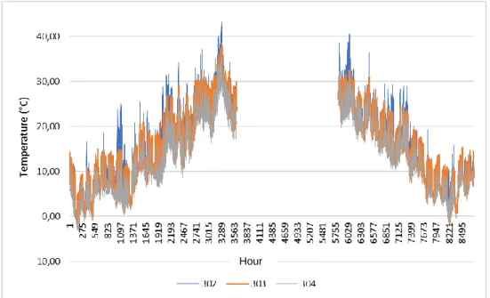
In these two figures, Figure 10 and Figure 11, are the weather data that was measured in Prague and Porto, and it is important to mention the differences between the IWEC weather data of Prague and this recent measured data, as the maximum and minimum temperatures during all year are higher and lower values and this is more clear in the Figure 12 and Figure 13.

Since this type of chart sometimes is not the best to get a clear overview on the average monthly temperatures, this subchapter is also provided with charts with the average monthly temperatures isolated in order to give to the reader a simple way to present the data.

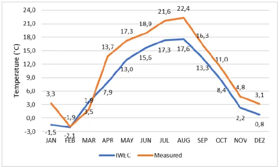
Figure 12- Comparison of Average Monthly Temperatures of IWEC and measured data in Prague

The simulations were performed not only to compare the differences between the both cities but also to see the contrast of the recent measured data with the IWEC data, as its shown in the Figure 14 and Figure 15, and this will influence the results of the simulations.

Figure 14 - Comparison of IWEC data between Prague and Porto

Figure 15 – Comparison of measured data between Prague and Porto

One of the main important input for the simulations that were performed is the outdoor temperatures (dry bulb temperatures), but also the solar radiation can have an important role in the obtained results. In the next four figures ( Figure 16, Figure 17, Figure 18 and Figure 19) it is possible to compare the normal solar radiation between different climates for the same city and between both cities, which is the variable with more weight in the simulations.

Figure 16 - Comparison of Normal Solar Radiation in Prague

Figure 18 - Comparison of normal solar radiation between Prague and Porto (IWEC Data)

Figure 19 - Comparison of radiation between Prague and Porto (Measured data)

3.3.SOFTWARE USED

EnergyPlus, current version 9.1.0, was the chosen software for this study and is a whole building energy and thermal load simulation engine that uses a system that controls several modules, which communicate using simple and clear information exchange (plain text files). It is one of the most known energy simulation software tools in the world, consequently engineers, architects, and researchers usually use to model both energy consumption—for heating, cooling, ventilation, lighting and plug and process loads—and water use in buildings [37].

EnergyPlus development started in 1996, sponsored by the Department of Energy (DOE) from USA, it is a modular, structured code based on the most popular features and capabilities of BLAST and DOE-2.1E, both abandoned software by DOE but were the first step and the working basis of the Energy Plus,

which works with input and output of text file, however is an entirely new software tool that combines the heat balance of BLAST with a generic HVAC system.

One of the best features achieved by this software was the integration of all aspects of the simulation loads, systems, and plants. In this integrated (simultaneous) simulation software the loads calculated (by a heat balance engine) at a user-specified time step (15-minute default) are passed to the building systems simulation module during the same time step. Therefore, it calculates heating and cooling system and plant and electrical system response. The diagram in the Figure 20 shows an overview of the integration of these important elements of a building energy simulation.

Integrated simulation enables the possibility to evaluate realistic system controls, moisture adsorption and desorption in building elements, radiant heating and cooling systems, and interzone air flow [38]. It is important to mention that in Energy Plus does not exist a visual interface that allow users to see and concept the building, so it was relevant to use a software where it was possible to associate the data used in EnergyPlus with a 3D model software like Rhino, which its linked with Grasshopper. Grasshopper is the graphical user interface chosen for this work, the GUIs uses visual programming language and it is in his interface where the interoperability between the tools is possible. Inside the Grasshopper software it is possible to make connections with different plug-ins that helps the users generate parametric models based on algorithms for architecture and design.

Therefore, for this study I decide to use the Ladybug Tools (Grasshopper plug-in) which runs within 3D modelling software Rhino and allows data transfer between its simulation engines, not only an energy performance software, EnergyPlus, but a vast amount of applications where it is possible to connect with EnergyPlus inside of Grasshopper. Ladybug Tools basically is a collection of free computer applications related with environmental design, the first version was released on January 2013 and it started to be a collection of 28 components for weather data visualization, solar radiation studies, and sunlight hours analysis. Following the success of Ladybug, the developers released Honeybee for Grasshopper in 2014 to connect Grasshopper to validated daylighting and energy simulation engines, such as RADIANCE, Daysim, EnergyPlus and OpenStudio. Since this release, these tools have been admired by the users as the plug-in is at the moment the third most popular plugin for Grasshopper [37].

They are currently linking Ladybug Tools with more analysis engines such as the Urban Weather Generator, and the SyntheticWeather engine for climate change projections, the plug-in name is Dragonfly, which they continue adding features.

To ensure the long-term sustainability of the project as it grows exponentially, Mostapha and Chris co-founded Ladybug Tools LLC in August 2017 to deal with all the commercial services around the project, such as project consulting, cloud computing, and training.

Because it is a free and open source interface, throughout this time, many developers contributed to the community in many ways. As a result of their efforts, Ladybug Tools has grown into multiple inter-connected libraries and plugins that are used in education as well as architecture and engineering offices worldwide. So, with these tools it is possible to import weather files (.epw) from EnergyPlus to Grasshopper or Dynamo and support the engineers design process during early stages by easily making 2D and 3D interactive climate graphic, Ladybug also supports the evaluation of initial design options through solar radiation studies, view analyses, sunlight-hours modelling, and more as shown in Figure 21 [39].

Figure 21 -Interoperability of Ladybug Tools [39]

The Honeybee tool was created for more detailed daylighting and thermodynamic modelling, which frequently is most relevant during mid and later stages of building design. It is appropriate to create, run and visualize the results of daylight simulations using Radiance, also valuable to run energy models by using different plug-ins such as EnergyPlus or OpenStudio, including the possibility of testing shading devices and anticipate the benefits of exterior shade to decrease cooling energy use while not affecting heating energy use. All of these tools are available in the ladybug and honeybee tabs of the Grasshopper interface which are shown in the Figure 22, and the user only has to select and drop them on the canvas.