Automatic transcription of music using deep learning techniques

(1)

Dissertation

Master in Computer Engineering – Mobile Computing

Automatic Transcription of Music using

Deep Learning Techniques

André Ferreira Gil

(2)

(3)

Dissertation

Master in Computer Engineering – Mobile Computing

Automatic Transcription of Music using

Deep Learning Techniques

André Ferreira Gil

Dissertation developed under the supervision of Professor Carlos Fernando Almeida Grilo, Professor Gustavo Miguel Jorge Reis and Professor Patrício Rodrigues Domingues, from the School of Technology and Management of the Polytechnic Institute of Leiria.

(4)

(5)

III

Acknowledgements

First of all, I would like to thank my supervisors, Prof. Carlos Grilo, Prof. Gustavo Reis and Prof. Patricio Domingues, for all their advice, support, guidance and patience throughout this dissertation. Without them this work would have been unfeasible.

Also I would like to thank the Polytechnic Institute of Leiria for giving me the opportunity to study in an amazing school that is comprised by competent staff who strive daily to prepare students for the future.

In addition, I am very grateful to my family and friends who have helped directly and/or indirectly in this work, from financial aid to psychological encouragement.

Lastly but not less important, I would especially like to thank my girlfriend, Maria Angeles, for all the support and patience during all this journey.

(6)

IV

(7)

V

Previous note

(8)

VI

(9)

VII

Resumo

A transcrição de música consiste em identificar as notas musicais ao longo duma música. Esta é uma tarefa árdua que geralmente requer pessoas com muitos anos de treino. Devido à sua enorme dificuldade, tem havido um grande interesse em automatizar esta tarefa. No entanto, a transcrição automática de música engloba vários campos de pesquisa, tais como o processamento sinal, aprendizagem de máquina, teoria musical e cognição e percepção de pitch e de psicoacústica. Deste modo uma possível solução ao problema torna-se difícil de encontrar.

Neste trabalho é apresentado uma nova abordagem de transcrição automática de música de piano usando técnicas de aprendizagem profunda. Tiramos proveito deste tipo de técnicas para criar vários classificadores, sendo cada um deles responsável por identificar uma única nota musical. Em teoria, esta técnica de divide to conquer pode permitir melhorar a capacidade de transcrição de cada classificador.

É de realçar que também são aplicadas duas etapas adicionais denominadas por, pré-processamento e pós-pré-processamento, com o intuito de aperfeiçoar a eficiência do nosso sistema. A fase de pré-processamento visa aumentar a qualidade dos dados de entrada antes de iniciar o processo de classificação, enquanto que a fase de pós-processamento visa em corrigir erros originados durante a fase de classificação.

Inicialmente, foram realizadas experiências preliminares de modo a otimizar o nosso modelo final ao longo das três etapas: pré-processamento, classificação e pós-processamento. O modelo resultante é finalmente comparado com outros dois trabalhos recentes que utilizam tanto a mesma técnica de inteligência artificial como também o mesmo conjunto de dados de treino e teste, mas com outro tipo de abordagem. A abordagem utilizada por estes trabalhos consiste em criar uma única rede neuronal responsável em identificar todas a notas musicais, em vez de uma rede neuronal por cada nota. No fim, é demonstrado que a nossa abordagem é capaz de superar os dois outros trabalhos em métricas de frame-based e ao mesmo tempo, alcançar resultados similares em métricas de onset only, demonstrando assim a viabilidade da abordagem.

Palavras-chave: Transcrição Automática de Música, processamento de sinal

digital, redes neuronais artificiais, aprendizagem computacional e aprendizagem profunda.

(10)

VIII

(11)

IX

Abstract

Music transcription is the problem of detecting notes that are being played in a musical piece. This is a difficult task that only trained people are capable of doing. Due to its difficulty, there have been a high interest in automate it. However, automatic music transcription encompasses several fields of research such as, digital signal processing, machine learning, music theory and cognition, pitch perception and psychoacoustics. All of this, makes automatic music transcription an hard problem to solve.

In this work we present a novel approach of automatically transcribing piano musical pieces using deep learning techniques. We take advantage of deep learning techniques to build several classifiers, each one responsible for detecting only one musical note. In theory, this division of work would enhance the ability of each classifier to transcribe. Apart from that, we also apply two additional stages, pre-processing and post-processing, to improve the efficiency of our system. The pre-processing stage aims at improving the quality of the input data before the classification/transcription stage, while the post-processing aims at fixing errors originated during the classification stage.

In the initial steps, preliminary experiments have been performed to fine tune our model, in both three stages: pre-processing, classification and post-processing. The experimental setup, using those optimized techniques and parameters, is shown and a comparison is given with other two state-of-the-art works that apply the same dataset as well as the same deep learning technique but using a different approach. By different approach we mean that a single neural network is used to detect all the musical notes rather than one neural network per each note. Our approach was able to surpass in frame-based metrics these works, while reaching close results in onset-based metrics, demonstrating the feasability of our approach.

Keywords: Automatic Music Transcription, multi-pitch estimation, digital signal

(12)

X

(13)

XI

List of acronyms

AI - Artificial intelligence.

AMT - Automatic music transcription. ANN - Artifical neural network.

CGP - Cartesian genetic programming. CNN - Convolutional neural network. CSV - Comma Separated Values. DFT - Discrete Fourier Transform. DSP - Digital signal processing. F0 - Fundamental frequency. FFT - Fast Fourier Transform. GA - Genetic algorithm. HMM - Hidden Markov Model. Hz - Hertz.

JPEG - Joint Photographic Expercts Group. KHz - Kilohertz.

MIDI - Musical Instrument Digital Interface. NMF - Non-negative matrix factorization. RNN - Recurrent neural network.

STD - Standard deviation.

STFT - Short-Time Fourier Transform. SVM - Support vector machine. URL - Uniform Resource Locator.

(14)

XII

(15)

XIII

List of figures

Figure 1.1 - The two main tasks of the transcription process ... 1

Figure 1.2 - Common approach for pitch estimation process... 2

Figure 1.3 - Monolithic process for transcribing musical notes ... 3

Figure 1.4 - Multiple classifiers, each one responsible for detecting a specific musical note ... 3

Figure 2.1 - Representation of the oscillations generated by a sound ... 6

Figure 2.2 - Comparison of a continuous and a discrete signal ... 6

Figure 2.3 - Low sampling rate problem ... 7

Figure 2.4 - An example of a digital sound that follows the Nyquist theorem ... 7

Figure 2.5 - Digital signal with a bit depth of 2 ... 8

Figure 2.6 - Three examples of periodic signals ... 9

Figure 2.7 - Representation of a quasi-periodic signal. This sound was generated by a virtual piano software, playing the note E1. ... 9

Figure 2.8 - Low and high frequency representation... 11

Figure 2.9 - Example of both the Fourier analysis and the Fourier synthesis processes ... 11

Figure 2.10 - A comparison of the same sound in two different domains ... 14

Figure 2.11 - Representation of the spectral leakage event ... 15

Figure 2.12 - An example of missing fundamental resulting at 300 Hz ... 16

Figure 2.13 - Representation of a monophonic signal ... 18

Figure 2.14 - Representation of a polyphonic signal ... 18

Figure 2.15 - An example of the spectral envelope ... 20

Figure 2.16 - Representation of a biological neuron ... 23

Figure 2.17 - Representation of an artificial neuron ... 23

Figure 2.18 - Representation of an ANN with a single hidden layer ... 24

Figure 2.19 - Representation of a multi-layer neural network ... 24

Figure 2.20 - Example of a linear and a non-linear problem ... 26

Figure 2.21 - Representation of several activation functions ... 27

Figure 4.1 - Overall architecture of the proposed model ... 41

Figure 4.2 - Representation of the main steps during the pre-processing stage ... 42

(20)

XVIII

Figure 4.4 - Example of positive, negative or silence frames, regarding the musical note D4 ... 43 Figure 4.5 - Representation of all the transformations that occurs during the data transformation step in the pre-processing stage ... 43 Figure 4.6 - Representation of the main steps that happen during the classification stage . 44 Figure 4.7 - Representation of the structure of a single step in the post-processing stage . 45 Figure 4.8 - Representation of the all three steps that are taken during the post-processing stage ... 46 Figure 4.9 - Example of how the step 1 from the post-processing stage works ... 47 Figure 4.10 - Representation of all the sequences given to the post-processing step 1 and its resultant transcription ... 48 Figure 4.11 - Representation of the three types of sequences, received by the post-processing step 2 ... 49 Figure 4.12 - Representation of a perfect onset detection and a more likely output from our onset algorithm ... 50 Figure 4.13 - Representation of the three possible transformations that could occur in this post-processing step ... 51 Figure 4.14 - Illustration of the given input data in an ideal scenario, with all the three types of possible predictions ... 52 Figure 4.15 - Representation of the difference on how different predictions, from step 3, could affect the resultant transcription ... 53 Figure 4.16 - Pseudo code of the adapted loss function applied in the step 3 ... 54 Figure 5.1 - Example of how the silence classifier works ... 58 Figure 5.2 - Differences between the separation of the musical piece into frames with and without the overlapping technique ... 59 Figure 5.3 - Representation of the impact on the frequency spectrum when the frequency mean data transformation is applied ... 59 Figure 5.4 - Types of model shapes experimented ... 61 Figure 6.1 – Representation of the resultant transcription from the classification stage up to the post-processing step 2 ... 71 Figure 6.2 - Portion of the expected and resultant transcription of the BMW 846 Prelude in C Major musical piece ... 72

(21)

XIX

List of tables

Table 2.1 - Corresponding frequency of each pitch, from C0 to B8 ... 17

Table 5.1 - Data transformations experimented ... 57

Table 5.2 - Hyperparameters and/or group of hyperparameters tested ... 60

Table 5.3 - Optimization techniques experimented ... 63

Table 5.4 - Overview of the most prominent hyperparameters and optimization techniques found ... 65

Table 5.5 - Post-processing techniques experimented... 65

Table 6.1 - Sequence order of the pre-processing techniques used ... 68

Table 6.2 - Sequence order of the optimization techniques applied ... 69

Table 6.3 - Sequence order of the post-processing techniques applied ... 69

Table 6.4 - Hyperparameters applied during both the classification and post-processing stage ... 69

Table 6.5 - Achieved results ... 70

Table 6.6 - Improvements through each post-processing step ... 70

Table 6.7 – Audible version from the resultant transcription of each step and the original version ... 72

Table 6.8 - Comparison with other similar state-of-the-art works ... 73

Table 6.9 - Comparison with other artificial neural network techniques ... 73

Table 6.10 - Comparison with the results obtained with the perfect onsets algorithm ... 74

Table A.0.1 - Metadata fields ... 85

Table B.0.2 - Hyperparameters used on the default classifiers ... 86

Table C.0.3 - Details of the Cone shape model ... 87

Table C.0.4 - Details of the Diamond shape model... 88

Table C.0.5 - Details of the Linear shape model ... 88

(22)

(23)

(24)

(25)

1

1. Introduction

Music transcription is the process of discovering the musical notes that are present in a musical piece. This process is usually done by experts by hear and it takes several years of training until they are able to do it reasonably well.

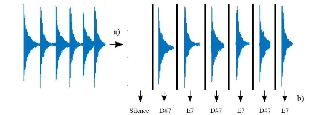
Automatic music transcription (AMT) consists in the same process done by a machine. According to Reis (Reis, 2012), the process of transcription is composed by two main tasks (see Figure 1.1): 1) extraction of the piano-roll notation and; 2) the conversion of the actual piano-roll into a score.

Figure 1.1 - The two main tasks of the transcription process. a) Extraction of the piano-roll notation taken from the music. b) Conversion of the piano-roll into a score.

It is worth mentioning, however, that AMT is mainly addressed as the extraction of the piano-roll notation. The conversion of the piano-roll into a score is, in fact, considered a different problem (Cemgil et al., 2006).

AMT can be decomposed into several sub-problems: pitch estimation, note onset/offset detection, loudness estimation and quantization, instrument recognition, extraction of rhythmic information and time quantization (Benetos et al., 2013). In this work, we mainly focus on one sub-problem called pitch estimation, or more specifically multi-pitch estimation. Pitch estimation consists in extracting the pitch of each musical note. In general, this transcription is done by splitting a musical piece into smaller chunks, called frames and then, afterwards, transcribe each one (see Figure 1.2).

(26)

Figure 1.2 - Common approach for pitch estimation process. a) Splitting the music in frames. b) Transcribing each frame.

On the other hand, multi-pitch estimation consists in the same process as pitch estimation but applied to polyphonic music. This process is much harder because there are much more factors that influence the quality of the signal, like, the overlapping of multiple notes and the characteristics of each instrument used. We can think of multi-pitch estimation as the process of discovering the ingredients of a given soup. Dominant ingredients can be easier to distinguish among all the flavors but secondary ones can be missed.

Many research works have been done focusing on the AMT problem. Some of these works are even in the market, as, it is the case of the AnthemScore (Lunaverus, n.d.). However, so far, none of these works has been able to reach, let alone surpass the human level in music transcription (Klapuri and Davy, 2007), (Sigtia et al., 2016a), (Bereket and Shi, 2017) and (Hawthorne et al., 2018), making this area still a very active research area.

1.1. Motivation

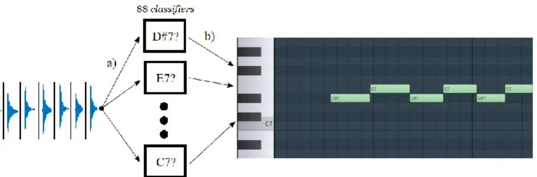
As mentioned above, AMT is the process1 of transcribing music automatically for which no suitable solution has been found so far. In general, this process is commonly though as a monolithic process where only one system is responsible for transcribing all the musical notes in a tune (see Figure 1.3). However, we can also think of it as a main process that contains multiple sub-processes, each one being responsible for detecting only one musical note (see Figure 1.4). This last point of view, is the one taken in this work. This approach that is also technically referred as divide to conquer technique is a common approach to be applied when dealing with hard problems. This is due to the fact that each sub-problem should be easier to solve. In this case, we refer to sub-processes as classifiers.

1_{When we refer to AMT as a process we are talking about the actual mechanical process of transcribing} music.

(27)

1.1. Motivation 3

Figure 1.3 - Monolithic process for transcribing musical notes. a) Insertion of frames into the AMT system. b) Notes that the AMT system can detect. c) Transcription result.

Figure 1.4 - Multiple classifiers, each one responsible for detecting a specific musical note. a) Insertion of the frames into each classifier. b) Transcription result from each classifier.

For this purpose, we built 88 classifiers, each one responsible for detecting a specific note. Please, keep in mind that, from now on we refer to this “new” approach as the one-classifier-per-note approach and the previous one (monolithic process) as the traditional approach. Some previous research works in AMT, have already adopted the one-classifier-per-note approach, as for example in (Marolt, 2004), (Poliner and Ellis, 2007), (Zalani and Mittal, 2014) and (Leite et al., 2016). However, in none of these works, it is possible to fully compare both approaches, due to the usage of a different technique to detect notes and/or due to a different dataset. As a result, a comparison between both approaches is presented in this work.

(28)

1.2. Goals and contributions

The main goal of this project is to present the one-classifier-per-note approach based on machine learning techniques. As mentioned above, this approach consists on having n classifiers, where each one is responsible for transcribing one note, instead of the traditional approach, of having one classifier responsible for transcribing all the notes. Additionally, it is also presented some post-processing steps to improve the final results.

The contributions of this project are as follows: • To update the current state-of-the-art.

• To present a comparison between the one-classifier-per-note approach and the traditional one.

• To present different types of post-processing steps.

• To collaborate by opening the source code of both scripts for creating the datasets and also for training the classifiers and the post-processing units.

• To publish a paper in the Portuguese Conference on Pattern Recognition.

1.3. Dissertation structure

The structure of the rest of this document is as follows:

• Chapter 2, Background – This chapter contains the concepts and terminologies needed to understand this work;

• Chapter 3, Related work – In this chapter a summary of works related to our project of the AMT field are described;

• Chapter 4, Proposed model – In this chapter our approach for the AMT problem is presented;

• Chapter 5, Preliminary experiments – In this chapter an overview of the preliminary experiments accomplished in order to achieve our final model are present;

• Chapter 6, Results – This chapter comprises the results achieved from our model as well as a comparison with other state-of-the-art works;

• Chapter 7, Conclusion and future work – In this chapter some final thoughts and conclusions are presented, as well as future work.

(29)

5

2. Background

The problem of automatic music transcription is a vast problem that combines different fields, from sound concepts and music theory to different types of digital processing methods. As a result, in this chapter we present the terminology and concepts that are necessary in order to understand the meaning of this work.

This chapter is divided into four main sections: general concepts, digital signal processing, multi-pitch estimation and aritificial neural networks.

In the general concepts section, an overview of the terminology and basic concepts is given. In the digital signal processing section, more advanced topics regarding signal processing are introduced. The multi-pitch estimation section compares single with multi pitch estimation. It also presents the main problems that can arise with pitch estimation problems. To finish, in the artificial neural networks section, an explanation about the artificial neural networks technique and its several variations are presented.

2.1. General concepts

Music is a form of art that is transmitted through sound. Thus, when dealing with music transcription, concepts regarding sound are also very important in order to achieve a good transcription.

In this section, basic concepts and terminologies such as what is referred as sound, the differences between digital and real-world sound, how a digital sound can have good quality, how a sound can be categorized and the main characteristics of the music, will be addressed.

2.1.1. Sound waves

We refer to sound as vibrations in some medium. Those vibrations, also called cycles, occur when the air is compressed (high pressure), rarefacted (low pressure) and finally returns to its original state. In general, human beings are able to hear vibrations from 20 to 20 000 times per second or, more technically, from 20 Hertz (Hz) to 20 Kilohertz (KHz), approximately. Any sound with a frequency bellow 20Hz is refered to as infrasound and above 20KHz as ultrasound.

In general, we visualize those vibrations in a digital format as, for example, in an oscillogram or in a computer program. These are represented as a function of time (see Figure 2.1), where

(30)

time is represented horizontally (x axis) and pressures values (amplitude) are represented vertically (y axis).

Figure 2.1 - Representation of the oscillations generated by a sound. The picture in the left side represents a sound generated mathematically and the picture in the right side shows a piano recording sound.

High levels of pressure (compression stage) are represented in the top part of the y axis, and low levels of pressure (rarefactor stage) in the bottom part of the y axis.

2.1.2. Digital audio recording

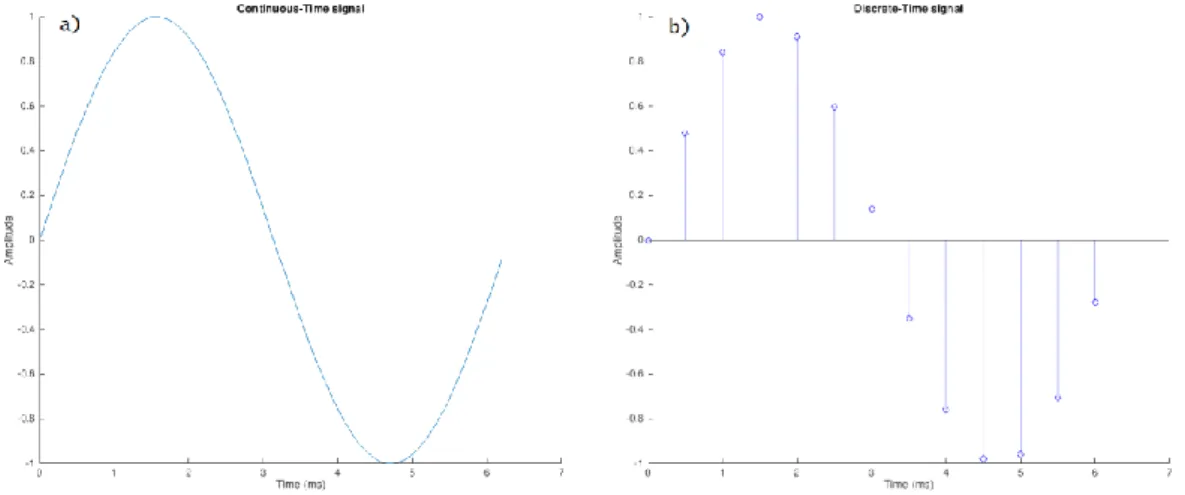
In the real world, the sound is continuous, or technically, it is referred as an analog signal. On the other side, in the digital world, the sound is discrete corresponding to an approximation of the reality (see Figure 2.2).

Figure 2.2 - Comparison of a continuous and a discrete signal. a) Continuous-time signal. b) Discrete-time signal.

Being the digital sound just an approximation, two main properties of it should be taken into account in order to have a good quality sound (close to the original sound): the sampling rate and the sampling resolution.

(31)

2.1. General concepts 7

Sampling rate

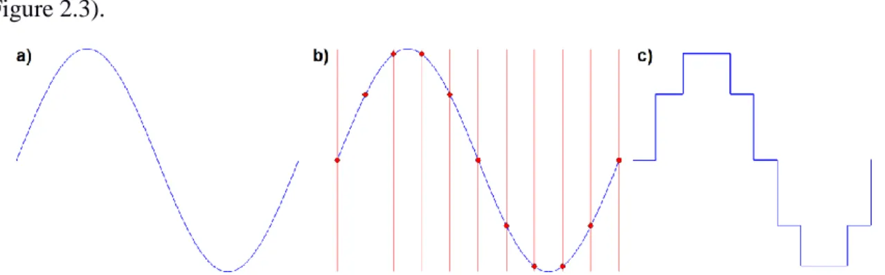
The sampling rate consists of the number of times an analog signal is measured (sampled) per second. The higher the number of samples per second, the more similar the digital audio is to the analog signal. If the sampling rate is too low, the digital signal may have not enough resolution and it can be considerably different from the corresponding analog version (see Figure 2.3).

Figure 2.3 - Low sampling rate problem. a) Sine wave. b) Low sampled sine wave. c) Resulting sampled version of the low sampled wave.

To avoid the problem above, the Nyquist theorem can be applied to determine the minimum sampling rate (see Figure 2.4). This theorem specifies that, the sampling rate must be at least twice the highest analog frequency component. Mathematically, this can be expressed as the following:

𝐹𝑠 ≥ 2 ∗ 𝐹𝑚𝑎𝑥, (24.1)

where Fs represents the sampling rate and Fmax represents the highest frequency contained in the analog signal.

Figure 2.4 - An example of a digital sound that follows the Nyquist theorem. a) High sampled sine wave. b) Resulting digital version of the sampled sine wave.

(32)

Sampling resolution

In the process of converting an analog signal to digital, the samples are stored as the closest amplitude value from the real one, within a set of possible values, technically refered to as levels. These levels depend on the bit depth used. The bit depth corresponds to the amount of bits available to characterize one sample (Figure 2.5). One bit of resolution contains two different values (0 or 1), a two bit resolution could store four different values (00, 01, 10, 11), a four bit could store 16 different values, a eight bit could store 256 different values, sixteen bit could store 65536 values, and so on. In the industry, 16-bit is the sampling resolution adopted for the Compact Disc (CD) to reproduce high quality music.

Figure 2.5 - Digital signal with a bit depth of 2. a) Sampled signal. b) Resulting digital signal with bit depth of 2.

2.1.3. Types of signal

Until now, we presented two types of signals, continuous-time signals and discrete-time signals. However, a signal can also be categorized into two categories: non-periodic or periodic.

A signal is denominated as periodic, when it repeats itself in another point of time (see Figure 2.6), while non-periodic the opposite scenario. Mathematically speaking, a periodic signal must follow the following equation:

𝑥̃(𝑡) = 𝑥̃(𝑡 + 𝑚𝑇), 𝑚 ∈ ℤ, (24.2)

where T is a real number. The lowest positive value of T where the equation above is still true, it is referred to as the period of the fundamental component and it is represented as 𝑇0.

(33)

2.1. General concepts 9

Figure 2.6 - Three examples of periodic signals.

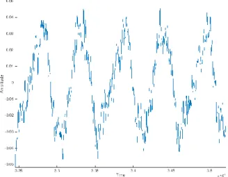
Also, a signal can be considered quasi-periodic when some discrete amplitude values are almost periodic (Figure 2.7), being the wave shape very similar in each repetition cycle but not exactly the same.

Figure 2.7 - Representation of a quasi-periodic signal. This sound was generated by a virtual piano software, playing the note E1.

2.1.4. Music characteristics

As mentioned previously, music is a form of art in which feelings, values and ideas are transmited through sound. Each played musical note has four fundamental characteristics: dynamics, duration, timbre and pitch.

Dynamics or note velocity in Musical Instrument Digital Interface (MIDI) terminology (Association, 1999) is the characteristic that refers to the volume or loudness of a sound. The most common dynamic indications are known as pianissimo (very soft), piano (soft), forte (loud) or fortissimo (very loud).

(34)

Duration is the time interval during which the musical note lasts. The moments in which the sound starts and ends are designated by onset and offset, respectively.

Timbre represents the type of the sound. It is the shape of the sound wave. This characteristic is what makes us differentiate a piano sound from a person singing.

Pitch is the tonal height of a sound. It represents how low or high a note sounds and it is closely related to the frequency: the physical property. In addition to that, it is the characteristic responsible for distinguishing different notes of the same instrument.

2.2. Digital signal processing

Digital signal processing (DSP), a sub-field of signal processing, consists in the application of computational methods on digital signals in order to extract features, which are used in analysis, classification, recognition or transformation problems.

The file format, Joint Photographic Expercts Group (JPEG), is a good example of where these techniques are applied in order to compress the size of images (Bako, 2004). Additionally, DSP techniques are commonly applied in order to estimate the velocity or the distance travelled of an object, by detecting the shift on the frequency signal received from a radar (Giordano, 2009).

In this work, DSP techniques are also applied in order to reach our goal, that is, transcribe piano music. Thus, basic terminologies like the frequency unit and more advanced ones such as how a signal can be decomposed into frequencies and a deeper understanding of some DSP methods, with a special focus to the set of methods from the family of the Fourier Transform, are introduced. At the end, problems and possible solutions, if any, regarding these methods will also be presented.

2.2.1. Fourier analysis

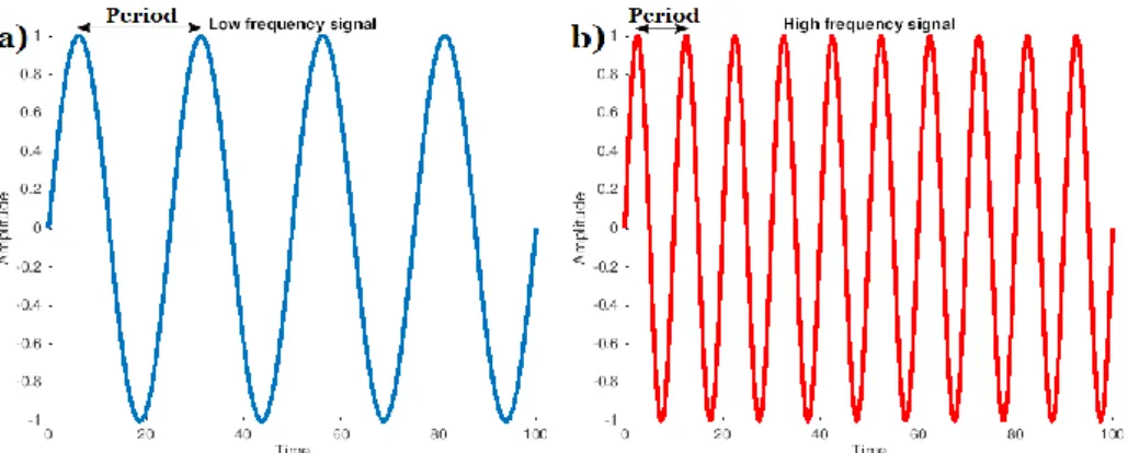
As stated before, sound consists in cycles (back and forth) in a medium. The number of cycles per unit of time of a sound wave is named as frequency. A sound with a high frequency contains a large number of cycles and small wavelength (period). On the contrary, a sound with low frequency has less number of cycles and a larger wavelength (Figure 2.8).

(35)

2.2. Digital signal processing 11

Figure 2.8 - Low and high frequency representation. a) Represents a low frequency sound wave. b) Represents a high frequency sound wave.

Jean-Baptiste Joseph Fourier was the first to have the vision that any continuous function could be represented as an infinite sum of simple sinusoids. That was later demonstrated to be true (Oppenheim et al., 1997). These sinusoids are simple waves mathematically represented by sines and cosines or complex exponentials. Due to the properties of those sound waves (sinusoids), it is possible to recover their frequency. It is important to point out that in a polyphonic signal, the sinusoid with the lowest frequency from all the sinusoids is considered as the fundamental frequency (F0). The F0, in music, is the main frequency closely related to the perceived musical pitch. Remember that the musical pitch is what makes us able to distinguish between different notes.

The process of decomposing a periodic signal into the sum of harmonics is known as Fourier analysis (Figure 2.9 a). The opposite process, of rebuilding a periodic function from those simple waves is denominated as Fourier synthesis (Figure 2.9 b).

Figure 2.9 - Example of both the Fourier analysis and the Fourier synthesis processes. a) Decomposing signal into simple waves (Fourier analysis). b) Rebuilding a signal with simple waves (Fourier synthesis).

There are several known techniques to decompose a signal, depending on its characteristics: discrete or continuous and periodic or non-periodic. Within the scope of this work, the most important techniques are the Fourier Series and the Discrete Fourier Transform (DFT).

(36)

Fourier Series can be applied to periodic and continous signals, and the Discrete Fourier Transform can be applied to quasi-periodic and discrete signals. As mentioned before, digital sound signals are discrete, hence it is important to keep in mind that only the DFT technique can be applied in this work.

Fourier series

Mathematically, the process of Fourier synthesis where the sum of infinite harmonics occurs, can be represented as follows:

𝑥̃ = ∑ 𝑎𝑘𝑒𝑗𝑘ω0𝑡, 𝑘 ∈ +∞

𝑘=−∞

ℤ, (24.3)

where ω₀ = 2𝜋𝐹0 = 2𝜋

𝑇0. An important point to consider in the Fourier series representation

is that the harmonics forms an orthonormal set. This is relevant because the resulting integral and product will be zero. Hence, the process of Fourier analysis can be efficiently computed as follows: 𝑎_𝑘 = 1 𝑇₀∫ 𝑥̃(𝑡)𝑒 −𝑗𝑘ω0𝑡 𝑇0 𝑑𝑡. (24.4)

By readjusting the previous equation, of the fourier synthesis process, we have:

𝑥̃(𝑡) = 𝑎₀ + ∑(𝑎_𝑘𝑒𝑗𝑘ω0𝑡_{+ 𝑎} −𝑘𝑒−𝑗𝑘ω0𝑡) = +∞ 𝑘=1 𝑎₀+ ∑(𝑎_𝑘𝑒𝑗𝑘ω0𝑡_{+ 𝑎} 𝑘 ∗_𝑒−𝑗𝑘ω0𝑡₎ +∞ 𝑘=1 , (24.5)

where 𝑎_𝑘∗ = 𝑎_−𝑘. Finally, by considering 𝑎_𝑘 in the polar form as 𝑎_𝑘 = 𝐴𝑘

2 𝑒

𝑗𝜙𝑘_{, we have a} trigonometric equation as follows:

𝑥̃(𝑡) = 𝑎0+ ∑ 𝐴𝑘cos(𝑘ω0𝑡 + 𝜙𝑘) +∞

𝑘=1

. (24.6)

This resulting equation (Equation 24.6) is frequently used for representing periodic signals in the Fourier series. If a sound can be represented using this last equation, it is called a harmonic sound. Since quasi-periodic signals have slightly different frequencies per each wave cycle, they are often cited as partials. Hence, an approximation of quasi-periodic signals is commonly used, with a finite number of harmonic components H:

(37)

2.2. Digital signal processing 13 𝑥̃(𝑡) ≈ 𝑎0+ ∑ 𝐴𝑘cos(𝑘ω0𝑡 + 𝜙𝑘) . 𝐻 𝑘=1 (24.7) Fourier Transform

Fourier transform and all its variations are techniques used to convert signals from the time domain (time-amplitude) into the frequency domain. These methods are commonly used by AMT systems because, as mentioned previouslly, pitch is a characteristic from music that gives us the possibility to distinguish notes from the same instrument and this characteristic is closely related to the frequency, making these methods highly relevant for the AMT problem.

The Fourier transform decomposes the signal into a sum of simple waves (fourier analysis) resulting in the frequencies of the signal. This technique is used for periodic continuous signals with infinite length as follows:

𝐹𝑇_𝑥̃(𝑓) = 𝑋̃(𝑓) = ∫ 𝑥̃(𝑡)𝑒−𝑗2𝜋𝑓𝑡_𝑑𝑡. +∞

−∞

(24.8)

Discrete Fourier Transform

As mentioned above, the Fourier Transform technique can only be applied to periodic continuous signals. However, a digital signal is discrete. Hence, another technique called Discrete Fourier Transform (DFT) is applied. The DFT can be calculated as follows:

𝐷𝐹𝑇_𝑥̃[𝑘] = 𝑋̃[𝑘] = ∑ 𝑥̃[𝑛] +∞

𝑛=−∞

𝑒−𝑗2𝜋𝑘𝑛_, _(24.9)

where k is the spectral bin corresponding to each frequency. In Equation 24.9, infinite discrete signals are targeted. However, infinite signals create computational problems. Thus, Equation 24.10 is defined to tackle this problem:

𝐷𝐹𝑇_𝑥̃[𝑘] = 𝑋̃[𝑘] = ∑ 𝑥̃[𝑛] 𝑁−1

𝑛=0

𝑒−𝑗2𝜋𝑁𝑘𝑛_{, 𝑘 = 0, … , 𝑁 − 1,} (24.10)

where N represents the length of the waveform (number of samples).

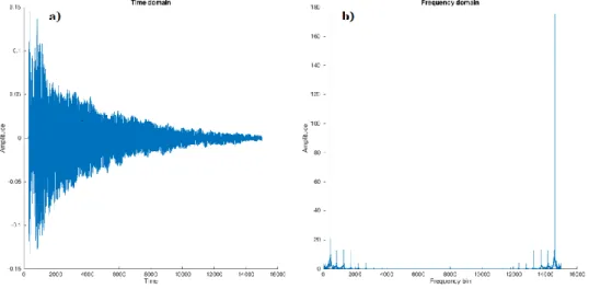
There are two main points that are necessary to be clarified here before we proceed. The first one, is that according to Shannon (1998), only the first half of the samples (until the Nyquist frequency) are relevant because the second half is just a mirror of the first half (Figure 2.10). The second point is that each value on the frequency domain represents a spectral bin, more

(38)

specifically, it represents a range of frequencies and not just one frequency. For example, if a signal has 4096 samples and its sampling rate is 44100 Hz, each bin is linearly separated by ∆𝑓 = 𝐹𝑠

𝑁 = 44100

4096 ≅ 10.77𝐻𝑧. Thus, each spectral bin k will contain a range of frequencies between 𝑓𝑘 = 𝑘 ∗ 10.77𝐻𝑧 ± 10.77𝐻𝑧. As a result, some piano notes correspond to the same spectral bin, making the process of detecting notes harder.

Figure 2.10 - A comparison of the same sound in two different domains. a) Sound in the time domain. b) Sound in the frequency domain.

Fast Fourier Transform

DFT is a common technique used for periodic discrete signals. However, this technique can be computationally expensive for real time applications, such as AMT systems. Thus, in order to fulfill this necessity, another technique called fast Fourier Transform (FFT) is used. This is the DSP technique applied in our work.

FFT is a fast algorithm which applies efficiently the DFT in a signal that contains a structured number of samples such as the power of two. This technique reduces the number of operations from 𝑂(𝑁2_{), where N represents the number of samples, to 𝑂(𝑁 ∗ 𝑙𝑜𝑔}

2𝑁) (Cooley et al., 1967).

(39)

2.2.2. Spectral leakage

The DFT and its variations assume that a signal is periodic. However, if the number of samples does not match with the whole number of periods, discontinuities will occur, leading to a distorted frequency representation. This event, known as spectral leakage, leads to frequencies being leaked or spread across adjacent frequency bins (see Figure 2.11).

Figure 2.11 - Representation of the spectral leakage event. a) Signal with 30 samples, which corresponds to the whole number of periods. b) Signal with 25 samples causing the spectral leakage event, that can be viewed in the zoomed frequency spectrum on the right.

2.2.3. Windowing

In order to minimize the spectral leakage, a technique called windowing can be used, where the input signal is, firstly, multiplied by a smooth window, and only then the DFT is calculated. Resulting in a smoother frequency signal. There are several types of windows: rectangular, triangular, Hanning, Hamming, Blackman and Blackman-Harris. All of them have their pros and cons. A comparison can be found in (Harris, 1978). This technique can be calculated as follows:

(40)

𝑌𝑘 = ∑ 𝑎𝑛𝑥̃𝑛𝑊𝑁𝑛𝑘, 𝑊 = 𝑒−𝑗2𝜋, 𝑁−1

𝑛=0

(24.11)

where 𝑎𝑛 is the the type of window. 2.2.4. Missing fundamentals

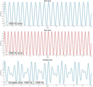
As mentioned previously, pitch is a characteristic that can be found in music and is closely related to a physical property called frequency. However, the pitch characteristic is also related to the spectral content and the loudness of a sound. This means that the frequency is not considered as a clear representation of the pitch characteristic. Therefore, when analysing the frequency of complex sounds, a phenomenum called missing fundamental commonly arises. For instance, when an audio signal is composed of two pure tones, one of them with 1000 Hz and another one with 1300 Hz, an additional tone would be perceived at 300 Hz (Figure 2.12).

Figure 2.12 - An example of missing fundamental resulting at 300 Hz. a) 1000 Hz pure tone. b) 1300 Hz pure tone. c) complex tone: 1000 Hz + 1300 Hz pure tones.

(41)

2.2.5. Pitch vs Fundamental frequency

Regarding the frequency of a given sound, a common error is made: What is the frequency of the piano MIDI note number 55?

The sentence above is not completely correct because a piano note (like most of the sounds) do not contain a single frequency, but instead it is composed by several frequencies (harmonics). A better question would be the following one:

What is the fundamental frequency of the piano MIDI note number 55?

The fundamental frequency (F0), as mentioned previously, is the lowest frequency on an harmonic series and is the essential one in order to distinguish a pitch in a given signal. For instance, if a piano note sound has an F0 around 260Hz, our brain should be able to map it as a C4 pitch (see Table 2.1).

Table 2.1 - Corresponding frequency of each pitch, from C0 to B8.

Note

Octave

0 1 2 3 4 5 6 7 8 C 16 33 65 131 262 523 1047 2093 4186 C# 17 35 69 139 278 554 1109 2218 4435 D 18 37 73 147 294 587 1175 2349 4699 D# 20 39 78 156 311 622 1245 2489 4978 E 21 41 82 165 330 659 1319 2637 5274 F 22 44 87 175 349 699 1397 2794 5588 F# 23 46 93 185 370 740 1475 2960 5920 G 25 49 98 196 392 784 1568 3136 6272 G# 26 52 104 208 415 831 1661 3322 6645 A 28 55 110 220 440 880 1760 3520 7040 A# 29 58 117 233 466 932 1865 3729 7459 B 31 62 124 247 494 988 1976 3951 7902

(42)

In the field of AMT two different terms are commonly confused: F0 estimation and pitch estimation. F0 estimation consists in the extraction of the exact frequency components of a signal and then match them to the pitches of the notes. The second process, pitch estimation, consists on determining the pitch from a given signal even without knowing exactly the F0 of the sound. This last process is the one applied in this dissertation.

2.3. Multi-pitch estimation

Multi-pitch estimation algorithms commonly assume that there can be two or more harmonic sources in the same short-time signal. According to Yeh et al. (2010), a signal can be expressed as a sum of harmonic signals plus the residual part:

𝑦[𝑛] = ∑ 𝑦𝑚[𝑛] + 𝑧[𝑛] 𝑀

𝑚=1

, 𝑀 > 0 with 𝑦𝑚[𝑛] ≈ 𝑦𝑚[𝑛 + 𝑁𝑚], (24.12)

where n represents the discrete time index, M is the number of harmonic signals, 𝑦_𝑚[𝑛] the quasi-periodic part of the mth source, 𝑁_𝑚 the period of the mth source and z[n] the residual part.

This combination of harmonic sources makes the process of estimating the pitches even harder. In a monophonic signal the notes are played separately and therefore, it does not suffer any type of distortion from other harmonic sources, which is not the case in a polyphonic signal (see Figure 2.13 and Figure 2.14).

Figure 2.13 - Representation of a monophonic signal, where each note (C#, C, D# and F#) are played separately.

Figure 2.14 - Representation of a polyphonic signal. a) A chord of 2 notes (C# and C), been played simultaneously. b) A chord of 4 notes (C#, C, D# and F#) played simultaneously.

As it is possible to notice, the more harmonic sources a signal has, the harder the process of estimating the pitches.

(43)

2.3. Multi-pitch estimation 19

In addition to that, other types of problems, can also occur, such as the distortion of a signal because of its residual components. The residual components are all the components that cannot be explained by simple waves (sinusoids), as for example the background noise, non-harmonic partials or spurious components.

In the following sections, several common problems regarding the multi-pitch estimation problem are presented.

2.3.1. Overlapping partials

As mentioned above, in polyphonic signals, different sources may overlap or interfere with each other. Those different sources can be considered in harmony if their fundamental frequencies (𝐹𝑎 and 𝐹𝑏) can be represented as follows:

𝐹_𝑎 = 𝑚

𝑛 𝐹𝑏, 𝑛, 𝑚 ∈ ℕ, (24.13)

in which every 𝑛𝑡ℎ partial of the source a overlaps every 𝑚𝑡ℎ partial of source b, as proved by Klapuri in (Klapuri, 1998). This augments the probability of partial collisions. Another issue demonstrated in (Yeh, 2008) occurs when the F0 of a note is multiple of another note’s F0. In this case, the higher note can hide the lower one.

Interference and overlaping of different sources can disturb a signal in several ways, as its frequencies, amplitudes and phases. For instance, when two sources are superposed, the resulting sound wave would be a sum of those two sources. On the contrary, when there is a harmonic overlap, the resulting wave would have two simple harmonic motions with the same frequency but with different amplitude and phases.

There are several works in which the authors tried to detect those overlaping partials, which in the case of being successful could help in the process of multi-pitch estimation. In (Parsons, 1976) the author tried to detect those overlapping components based on three tests: spectral peak symmetry, distance and well-behaved phase. However, even with only two different sources, that is actually a very restrictive number of sources, the results were not good. Later on, several authors (Viste and Evangelista, 2002), (Virtanen, 2003), (Every and Szymanski, 2004) and (Yeh and Roebel, 2009) tried to address the problem by knowing in advance how many different sources existed in a given signal but unfortunatelly the results were poor. Thus, this problem remains a challenge.

(44)

2.3.2. Spectral characteristics

In a musical piece, it is common that several types of instruments are played simultaneously. This adds even more complexity to the transcription problem.

In the following three sub-sections, different types of instrument characteristics are present, such as: the spectral envelope, inharmonic partials and spurious components.

Spectral envelope

We refer to the spectral envelope, as the contour of the prominent peaks of a given signal, in which most of them are partials (see Figure 2.15). Each musical instrument has a different spectral envelope, as for example pianos and trumpets. Even instruments of the same family, as for instance two pianos, have slightly different spectral envelopes. According to Jensen (Jensen, 1999), Loureiro et al. (Loureiro et al., 2004) and Burred et al. (Burred et al., 2006), still an universal model that generalizes different types of instruments needs to be developed.

Figure 2.15 - An example of the spectral envelope. Inharmonic partials

In an ideal harmonic sound, the frequencies of the harmonics are integer multiples of the fundamental frequency. However, in real musical instruments this does not occur. Those deviated harmonics (from the ideal F0) are called inharmonic partials, and it is a common phenomenum in string instruments.

(45)

2.3. Multi-pitch estimation 21

Spurious components

Another type of influent characteristic that can be also observed in string instruments is the one called phantom partials. According to Conklin (Conklin, 1999), these phantom partials, in string instruments are related to the tension variation on the plucked strings, and are close to the frequencies of the normal partials. Nevertheless, recent works (Moore et al., 2017) and (Moore et al., 2018) also suggest that non-string components, like the mechanical parts or the wooden components of a piano, could also contribute to the appearance of those phantom partials. These kind of partials are sometimes fairly dominant compared to the normal partials, which in turn can lead to a bad transcription.

2.3.3. Transients

In music, it is quite common, specially in some types of musical pieces, that the notes are played roughly, resulting in abrupt variations in the sound signal. According to Rodet and Jaillet (Rodet and Jaillet, 2001), these fast variations are denominated as transients. The transients usually refer to note onsets (fast attacks) or to note offsets (fast releases). Due to those abrupt variations and also that most of the variations have high levels of energy, the sound signal will contain several spurious components, making the process of estimating the pitch in those areas very hard. Recent research works tend to consider the transient as a specific signal component, where it is detected by either a parametric approach (Daudet, 2004) and (Molla and Torrésani, 2004), or a non-parametric approach (Rodet and Jaillet, 2001), (̈obel, 2003) and (Bello et al., 2005).

2.3.4. Reverberation

When a note is played and then released, the sound produced does not disappear suddenly. It usually takes time in order to be not earable anymore. This process, the prolongation of a preceding sound is called reverberation. Thus, a recorded signal can be considered as a mixture of multiple sounds, which are direct sounds, reflected sounds and reverberated sounds. According to Yeh et al. (Yeh et al., 2006), Beauchamp et al. (Beauchamp et al., 1992) and Baskind et al. (2012), depending on the recording environment, a monophonic sound can also become a polyphonic sound, because the reverberated and reflected sounds add complexity to the analysis of the recorded signal.

(46)

2.4. Artificial neural networks

Artifical neural networks (ANNs) or simply neural networks are an artificial intelligence (AI) technique based on biological brains. This technique has been used successfully in many complex problems, such as: autonomous vehicles (Bojarski et al., 2016), autonomous farm (Pearlstein et al., 2016), (Luo et al., 2010) and (Stentz et al., 2002), anomaly detection in internet traffic (Pradhan et al., 2012), cancer detection in medical images (Singh et al., 2015) and also music transcription (Sigtia et al., 2016a) and (Kelz et al., 2016). This is one of the reasons whereby we have applied ANNs in this work, because they are good at tackling difficult problems and, apart from that, it’s a technique already applied in the AMT problem, and thus, a more closer comparison with other works can be made.

This section is divided into five topics: neuron model, ANN architecture, learning method, types of activation functions and types of ANNs. Initially, a comparison between the biological neuron and an artificial neuron is presented. Then, an overview of the main components of an ANN is introduced. Continuing, an explanation of how the ANNs learn is presented. To conclude, a deeper explanation regarding activation functions, following by an introduction of several types of ANNs are presented.

2.4.1. Neuron model

As mentioned above, ANNs were inspired by biological brains. The human brain has roughly 86 ∗ 109 of connected elements, called neurons. Each neuron, is composed by three main components (see Figure 2.16, bellow): the dentrites, the cell body and the axon. The dentrites are tree-like connections that receive and transport incoming signals to the cell body. Hence, the cell body is the component responsible for processing the incoming signals, by summing and thresholding. However, sometimes, the dentrites also process those informations before it arrives to the cell body. The last main component, the axon, is in charge of transporting and transmiting the output signal from the cell to other neurons. The transmition, is done in the edge of the axon in a zone called synapse. Synapses transform the electrical signal into a chemical one and, then, send it to the dentrites of other neurons.

(47)

2.4. Artificial neural networks 23

Figure 2.16 - Representation of a biological neuron. Adapted from (Pixabay).

On the other side, a neuron of an ANN is composed by three main elements (see Figure 2.17, bellow): the connection weights or simply the weights, a bias weight and an activation/transfer function. Each connection weight, represents the relevance of the connection that the neuron is attached to. The bias weight, or just bias, is a special weight attached to a special connection with a constant input that helps the artificial neuron to adapt itself better to the data received. The activation function is a linear or non-linear function that is used in order to modulate the output result. It receives as input the weighted sum of the inputs.

Figure 2.17 - Representation of an artificial neuron. p represents the inputs vector, w the weights vector, b the bias, n the weighted sum of the inputs, f the activation function and a the output result of the neuron.

If we relate the artificial neuron with the biological neuron seen above, we can consider each weight (𝑤_𝑥) as the strength of the respective synapse, the summation and the activation function (f) as the cell body and the output result of the neuron (a) as the signal on the axon. Mathematically, the output result of a multiple-input neuron can be calculated as follows:

𝑎 = 𝑓(𝒘𝒑 + 𝑏), (24.14)

where w represents a vector of weights and p the inputs vector, b the bias and f the activation function. For a given w and p of size n, the calculus would be as follows:

(48)

2.4.2. ANN architecture

In general, a single artificial neuron is not enough to extract meaning from the data itself, even if that neuron has multiple inputs. It is more common to use a group of neurons, called layer, which works in a parallel way. In an ANN, there are three types of layers (see Figure 2.18): the input layer, that is basically the input data; the hidden layer, which are all the layers placed between the input and the output layer and where most of the extraction of meaning is done; finally, there is the output layer, which is the last layer of the network and which in turn is responsible to output a final result based on the features extracted by the hidden layers.

Figure 2.18 - Representation of an ANN with a single hidden layer, where it is possible to distinguish between the three different types of layers.

During several years, ANNs had no hidden layers. The reason of that was because no one knew how to “teach” an ANN with multiple layers. Only after the proof of work in (Rumelhart et al., 1986), of an algorithm called backpropagation, was when ANNs started to include hidden layers (see Figure 2.19). In general, ANNs with multiple hidden layers perform much better than a single layer neural network. Nevertheless, the more layers an ANN has, the more parameters the ANN needs to learn which in turn increases the difficulty of the learning/training process. Thus, for each problem a study of different number of layers and neurons is commonly done.

(49)

2.4.3. Learning method

The way an ANN learns, also called training process, can be divided into two main steps: forward propagation and backpropagation. The forward propagation is the step where the neural network outputs a result from the given input data. This result is calculated by applying equation 24.14 (see above), to each neuron, starting from the first layers up to the last one, until an output result from the network is given. Note that all the outputs from a layer are used as input of the following one (see Figure 2.19, above).

This final output of the network, technically called prediction, is then used for the next step, called backpropagation. In the backpropagation step, a readjustment of the weights of the network is done, according to how close the prediction is to the reality (label). The idea consists in doing changes to the weights proportional to the negative derivative of the error. This type of learning, where a reality is known is called supervised learning. Nevertheless, there are other types of learning, like unsupervised learning, where no label is known in advance and the algorithm learns by identifying commonalities from the data, or even reinforcement learning, where the algorithm learns by receiving rewards from the actions (predictions) taken in a given enviroment, like a game.

Backpropagation can be divided in two main steps: the calculation of the error and the update of the weights. In the process of calculating the error, an error is calculated for each layer, starting from the output layer and then backpropagating it down to the input layer, layer by layer. In the end, each neuron has an error associated. These errors are then used to adjust the weights. The adjustement of each weight is called gradient.

2.4.4. Types of activation functions

As mentioned in the beginning of this chapter, ANNs are applied in almost any kind of problem. The peculiarity of this technique, is that a suitable solution can be found for almost any type of non-linear problem (see Figure 2.20). However, this peculiarity, as we mentioned, it is only possible if a non-linear activation function is applied. Thus, most of the time a non-linear activation function is used.

(50)

Figure 2.20 - Example of a linear and a non-linear problem. a) linear problem where a simple straight line is able to separate the circles from the squares. b) non-linear problem where a straight line is not able to separate the circles from the squares, thus, as an alternative, a circular line is applied.

There are several types of non-linear activation functions, like: the sigmoid, the hyperbolic tangent (tanh), the softmax, the softplus (Dugas et al., 2000), the swish (Ramachandran et al., 2017) and the rectified linear units (relu) and also its variations like the leaky relu and the scaled exponential linear unit (selu) (Klambauer et al., 2017). Commonly, activation functions like the softplus, rectified linear units or the swish are used for the hidden layers. On the other side, the sigmoid, the softmax and the tanh are used in the output layer, as can be seen in the following works: (Nair and Hinton, 2010), (Zeiler et al., 2013), (Senior and Lei, 2014), (He et al., 2015), (Ioffe and Szegedy, 2015) and (Ramachandran et al., 2017). There are several reasons for this common approach, like the computation time (relu and most of its variations), ideal output for classification (sigmoid, tanh or softmax) and problems like the vanishing gradient2 or not being zero centered3 (these last two problems can make the training process longer). In the following figures, a representation of all the previously mentioned activation functions, except the softmax (due to being a multi-class4 activation function), are presented. Nevertheless, according to Rennie the softmax is convex (Rennie, 2005).

2_{The vanishing problem consists on small updates of the weights due to an almost zeroed derivative.} 3_{A not zero centered function can introduce undesirable zig-zagging in the gradient updates (all positive} or all negative gradients).

4_{A multi-class activation function is a function that has two or more possible outputs. However, it is} more commonly applied in problems that have three or more.

(51)

Figure 2.21 - Representation of several activation functions.

2.4.5. Types of neural networks

One of the drawbacks of the artificial neural networks technique is that it is computationally expensive. However, due to the computer power being growing almost exponentially and its price being decreasing, this drawback has almost vanished, whereby today its one of the most popular techniques to be applied in several types of problems. As a result, several types of artificial neural networks have been created: the traditional feedforward neural network, simply refered to ANN, recurrent neural networks (RNNs) and convolutional neural networks (CNNs), to name just a few.

An ANN is a type of neural network where the information of the input data moves only in one direction and where time is not taken into account. On the other side, an RNN, is an ANN that tries to take advantage of sequential information from the input data. This can be a major advantage when dealing with problems such as language translation or even music transcription. However, this type of network can be very hard to train. Another type of ANNs that have been responsible for major breakthroughs, specially in problems such as vision, are CNNs. This type of technique has been developed mainly because simple ANNs perform poorly when applied to problems with images and also because the input data of an ANN must have a strict size, which is not usual, in the case of images. However, CNNs also use

(52)

simple ANNs, but they are only applied after the input data is “parsed/filtered” by convolutional and (commonly) pooling layers. We can think of both these layers as a way of extracting the main features of an image. In addition to that, also the pooling layer is responsible for transforming the input data into a strict size.

2.5. Summary

This chapter presented several important topics of the dissertation. The topics range from general basics such as sound and music characteristics to more specific concepts such as deeper analysis of digital signal processing. The chapter also touched on artificial neural networks.

Remember that, most AMT systems commonly apply methods such as the FFT, referred above, to a sound signal to be easier in detecting pitches on it. However, these methods have their own set of problems, namely: missing fundamentals and spectral leakage. Regarding spectral leakage, a possible solution called windowing could be applied in order to attenuate the problem. For missing fundamentals, to the best of our knowledge, currently, there is no known solution. Another important point is that, ANNs are good problem-solvers for almost any type of complex problem, including automatic music transcription. As a result, we have applied in this work the FFT and the ANN technique.

In the following chapter, a review of other research works related to single and multi estimation problems are presented, in order to understand how other authors tackled them.

(53)

29

3. Related work

This chapter reviews related works of the AMT field. The review has three main sections: 1) general overview; 2) artificial neural networks and 3) genetic algorithms.

3.1. General overview

The problem of transcribing monophonic music automatically can be considered solved. However, automatic transcription of polyphonic music is still being researched.

Since the first polyphonic music transcription system (Moorer, 1975), several posterior related works have been presented. These works have originated the appearance of several different approaches to the AMT problem. According to Yeh (Yeh, 2008), those approaches can be classified into two groups: iterative estimation approaches and joint estimation approaches.

3.1.1. Iterative estimation

An iterative estimation approach consists in finding the most predominant-F0 estimation, apply the respective cancelation or surpression technique and repeat this process until the termination condition is met. This approach assumes that per each iteration a dominant source exists. When this assumption is not met, the iteration process can lead to an accumulation of errors.

There are two types of cancelation techniques, direct cancellation and cancellation by spectral models.

Direct cancellation

Direct cancellation applies a single-F0 estimation algorithm to extract the predominant-F0 and then removes all harmonics of the extracted source from the observed input signal. This technique assumes that the complete removal of the dominant source does not affect the following estimations. The term “direct” cancellation denotes that the source interaction, as for example, overlapping partials, are not taken into account.

In (Parsons, 1976) the author applied the Schoroeder’s histogram in order to extract the predominant-F0s in a two-speaker separation problem. After the first F0 estimation, the spectral peaks corresponding to its harmonics were excluded before the calculation of the next histogram. In (Lea, 1992) the author used a method that iteratively extracts the predominant peak in the summary autocorrelation as an F0 and cancels the estimate in the

(54)

autocorrelation array. In 1993, in the work (Cheveigné, 1993), the author proposed a time-domain cancellation model where both iterative and joint approaches were studied. The iterative cancellation approach was responsible for estimating the predominant F0 by average magnitude difference function and cancel it by comb filtering. Direct cancellation was also used on the spectral domain. In (Ortiz-Berenguer et al., 2005), the authors used spectral patterns trained from previously recorded piano sounds to perform harmonic matching. The predominant-F0s found were removed iterativelly by means of binary masks around the matched harmonics in the observed spectrum.

Cancellation by spectral models

In (Klapuri, 2003) the author introduced an algorithm based on harmonicity and spectral smoothness. In the preprocessing stage a RASTA-like technique (Hermansky and Morgan, 1994) a logarithmic frequency scale is used, to compress the spectral magnitudes and remove the additive noise. The resulting spectrum is then splitted into multiple frequency bands. F0 weights are calculated on each band by normalizing the sum of their partial amplitudes and by taking into account the inharmonicity. The predominant weights, from those resulting F0 weights, are then smoothed using an algorithm described in (Klapuri, 2001) and finally subtracted from the signal spectrum to avoid its corruption after several iterations of direct cancellation. This way, the overlapping partials still contain energy for the following sources. This method, which is denominated by bandwise smooth model, uses the moving average over the amplitudes within one octave band in order to smooth the envelope of an extracted source. This process is repeated until the maximum weight related to the signal-to-noise ratio is lower than a certain threshold.

Later on, in (Klapuri, 2005) a perceptually motivated multiple-F0 estimation method is presented. Initially, subband signals were compressed and an half-wave rectifier was applied. Harmonic matching is then applied on the summary spectrum. This way, the predominant F0 is extracted. Then, a 1/k smooth5 is used to smoothen the predominant source

while retaining energy of higher partials for the next iteration. Later on, in (Klapuri, 2006), the author proposed a spectral model, similar to the previous mentioned 1/k smooth model, which attempts to generalize a variety of musical instrument sounds.

In (Santoro and Cheng, 2009) the authors presented an algorithm based on Klapuri’s work, for multiple F0 estimation using the modified discrete cosine transform domain.