Influence of physical modifications of the wing on an aircraft’s fuel consumption

UNIVERSIDADE DA BEIRA INTERIOR

Faculdade de Engenharia

Influence of physical modifications of the wing on

an aircraft’s fuel consumption

Numerical Analysis

João Jacinto

Dissertação para obtenção do Grau de Mestre em

Engenharia Aeronáutica

(ciclo de estudos integrado)

Orientador: Prof. Doutor Pedro Gamboa

Acknowledgements

First of all, I would like to thank my parents and sister for the support they gave me through all my life, this one is for them.

To my girlfriend for all the patience and comprehension.

To all my teachers, especially my advisor Professor Pedro Gamboa, PhD, for the guidance they provided through all these years.

To all my friends. Your companionship made these five years a lot easier for me to overcome. And last, but not least, to Eng. Hugo Raposeiro for all the information and help provided.

Resumo

O objectivo deste trabalho é, através da aplicação de métodos de cálculo encontrados nas obras referidas e das fórmulas que lhe são intrínsecas, obter uma forma de calcular e interpretar numericamente quais as influências de cada alteração física da asa no consumo de uma aeronave durante um voo típico de cruzeiro, comparando-o com o consumo de uma aeronave de base.

Em termos de alterações físicas da asa da aeronave, foram feitas variações de Razão de Aspecto, de Área Projectada, Afilamento e Ângulo de Enflechamento. Duas outras alterações foram efectuadas, o Bypass Ratio dos motores e a velocidade de cruzeiro. Estas não são relacionadas directamente com a asa, mas foram implementadas de modo a dar outras aproximações à questão.

Chega-se à conclusão que uma razão de bypass e uma razão de aspecto maiores, aliados a uma área de asa, afilamento e enflechamento mais reduzidos levam a um consumo menor, originando uma aeronave óptima para cada uma das cinco velocidades de cruzeiro.

Cada um dos pontos óptimos foi então sujeito a um estudo de implementação de compósitos avançados nas suas estruturas principais, demonstrando que as partes que mais influenciam o peso vazio da aeronave e o seu consumo de combustível são a fuselagem, as asas e os motores.

Palavras-chave

Green Aircraft; Consumo de combustível em voos comerciais; Uso de compósitos avançados; Influência da asa no consumo; Cruzeiro de curto – médio alcance.

Abstract

The goal of this assignment is to obtain a way to calculate and to interpret numerically the influences of each physical transformation of the wing on an aircraft’s fuel consumption in a typical cruise mission, comparing it to a reference aircraft by applying calculation methods found in the works of Daniel P. Raymer, Denis Howe, among others.

Regarding the physical alterations made in the wing, there was a variation of the Aspect Ratio, Projected Area, Taper Ratio and Sweep. Two other aspects were also altered, the engines Bypass Ratio and the cruise speed. Although those are not wing characteristics, they were implemented to provide more data, making the assignment more complete.

The conclusion achieved was the fact that an increase in the bypass ratio and aspect ratio, associated with a decrease in wing surface, sweep and taper ratio led to a lower required fuel weight, originating an optimal aircraft for each of the five cruise speeds.

Each of these points was subjected to a study that involves the implementation of advanced composites on its main structures, demonstrating that the most influential structures in terms of empty weight and fuel requirement are the fuselage, wings and engines.

Keywords

Green Aircraft; Commercial flight fuel consumption; Use of advanced composites; Wings influence on consumption; Short – medium Range Cruise.

Index

1 Introduction 1

2 Algorithm 5

2.1 Introduction 5

2.2 Aircraft data 5

2.2.1 Initial values for the aircraft 5

2.2.2 Calculated values 5

2.2.3 Tabled values 5

2.3 Aerodynamics 7

2.3.1 Drag 7

2.3.2 Maximum lift to drag ratio 9

2.4 Propulsion 10

2.4.1 Take-off thrust 10

2.4.2 Specific fuel consumption 10

2.4.3 Engine weight 11

2.5 Speed 12

2.5.1 Stall speed 12

2.5.2 Minimum and maximum cruise speed 12

2.6 Take-off and landing distances 13

2.6.1 Take-off distance 13

2.6.2 Landing distance 15

2.7 Weight 16

2.7.1 Empty weight 16

2.7.2 Crew, passengers and payload weight 18

2.8 Fuel weight 19

2.8.1 Mission description 19

2.8.2 Required fuel weight 19

3-Study Case 21

3.1 Aircraft data 21

3.2 Aerodynamics 21

3.2.1 Drag 22

3.2.2 Maximum lift to drag ratio 23

3.3 Propulsion 24

3.4 Speed 25

3.5 Take-off and landing distances 26

3.5.1 Take-off distance 26

3.5.2 Landing distance 27

3.6.1 Empty weight 28 3.6.2 Crew, passengers and payload weight 29

3.7 Fuel weight 30

3.7.1 Mission description 30

3.7.2 Required fuel weight 30

4 Results 33

4.1 Introduction 33

4.2 Individual analysis of each alteration 33

4.2.1 Mach Number 33

4.2.2 Aspect Ratio 34

4.2.3 Wing Surface 35

4.2.4 Wing sweep, taper ratio and bypass ratio 36 4.3 Optimized versions of the base aircraft- 37

4.4 Advanced composites application 38

Figures List

Fig. 2.1 – Graph representing the six L/Dmax points and trend line; Fig. 3.1 – Illustration of the flight mission;

Fig. 4.1 – Contour graph for Wf results through A and Wing sweep variations; Fig. 4.2 – Contour graph for We results through A and Wing sweep variations; Fig. 4.3 - Contour graph for Wf results through Sw and Wing sweep variations; Fig. 4.4 - Contour graph for We results through Sw and Wing sweep variations; Fig. A.1 – Fuel and empty weight variation through the tested cruise speeds; Fig. A.2 – Fuel and empty weight variation due to Aspect Ratio at M 0.65; Fig. A.3 - Fuel and empty weight variation due to Wing Surface at M 0.65; Fig. A.4 - Fuel and empty weight variation due to Wing sweep at M 0.65; Fig. A.5 - Fuel and empty weight variation due to Taper Ratio at M 0.65; Fig. A.6 - Fuel and empty weight variation due to Bypass Ratio at M 0.65; Fig. A.7 – Fuel and empty weight variation due to Aspect Ratio at M 0.675; Fig. A.8 - Fuel and empty weight variation due to Wing Surface at M 0.675; Fig. A.9 - Fuel and empty weight variation due to Wing sweep at M 0.675; Fig. A.10 - Fuel and empty weight variation due to Taper Ratio at M 0.675; Fig. A.11 - Fuel and empty weight variation due to Bypass Ratio at M 0.675; Fig. A.12 – Fuel and empty weight variation due to Aspect Ratio at M 0.7; Fig. A.13 - Fuel and empty weight variation due to Wing Surface at M 0.7; Fig. A.14 - Fuel and empty weight variation due to Wing sweep at M 0.7; Fig. A.15 - Fuel and empty weight variation due to Taper Ratio at M 0.7; Fig. A.16 - Fuel and empty weight variation due to Bypass Ratio at M 0.7; Fig. A.17 – Fuel and empty weight variation due to Aspect Ratio at M 0.725; Fig. A.18 - Fuel and empty weight variation due to Wing Surface at M 0.725; Fig. A.19 - Fuel and empty weight variation due to Wing sweep at M 0.725; Fig. A.20 - Fuel and empty weight variation due to Taper Ratio at M 0.725; Fig. A.21 - Fuel and empty weight variation due to Bypass Ratio at M 0.725; Fig. A.22 – Fuel and empty weight variation due to Aspect Ratio at M 0.75; Fig. A.23 - Fuel and empty weight variation due to Wing Surface at M 0.75; Fig. A.24 - Fuel and empty weight variation due to Wing sweep at M 0.75; Fig. A.25 - Fuel and empty weight variation due to Taper Ratio at M 0.75; Fig. A.26 - Fuel and empty weight variation due to Bypass Ratio at M 0.75;

Fig. A.27 – Fuel and empty weight variations with each type of composite application at M 0.65;

Fig. A.28 – Fuel and empty weight variations with each type of composite application at M 0.675;

Fig. A.29 – Fuel and empty weight variations with each type of composite application at M 0.7;

Fig. A.30 – Fuel and empty weight variations with each type of composite application at M 0.725;

Fig. A.31 – Fuel and empty weight variations with each type of composite application at M 0.75;

Fig. A.32 – Top views of reference wing, optimized wing for M 0.65, 0.675 and 0.7, optimized wing for M 0.725 an optimized wing for M 0.75, from top to bottom;

Tables list

Table 2.3 – Points used in the graph;

Table 3.1 – Reference Aircraft main Dimensions; Table 3.2 - Atmosphere characteristics at 10000m; Table 4.1 – Empty and fuel weight for each cruise speed; Table 4.2 – Optimized aircraft configurations and performance; Table 4.3 – Composites application for every version;

Table 4.4 – Fuel and empty weight for every optimized version with full composite application.

Acronyms List

Constant depending upon the design standard of aerofoil section Aerofoil factor

Wing aspect ratio Wetted aspect ratio Bypass ratio

Wing span Drag coefficient

Ground effect drag coefficient Zero lift drag coefficient Drag coefficient due to lift

Fraction of the wings cord over which the flow is laminar Lift coefficient

Ground effect lift coefficient Maximum lift coefficient Unstick lift coefficient Drag

Taper ratio function

Height position of the horizontal tail relative to the vertical tail Thrust graph curve gradient

Ground effect constant Hydraulics constant Max lift to drag ratio

Length of the main landing gear Length of the nose landing gear

Distance from the wings quarter cord to the tails quarter cord Mach number

Critical Mach number Number of engines

Number of crew equivalents Landing load factor

Number of people on board Ultimate load factor Cabin pressure differential Dynamic pressure

Wetted area to projected area ratio Horizontal tail surface

International System of Units Landing distance

Sl_ab Sl_ub Sto Sto_a Sto_c Sto_r Svt Sw Swetted T Te Tf ToT Treq t/c Tvto

Landing distance after brakes deployment

Distance from touchdown until the brakes activate Take-off distance

Take-off acceleration phase distance Take-off climb phase distance Roll phase distance

Vertical tail surface Wing surface

Wing wetted surface Temperature

Thrust per engine Type factor Take-off thrust Required thrust Thickness to cord ratio Thrust for the take-off speed

UBI Vap Vb Vcruise Vcruisemax Vcruisemin Vi Vpr Vstall Vt Vtd Vto W0 Wacai Wav Wp We Wel Wen Wf Wf/W0 Wfc Wfs Wfur Wfus Wfw Wh Wht Wie Wl Wmlg Wnlg Wpayload Wpress Wuav Wvt Ww Wx/W0 Δ

Universidade da Beira Interior Approach speed

Braking speed Cruise speed

Maximum cruise speed Minimum cruise speed

Integral volume of the fuel tanks Volume of the pressurized section Stall speed

Total fuel volume Touchdown speed Take-off speed

Maximum take-off Weight

Weight of the air conditioning and anti-ice Weight of the installed avionics

Weight of the people on board Empty weight

Weight of the electrical system Engine weight

Fuel weight Fuel fraction

Weight of the flight controls Weight of the fuel system Weight of the furnishings Weight of the fuselage

Weight of the fuel stored in the wings Weight of the hydraulics

Horizontal tail weight

Weight of the installed engines

Aircrafts weight during the first landing Weight of the main landing gear Weight of the nose landing gear Weight of the payload

Weight penalty due to pressurization Weight of the uninstalled avionics Vertical tail weight

Wing Weight

Weight remaining at the end of the mission Wing sweep

Δht Δlel Δlet Δtel Δtet Δvt δ λ λh λv ρ τ μ μg

Horizontal tail sweep

Increment of landing Cl due to leading edge devices Increment of take-off Cl due to leading edge devices Increment of landing Cl due to trailing edge devices Increment of take-off Cl due to trailing edge devices Vertical tail sweep

Accelerator position Wing taper ratio

Horizontal tail taper ratio Vertical tail taper ratio Air density

Correction factor for wing thickness Dynamic viscosity

1 - Introduction

Motivation

Atmospheric pollution is a major concern in today’s world. With the increase in air traffic growth throughout the years due to the need of more transport capacity for the growing number of passengers [1], aircraft emission of greenhouse gases becomes a problem to be noticed. The increase in fuel usage since 1950 not only poses a problem in terms of emissions, but also an economical problem for aviation and the people that utilize such resources [2]. Although the prices have recovered since the gargantuan rise in 1980, the prediction states that they will keep on rising until 2050, along with the emissions of greenhouse gases. That, allied with the eminent growth of the world population, especially in developing countries [3] that have more difficulties adapting to using new green sources of energy, will lead to a faster growth in the usage of fossil fuels, which leads to an even greater rise in fuel demand, price and greenhouse gases emissions.

Proposition

One way of solving the pollution problem for the aeronautical industry is to increase the efficiency of the flights fuel burning. The other is to reduce the consumption of fuel for every flight, since less fuel burn leads to fewer emissions if the efficiency is kept constant.

This study is focussed on reducing the fuel consumption. The objective is to reduce the required thrust thus leading to a reduction of the required fuel for a mission by changing the configuration of the wing while keeping the fuselage unaltered, since the amount of passengers and cargo are to be the same. Another objective is to quantify the influence of each alteration performed on the wings physical properties in the total fuel consumed during the given mission.

In order to perform the analysis, a parametrical study is to be made to obtain the fuel and empty weight of each version of aircraft, so the effects of each alteration can be measured. All the versions of the aircraft will be subjected to limiting factors, the take-off and landing distances, and the critical Mach number. The first one is a way to keep the study realistic, since no airport in the world has an infinite runway. The second parameter is applied for structural safety purposes.

First, the algorithm is explained for a generic case. The application of the equations will be explained but without using any values, as well as the calculation procedure in general. Then,

the procedure will be applied to a specific study case, as an example. Since the entire calculation algorithm is iterative, it is recommended to use software that allows such type of calculation. In the case of this study, the software used was MS Excel. After explaining and demonstrating the algorithm, the main results will be displayed and discussed.

The expected results are a lower fuel consumption achieved with a larger aspect ratio and bypass ratio, and a lower wing surface area, wing sweep and taper ratio.

State of the art

One of the most conservative approaches to the question already studied is to transform the wing in order to reduce either the fuel consumption or the NOx emissions. Using a base version focussed on reducing the operational cost, two versions were created: the first one focussed on reducing fuel consumption and the second designed to reduce NOx emissions. In the study performed by Henderson, Martins and Perez, both rely on the increase of the aspect ratio and reduction of the wing sweep. The surface of the wings increases as well, but the speed reduction required balances the effects of the larger area in terms of drag. This results in a 12% fuel burn reduction for the fuel saving concept and 2% for the NOx emissions reduction concept. Both the configurations have an increased operational cost, since the reference aircraft is oriented to reduce it. The fuel reduction concept costs 32% more to operate and the NOx reduction design has an increase of 67% in direct operational cost. [4] A similar study was also performed by Nicolas Antoine and Ilan Kroo, also using a cost efficiency aircraft as a reference. The concept for fuel saving has a reduction of 15% in terms of wing surface and a reduction of 22% on the wing sweep, an increase of 35% in aspect ratio and 8% greater bypass ratio. The taper ratio remains the same. This configuration leads to an increased operational cost of 2% with a decrease of 10% in required fuel and 5% lower maximum take-off weight.[5]

Another conservative approach is to replace the immense number of short flights performed by aircrafts prepared for longer cruises, by a larger type of aircraft prepared for cruises of 1500nm or less. That way, there would be less, more efficient flights, since those short flights represent about 90% of the world’s high traffic flights. This approach is somewhat similar to replacing a great number of taxis by one or two buses, an individual large aircraft uses more fuel than a small one, but the combined result will be better.

For a 1500nm cruise, the LASR concept aircraft is 19% lighter than an aircraft that can carry the same amount of passengers, in this case the A330-200. As for the fuel required, the LASR

uses less 13% fuel weight per passenger than an aircraft with the same capacity, and less 5% than two small aircrafts that, combined, achieve that capacity. The operational cost is also lowered with this concept, being 13% less expensive per passenger than the same capacity aircraft and -9% than the combination of the two small aircrafts. [6]

A non-conservative approach is to replace the used fuel in order to reduce the emissions, even if the consumption is equal or superior to the reference value. Such can be achieved by using liquefied hydrogen or nuclear power sources. The second one is somewhat dangerous, due to the devastating consequences of an accident or terrorist action. It would basically be a nuclear bomb operated by a civilian. The first is safe and clean, but requires modifications to the engines because of NOx emissions, and the aircraft would need larger compartments due to the hydrogen’s lower energy density. [7]

Finally, another non-conservative approach is the Blended Wing Body. This design transforms the fuselage, making it more of a wing like structure, which includes an air intake for the engines and a control surface.

Such design offer a superior lift to drag ratio, lower fuel consumption and empty weight, as well as a lower required thrust. Compared to a conventional aircraft with the same capacity, the BWB is 15% lighter and spends 28% less fuel. [8]

2 - Algorithm

2.1 - Introduction

In this chapter there is a detailed explanation on how the method used to calculate all the data necessary to obtain the fuel weight used by each altered version of the base aircraft works. It is composed by an explanation of each spreadsheet involved in the whole process of calculation, exposing the main equations and data, and how they all cooperate with each other.

2.2 - Aircraft Data

As the title implies, this is where all of the main data of each aircraft is placed. All the wing, fuselage and tail dimensions, the number of engines and fuel tanks, the number of crew members plus passengers, and some load factors are described here. All the physical alterations are performed in this sheet as well.

Most of the numbers involved are given values, all the rest of it is a mix of calculations and data taken from tables found in the consulted works or mentioned in them. Most values are express in SI units and Imperial units to make calculations easier, since reference [9] works mostly in Imperial units and reference [10] prefers the SI.

2.2.1 - Initial values for the aircraft

These are the values to be varied to create the multiple versions of the initial plane. First, the aspect ratio will be varied, keeping all the other characteristics constant. Then the wing area will be subjected to the same process, and so forth, until the same is done to the BPR.

2.2.2 - Calculated values

Since the main dimensions of the wing to be varied do not include the wing span or the mean cord, these values must be obtained indirectly as the main values fluctuate. So, the wings mean cord, ACw, and span, Bw, are calculated as:

Bw = √ (A/Sw) (1)

ACw = Sw/Bw (2)

2.2.3 - Tabled or mentioned values

In the case of this sheet, all the values were taken from reference [9]. The values are:



2.3 - Aerodynamics

The main objective of this sheet is to find the values for the drag, so the required traction for the cruise can be known, and to define both the equation and the value of the lift to drag ratio, which is used to calculate the consumption during the cruise, divert and each loiter manoeuvre.

Most principal aerodynamic forces are determined in this sheet, as well as all the necessary atmospheric characteristics for the chosen cruise altitude. Such atmospheric characteristics are air density, dynamic viscosity, dynamic pressure and air temperature.

2.3.1 - Drag

The objective of calculating the value of the aircrafts drag during the cruise is to get to know the required traction. The equation to calculate drag is the following:

D = q * Cd * Sw (3)

q = ½ * ρ * Vcruise^2 (4)

Vcruise = M * a (5)

a = √ (1.4 * 287.05307 * T) (6)

In order to properly calculate drag, the drag coefficients must be found. The main drag coefficient, Cd, consists of four components. The first two, the drag due to the aircrafts shape and surface friction in incompressible flow and the drag caused by the compressibility wave due to the aircraft volume, are combined to form the zero lift drag, Cd0. The other two, the vortex drag in incompressible flow and the wave drag caused by lift, together form the drag due to lift, Cdi. [10]

Cd = Cd0 + Cdi (7)

The first component of drag to be calculated is the zero lift drag for being simpler, since it does not depend directly on lift. The equation for this coefficient is the following:

Cd0 = 0.005*(1–2*cl/Rw)*τ*[1-0.2*M+0.12*{(M*(cos(Δ))^(1/2))/(Af-t/c)}^20]*Rw*Tf*Sw^-0.1(8) The aerofoil factor value can be approximated to 0.93 for advanced aerofoils[10], or it can be obtained through the following equation:

AF is a constant that depends upon the design standard of the aerofoils section. Its value can be found in reference [10].

The value for cl is found by calculating the distance over the cord necessary for the flow to become turbulent and dividing that distance by the wings mean chord, such as follows:

cl = ( 500000 * μ ) / ( ρ * Vcruise ) / ACw (10) Rw can be assumed as 5.5 for a typical airliner [10] or obtained by dividing the wings wetted area by their reference area.

Tf can also be assumed, and its value can be found I reference [10]. The other variable necessary, the wings wetted area, is calculated as such:

Sw * 2.003 for t/c < 0.05

S_wetted = (11) Sw * (1.977 + 0.52 * t/c) for t/c > 0.05

Finally, the correction factor for the wings thickness is calculated as such:

τ = [(Rw-2)/Rw + 1.9/Rw * {1+0.526 * ((t/c)/0.25)^3}] (12) Now, in order to obtain the lift induce drag is necessary, as the name states, to calculate the lift coefficient. Since these calculations apply to the cruise phase, the lift force can be equal to the weight of the aircraft, and the lift coefficient equation is:

Cl = W0 / (q * Sw) (13)

For the induced drag coefficient itself, the equation is the following:

Cdi = [(1+0.12*M^6)/(π*A)*{1+(0.142+f(λ)*A*(10*t/c)^0.33)/(cos(Δ))^2}]*Cl^2 (14) This equation has a missing factor, which involves the number of engines over the wing [10]. Since the algorithm is addressed to aircrafts with the engines under the, it equals 0 and will not figure were to lighten the expression above.

The taper ratio function is, for most cases, equal to 0.0062 [10], but it can be obtained by the following equation:

2.3.2 - Maximum Lift to Drag Ratio

Now that the drag force is known, the other variable left to discover is the maximum lift to drag ratio. As said earlier, this value will be of great importance for the fuel consumption calculations involving the cruise, divert and loiter sections of the mission.

Since reference [9] does not give any information on how to obtain the L/Dmax curve for civil jets present in Fig. 3.6 [9], a graph was created from four points present in the figure and, due to the fact that most of the aircrafts in the figure were a bit old, two points were created with data from the Airbus A380 and the Boeing 787. These were the results:

L/Dmax A/Rw A380 17.43 1.762 B787 20.84 5.2 point 1 14 0.8 point 2 17.3 1.2 point 3 18 1.3 point 4 20.2 1.6

Table 2.3 – Points used in the graph;

Fig. 2.1 – Graph representing the six L/Dmax points and trend line;

As can be seen in the image above, the chosen equation to obtain the values for L/Dmax is this:

L/Dmax = -0.9949 * (A/Rw)^2 + 7.3541 * A/Rw + 9.4706 (16) With the equation defined, the only thing left to do is to calculate the wetted aspect ratio. Then it becomes simple, all there is to be done is to divide the wing aspect ratio by the wetted area ratio.

2.4 - Propulsion

The main objective of this sheet is to find the weight of each engine and its specific fuel consumption, through the already known required thrust, the imposed bypass ratio, accelerator position and number of engines. This is where the variation of the bypass ratio takes place.

In order to obtain the engines weight, the required thrust must be divided by the number of engines, present in the data sheet, and that thrust will be used to obtain the take-off thrust. When the take-off thrust is known the weight may be calculated. In the case of the specific fuel consumption, only the bypass ratio is necessary.

2.4.1 - Take-off thrust

In the original set of equations [9], the take-off thrust is a known value and is used to find the cruise thrust. In this case, since the opposite happens, the equation for the cruise thrust must be reverse in order to calculate the take-off thrust.

ToT = ((Te/(0.6 * e^(0.02 * BPR)))^(10/9))/δ (17)

Te = Treq/Ne (18)

2.4.2 - Specific fuel consumption

A really simple step, since the only value that must be known in order to obtain the specific fuel consumption for the engines is the bypass ratio. The equation is the following:

SFC = 0.88 * e^(-0.05 * BPR)/3600 (19) The main difference from the original equation [9] is the conversion from 1/h to 1/s. This step is taken in order to make the fuel consumption calculation easier.

Note that this equation is used to find the specific fuel consumption during the cruise phase. In order to have the loiter phase SFC, an approximation had to be made using values found in table 3.3 of reference [9]. Such numbers led to a 20% SFC reduction from cruise to loiter.

2.4.3 - Engine weight

The final step of this sheet is the calculation of each engines weight. The necessary variables, the take-off thrust and the bypass ratio, are already known, so the calculation is made with the following equation:

2.5 - Speed

The purpose of this sheet is to obtain the minimum and maximum speeds in order to help choosing the configurations for the optimal aircrafts for each cruise speed. It also provides the stall speed as a limit, so the maximum lift coefficient is also calculated here.

2.5.1 - Stall speed

Since the stall speed if achieved when the lift coefficient is at its maximum value, we need to obtain such lift coefficient. The equation used in this study case is this:

Clmax = (1.5 + Δlel + Δtel) * cos(Δ) (21) As to the coefficients inside the parenthesis, the first is a typical value for the maximum lift coefficient for an aerofoil without any complementary devices. The other two are the increment caused by the deployment of leading edge devices and the increment caused by the deployment of trailing edge devices, respectively. The average value for Δlel is 0.65 for installed slats and 0 when the devices are not installed. To obtain the values for Δtel, Table 6.1 in reference [10] must be consulted. [10]

With the value of Clmax now known, the stall speed can be obtained by the following equation:

Vstall = √ ((2 * W0)/(ρ * Sw * Clmax)) (22) This is one of the limit factors used in the selection of the optimized models. The other two limit speeds are calculated next.

2.5.2 - Minimum and maximum cruise speed

The minimum cruise speed is very simple. It is nothing more than a safety factor applied to the stall speed, a 1.2 safety factor to be more precise.

Vcruisemin = 1.2 * Vstall (23)

The maximum speed chosen for this case was the speed that caused the Mach number to be critical, and its equation is this:

Vcruisemax = Mcrit * a (24)

2.6 - Take-off and landing distances

This sheet provides other two limit factors to help in the choice of configurations to be used in the optimized cases, the distances for take-off and landing. After calculating the reference distances, the optimized versions will be compared with those values. If any distances needed surpasses the reference distances by more than 10% the design is considered invalid and a new design must be selected.

2.6.1 - Take-off distance

This distance is a sum of two other distances, the ground run, which includes the acceleration from a static position until the roll and the roll itself, and the small climb until the obstacle altitude is overcome. This altitude varies from 10 to 15 metres [11], and the last one will be used for safety purposes.

The first phase of the take-off to be calculated is the acceleration phase. The distance calculated here is the one ranging from a static position until the aircraft reaches the take-off velocity, which is 20% higher than the stall speed.

Vto = 1.2 * Vstall (26)

In order to make things easier, the distance calculation will include two constants: A and B, not to be confused with aspect ratio and wing span. The use of these constants will make the final equation shorter and the whole calculation friendlier to debugs.

A = g * (Tvto/W0 – μg) (27)

B = g/W0 * [0.5 * ρ * Sw *(Cdg – μg * Clg) + k] (28) The value for the runway friction coefficient depends on what case it applies. In the take-off and touchdown phases, it assumes the value of 0.05. In the landings braking phase, it assumes the value of 0.5.

Since the ground effect is noted at low altitudes such as the ones experienced in the case of a take-off or landing, new lift and drag coefficient must be obtained [11]. The new coefficient are calculated by:

Clg = μg/(2 * Kg) (29)

Cdg = Cd0 + Kg * Clg^2 (30)

The ground effects constant may assume the typical value of 0.04. [11] With all the components already known, the acceleration phase distance is:

Sto_a = 1/(2 * B) * ln(A/(A – B * Vto^2)) (31) The second phase is the roll. For this phase a new lift coefficient is needed, the unstick lift coefficient. This coefficient depends upon the angle the aircraft takes in this manoeuvre, but, assuming that it is acceptable, it can be calculated like this:

Clus = 0.8 * (1.5 + Δlet + Δtet) * cos(Δ) (32) As in the case of the maximum lift coefficient, the first factor in brackets is the maximum value for a basic aerofoil. The other two are the equivalent of the previous equation, but for the take-off phase. The second one, the increment due to deployment of leading edge devices, can be assumed as 0.4 when such devices are active and 0 when they are not. The last one, the increment due to the deployment of trailing edge devices can be taken from reference [10], Table 6.1. [10]

After calculating the new lift coefficient, the equation for the roll distance is the following: Sto_r = 6 * √ (W0/(Sw * Clus)) (33) In case of a short take-off design, the first is 2.3, but in the case of a commercial flight, the original value of 6 is kept.

The last phase is the climb to overcome the obstacle height. The equation is this:

Sto_c = 170 * [1 – (Tvto/W0)] (34)

The value changes from 120 to 170 due to the higher obstacle height, which is 15 instead of 10 metres, for safety measures. [10]

Finally, the total take-off distance is obtained the adding all of the anterior distances.

Sto = Sto_a + Sto_r + Sto_c (35)

Note that these calculations already include the required 1.15 safety factor [10], so it does not need to be added posteriorly.

2.6.2 - Landing distance

The landing can also be separated into three smaller phases. The first is the descendant approach until the touchdown, followed by the ground run until be brakes can be deployed and the ground run with active brakes.

The first phase is a descent from the 15 metres obstacle to ground level. Since there is an usually required safety factor of 1.67, that height becomes 25.55 metres [10].

Sl_a = 25.55/tan(ϒ) (36)

To calculate the second phase, the constants A and B can be reused, with a slight change to A, since it can be assumed that no thrust is used [11]. All else remains the same in this phase.

A = -g * μg (37)

To perform the rest of the calculation, two speeds need to be known first: the touchdown speed and the braking speed. The first is obtained by applying a 1.3 safety factor to the stall speed, the second is 80% of the touchdown speed [11].

Vtd = 1.3 * Vstall (38)

Vb = 0.8 * Vtd (39)

After obtaining the two speeds involved in this phase, the distance from touchdown until the deployment of brakes is calculated by the following equation:

Sl_ub = 1/(2 * B) * ln[(A – B * Vtd^2)/( A – B * Vb^2)] (40) The final stage of the landing has some slight changes. The A and B constants are still useful, but the runway friction coefficient is now 0.5, because the brakes are deployed at the end of the previous phase. All other coefficients remain the same, so the only thing to do before the final calculations is to recalculate A and B. The equation for the final landing stage is:

Sl_ab = 1/(2 * B) * ln((A – B * Vb^2)/A) (41) The total landing distance is a sum of all the previous phases, as follows:

2.7 - Weight

In this sheet, the main goal is to obtain the maximum take-off weight of each version of the aircraft. Although the method of calculation is mainly the one present in reference [9], some major changes have been made. Instead of performing the calculation has can be seen in Box 3.1 of “Takeoff-Weight Sizing”, where the empty weight is a function of the total weight, all the different components of the total weight are calculated separately with the equations found at the end of chapter 15 of the same book.

The weight obtained by the equations present in this sheet is only the empty weight plus the crew, passengers and cargo, with all the inputs and results in Imperial Units, later to be converted to SI units. The later calculated fuel weight, crew and passenger weight and the payload add up with the preceding weights so the maximum take-off weight is known.

This is also the sheet where the composite applications will be determined for the optimization part of the study. A more thorough analysis is to be made further ahead.

2.7.1 - Empty weight

The first component of the empty weight to be calculated is the wings weight. All the necessary data is already available, so the calculation of this components weight, like all the others, should be very straightforward. The equation for the wings weight is this:

Ww = 0.036 * Sw^0.758 * Wfw^0.0035 * (A/(cos(Δ))^2)^0.6 * q^0.006 * λ^0.04 * ((100 * t/c)/(cos(Δ))^-0.3 * (Nz * W0)^0.49 (43)

As can be noticed at the end of the equation, the take-off weight has an influence over the empty weight of the wing. This is natural if an iterative calculation approach is taken. Such approach is to be taken along the entire process, since the take-off weight will have an influence over most of the components that add up to it, including the fuel weight as well. The next components are the horizontal and vertical tails. The equations for the weight of each component are:

Wht = 0.016 * (Nz * W0)^0.414 * q^0.168 * Sht^0.896 * ((100 * t/c)/cos(Δ))^-0.12 * (A/(cos(Δht))^2)^0.043 * λh^-0.02 (44)

Wvt = 0.073 * (1 + 0.2 * Ht/Hv) * (Nz * W0)^0.376 * q^0.122 * Svt^0.873 * ((100 * t/c)/cos(Δ))^-0.49 * (A/(cos(Δvt))^2)^0.357 * λvt^0.039 (45)

To obtain the weight of the fuselage, since the aircraft is made for commercial flight at high altitudes, the additional weight caused by pressurization must be taken into account.

Wpress = 11.9 * (Vpr * Pdelta)^0.271 (46) Wfus = 0.052*Sf^1.086*(Nz*W0)^0.177*Lt^-0.051*(L/Dmax)^-0.072*q^0.241+Wpress (47) In order to calculate the weight of the landing gear, the main and the nose, one must know the weight during the first landing possible. In order to obtain this the fuel spent until the first landing must be calculated as well on the fuel weight sheet.

Wmlg = 0.095 * (Nl * Wl)^0.768 * (Lm/12)^0.409 (48) Wnlg = 0.125 * (Nl * Wl)^0.566 * (Ln/12)^0.845 (49) All the other components have very simple equations that take close to no explanation:

Wie = 2.575 * Wen^0.922 * Ne (50) Wfs = 2.49 * Vt^0.726 * (1/(1 + Vi/Vt))^0.363 * Nt^0.242 * Ne^0.157 (51) Wfc = 0.053 * Lfs^1.536 * Bw^0.371 * (Nz * W0*10^-4)^0.8 (52) Wh = Kh * W0^0.8 * M^0.5 (53) Wav = 2.117 * Wuav^0.933 (54) Wel = 12.57 * (Wfs + Wav)^0.51 (55) Wacai = 0.265 * W0^0.52 * Np^0.68 * Wav^0.17 * M^0.08 (56) Wfur = 0.0582 * W0 – 65 (57)

2.7.2 - Crew, passengers and payload weight

This part is really simple, since, for the case of the crew and passengers, all it takes is to assume an average weight for the people inside it and multiply it by their number. Since the accuracy of each person’s weight is not essential, as long as every plane faces the same conditions in the mission, it can assume any value, if is kept constant and logical.

Wp = 136.7 * Np (58)

As for the payload weight, the value was assumed. Like said above, if it is logical, any value fits.

2.8 - Fuel Weight

This chapter will be focussed on the main aspect of this study, the fuel weight necessary for each version of the aircraft to complete the designated mission. Now that all the preliminary calculations are concluded, the next step is to understand what the airplane will be doing during the mission to then calculate the fuel expended during each section of that mission.

2.8.1 - Mission description

The designated mission is a typical commercial transport cruise. It is closely similar to a regular cruise with some added safety features, in case of a failed or impossible landing. That means the aircraft must be prepared to perform a second climb, a divert to an available airport, a second loiter and a final landing.

The take-off, climb and landing will not have a specific equation for the fuel spent it them, since the fuel fractions for those sections of flight are tabled from historical values [9], so a description of those procedures will not be necessary.

Before every landing attempt there is a loiter phase, which will last for 30 minutes. The divert added for safety measures its basically another cruise, and must last for 45 minutes at cruise speed in order to respect the FAA requirements for flights at night or under instruments conditions, since this is the worst case. [9]

Fig. 3.1 – Illustration of the flight mission;

2.8.2 - Required fuel weight

In order to obtain the total fuel weight necessary to perform the mission, first one must know the fuel fraction required for that same mission. The fuel fraction, Wf/W0, is basically a percentage of the take-off weight that is fuel. After the fuel fraction is known, it is multiplied by the take-off weight and thus the fuel weight is obtained.

As stated before, the fuel weight will be calculated by segments. Each time a section ends, the percentage of weight remaining is calculated. This percentage is related to the weight existent at the end of the previous segment, so, in order to obtain the total percentage of weight remaining, all of the percentages from every segment must by multiplied by each other. For x segments this value is Wx/W0.

Wx/W0 = ∏k=1x(Wk/W(k-1)) (59) This final value is the total weight remaining at the end of the mission. In order to turn that into the fuel fraction, the weight remaining must be turned into “spent” weight. Such is achieved by subtracting Wx/W0 from 1, assuming a 6% trapped or reserved fuel [9]:

Wf/W0 = 1.06 * (1 – Wx/W0) (60)

As for the cruise and divert sections, the weight fraction is obtained by this derived Breguet range equation [9]:

Wn/W(n-1) = e^((-R * SFC)/(Vcruise * (L/D))) (61) For the loiter phase, the derived Breguet equation for the endurance is used [9]:

Wn/W(n-1) = e^((-E * SFC)/(L/D)) (62) As for the total fuel weight, it is obtained by multiplying the fuel fraction by the take-off weight:

3 – Case Study

In this chapter, the algorithm explained earlier will be applied to a reference aircraft. Since the main equations were already addressed to, only the intermediate results and assumed values will be focussed on. The calculations related to the variations will not be discussed here, the important results will be discussed in the next chapter.

All the calculations will be made using the reference aircraft at M 0.7.

3.1 – Aircraft data

The reference chosen was an aircraft similar to the Airbus A320-200, and its main data is the following:

A Sw [m2] Δ [degrees] Λ BPR A320-200 8.651 132.927 24.65 0.212 6 Table 3.1 – Reference Aircraft main Dimensions;

These are the values to be varied along the calculations, ranging from -30% to 30%. The other variation, the cruise speed, will range from M 0.65 to 0.75 with 0.25 intervals.

Using the equations (1) and (2), the wing span and mean chord values are: Bw = 33.91 m

ACw = 3.92 m As for the tabled values:

 Ht/Hv = 0, for conventional tail;

 Kh = 0.12 for a high subsonic aircraft with hydraulics for flaps;  Nci = 2 for pilot plus co-pilot.

3.2 – Aerodynamics

As said earlier, all the main aerodynamic forces were calculated here. Since all the cruises were at the same altitude, 10000 metres, the air density, dynamic viscosity and temperature will be the same equal for all the flights:

ρ [kg/m3] _[N.s/m2] μ T [K] 0.456 0.0000147 223.15

Using these values, the cruise speed is found with equations (5) and (6): a = 299.4633;

Vcruise = 209.6243 m/s;

3.2.1 – Drag

Primarily, the drag coefficients were calculated. For the first one, Cd0, the thickness to cord ratio, cl, aerofoil factor, wetted surface ratio and correction factor for the wings thickness must be known. Using equations (9) through (13), the values obtained are:

Cl = 0.6118;

Af = 0.8888 with AF equalling 0.95 due to use of advanced aerofoils [9]; cl = 0.0196;

τ = 1.0435;

Regarding the wetted area ratio, the wetted area was calculated using the second branch of equation (11), since the value assumed for t/c was 0.15 due to lack of information about the actual aerofoil. Then that value is divided by the wings surface:

Rw = 2.666;

Finally, the value for the zero lift drag coefficient is calculated with equation (8): Cd0 = 0.011;

For the calculation of the induced drag coefficient the taper ratio function was obtained first, using equation (15):

f(λ) = 1.043;

And so, the induced drag coefficient is obtained via equation (14): Cdi = 0.0176;

With both coefficients, the total drag coefficient was obtained by adding both induced and zero lift drag coefficients:

Cd = 0.0286;

Using equations (3) and (4), the last values needed to find the value and drag: q = 10015.95 Pa;

3.2.2 – Maximum Lift to drag Ratio

With the wetted area ratio obtained in the previous sub-section and the aspect ratio, using equation (15), the value for the maximum lift to drag ratio is:

3.3 – Propulsion

Like said before, this chapters objective is to obtain the engines weight, specific fuel consumption and take-off traction in order to know the fuel required for the mission. Since the required thrust is equal to the drag calculated above, the take-off thrust is calculated using equations (17) and (18):

Te = 19049.31 N; ToT = 130411.2 N;

As for the specific fuel consumption, both cruise and loiter values are obtained by equation (19) and the 20% reduction explained in the paragraph after the said equation:

SFC_cruise = 0.000181 1/s; SFC_loiter = 0.000145 1/s;

With the value of the take-off thrust and bypass ratio, the engines weight was obtained with equation (20):

3.4 – Speed

For the first speed calculated, the stall speed, the maximum value of lift coefficient is obtained by equation (21):

Clmax = 3.1811;

The value of Δlel is 0.65 due to the existence of slats and Δtel is 1.35 for Fowler type flaps. With the value of Clmax known, the stall speed was calculated using equation (22):

Vstall = 91.931 m/s;

The other two speeds were obtained with equations (23) through (25): Vcruisemin = 110.3172 m/s;

Mcrit = 0.7388; Vcruisemax = 221.2494 m/s;

Since the cruise speed imposed earlier fits between both the limit speeds obtained above, so the calculation can proceed.

3.5 – Take-off and Landing Distances

3.5.1 – Take-off distance

As stated earlier, the other limit factors are the landing and take-off distances.

First, the take-off distance is calculated. For that, the ground effect drag and lift coefficients and the constants A and B will be obtained using equations (27) through (30). The value of k seen in the end of equation (28) is a constant used to find the thrust at a certain speed, and, since no equation for it was found, it was obtained by iteration until the landing distance of the reference aircraft came close or matched the landing distance of the A320-200.The runway friction assumes the value of 0.05 for operation without brakes and 0.5 with brakes activated. The values found were the following:

k = -6.36; Cdg = 0.0396;

Clg = 0.625; A = 3.3165 m/s2;

B = -6.33 * 10-5 _1/m;

Since, by looking at equation (26), the take-off speed equals the minimum cruise speed, the acceleration phase distance is obtained with equation (31):

Sto_a = 1649.8045 m;

The next phase, the roll, includes in its calculation a new lift coefficient that depends on the angle adopted by the aircraft. It can be obtained by equation (32).

Clus = 1.8905;

The values of Δlet and Δtet used above are 0.4 due to the deployment of leading edge devices and 0.7 due to the Fowler type flaps used, respectively. The roll distance is calculated using equation (33):

Sto_r = 341.6017 m;

The final phase of take-off, the climb to overcome the obstacle height, is calculated using equation (34):

Finally, the total take-off distance is the sum of all the three phases: Sto = 2090.8177 m;

3.5.2 – Landing distance

As the take-off distance calculated above, the landing has three phases as well. The first one is the approach phase, obtained by equation (36) and assuming an approach angle of 3 degrees.

Sl_a = 487.523 m;

The next phase, the run until the brakes can be deployed, is calculated using equation (40). The previously obtained A and B can be reused, with the slight alteration performed to A, since the thrust in this phase is 0. The touchdown and braking speeds are obtained by equations (38) and (39):

A = -0.4540; Vtd = 119.5103 m/s;

Vb = 95.6082 m/s; Sl_ub = 1064.2937 m;

The final phase, the braking distance is obtained with equation (41). The constants A and B must be recalculated, applying the 0.5 friction coefficient due to the deployment of brakes.

A = -4.5403 m/s2_;

B = -0.003 1/m; Sl_ab = 313.2173 m;

Finally, the total landing distance is obtained by adding all the landing phases: Sl = 1865.034 m;

3.6 – Weight

3.6.1 – Empty weight

The first component to be calculated is the wings weight, using equation (43), and taking into account that 66% of the total fuel is stored in the wings and that the ultimate load factor is 2.5.

Ww = 41619.7604 N;

The tail components weight is obtained by equations (44) and (45): Wht = 5690.3809 N;

Wvt = 5588.6051 N;

The weight of the fuselage is calculated using equations (46) and (47), and assuming a typical value of 8 psi for the pressure differential.

Wpress = 1219.9048 N; Wfus = 53973.0052 N;

The calculation of the landing gear weight takes into account the weight at the time of the first landing attempt, so the structure can handle the stress in the case of a successful first try. The equations used are equations (48) and (49):

Wmlg = 4670.4504 N; Wnlg = 521.497 N;

All the other components of the aircraft are calculated using equations (50) to (57). Wie = 61748.3321 N; Wfs = 1816.2123 N; Wfc = 46959.6934 N; Wh = 3019.432 N; Wav = 9728.2219 N; Wel = 3082.0782 N; Wacai = 73444.3622 N; Wfur = 47117.5631 N;

The total empty weight is a sum of all the aforementioned components: We = 358979.6941 N;

3.6.2 – Crew, passengers and payload weight

As stated previously, the passengers and crew’s weight is calculated multiplying the weight assumed to be an average of everyone on board by the number of people inside. The average person weight assumed was 75 Kg, and the personnel weight is obtained with equation (58):

Wp = 98547.03 N;

The payload weight value was, in this case, assumed to be the same as the fielded by the A320-200:

3.7 – Fuel Weight

3.7.1 – Mission description

As mentioned earlier, the mission performed by every version of the aircraft is a commercial cruise, with the phases illustrated in figure 3.1. To make the calculations easier, the divert phase was performed at the same altitude as the cruise. Each cruise was performed at 10000 metres and will last for 1500 nautical miles, around 2778000 metres. The divert phase’s range depends on the cruise speed, since its duration is imposed by FAA requirements. Such phase must last for 30 minutes in case of a flight under visual flight rules or 45 minutes in case of a flight at night or under instrument conditions [9]. The option chosen for the study case was the second, since it covers both flight conditions, making this almost a worst case scenario proof approach.

3.7.2 – Required fuel weight

As aforementioned, the fuel weight was obtained by calculating the fuel fraction of each phase of flight. The phases of take-off, climb and landing, including the attempted one, are tabled and did not require any calculations. The fuel fractions for each of those phases are the following:

W1/W0 = 0.97; Warmup and take-off W2/W1 = W6/W5 = 0.985; Climb W5/W4 = W9/W8 = 0.995; Landing

For the cruise and divert phases, the fuel fractions were obtained with equation (61), with the following results:

W3/W2 = 0.9003; Cruise W7/W6 = 0.9935; Divert

Both loiter phases were calculated using with equation (62), and since the manoeuvre is the same for both, the results are:

W4/W3 = W8/W7 = 0.9886;

The total fuel fraction for the mission is obtained with equation (59): W9/W0 = 0.8146;

A fuel fraction until the first landing was also calculated, so the fuel weight on the first landing attempt could be known:

W5/W0 = 0.8462;

This value will be used to calculate Wl, used in the weight calculation for the landing gear. The total fuel fraction was obtained through equation (60):

Wf/W0 = 0.1965; full mission Wf/W0 = 0.163; until the first landing

With the fuel fractions known, the required fuel weight is obtained with equation (63): Wf = 160085.9332 N; full mission

Wf = 132790.8623 N; until the first landing

By subtracting the full mission fuel weight from the take-off weight, and adding the fuel weight required to perform the first landing, the weight during the first landing was obtained:

4 - Results

4.1 - Introduction

With all the calculations finished, all that is left to do is to take a look at the results. First the influence of each physical alteration is to be looked at to better understand the decisions that led to the optimized versions of the aircraft for each cruise speed. That sort of information will be displayed further ahead, both in 2D and 3D graphs.

After such exposition, the optimized versions will be presented and their performance in terms of required fuel and total weight will be analysed.

4.2 - Individual analysis of each alteration

The objective of the individual analysis is to discover how and how much each alteration influences the required fuel weight.

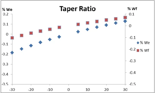
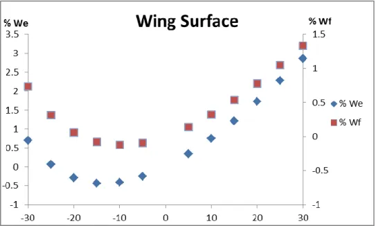
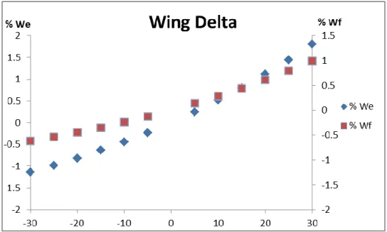
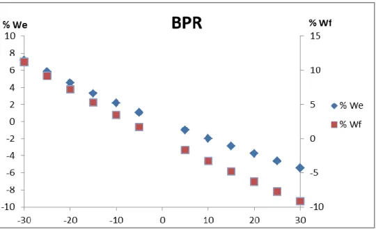
All the graphs can be seen in the annex on the final pages. The first set of figures, with the red markings, refers to the fuel weight variation and the second set, in blue markings, refers to the empty weight variation.

4.2.1 - Mach number

The first variation is the one made to the cruise speed. As said previously, there are five speeds used for this study. The influences are noted, not only on the fuel weight, but also in the empty weight.

We [N] Wf [N] M 0.65 363244 168277 M 0.675 360512 163880 M 0.7 358980 160086 M 0.725 358597 156832 M 0.75 359490 154104

Table 4.1 – Empty and fuel weight for each cruise speed;

As can be seen, the fuel weight has a decrease with cruise speed increase. The same happens with the empty weight, until the last alteration, where a slight increase is noted. In Fig. A.1 is noted that the fuel weight takes its lower value at higher speeds, but the empty weight has its minimum around Mach 0.72.

4.2.2 - Aspect Ratio

Next up is the variation of the aspect ratio. The fuel burned has a decrease with a slight increase in aspect ratio, but only until a certain point. The curve takes a minimum point around 10% to 15% of aspect ratio increase, but returns to 0 from 20% to 30%, setting a superior limit to aspect ratio to the optimized configurations.

As for the empty weight, the effects are similar. The curves minimum is achieved at around 5% to 15% and the weight starts to increase again around 10% to 30%.

The behaviour of both empty and fuel weight with the variation of the aspect ratio along all the cruise speeds can be seen in these contour graphs:

Fig. 4.1 – Contour graph for Wf results through A and Mach number variations;

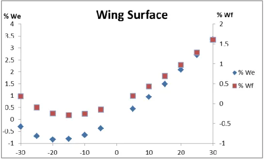
4.2.3 - Wing Surface

The influences of the variations in wing surface area take slightly different shapes as the cruise speed increases. At the lowest and higher speeds, 0.65 and 0.75 respectively, any sort of alteration leads to an increase in fuel burned. On intermediary speeds, a decrease in area leads to a reduced fuel weight. The curves have a minimum around -10% to -20% and the weight starts to increase again around -35% to -20%.

In terms of empty weight, a decrease is experienced at all the cruise speeds. The curves have a minimum around 10% to 20% and the weight starts to increase around -40% to -10%.

The behaviour of both weights can also be visualized through these contour graphs:

Fig. 4.3 - Contour graph for Wf results through Sw and Mach number variations;

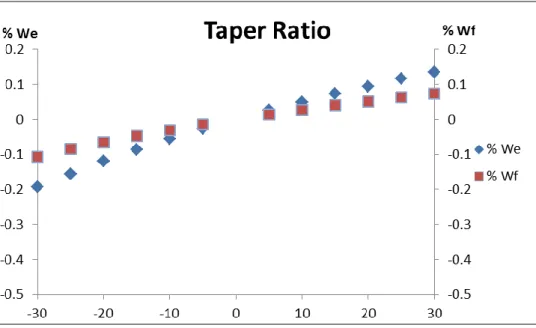
4.2.4 - Wing sweep, taper ratio and bypass ratio

All of these alterations have a very linear behaviour. The lower the wing sweep and taper are set, the lower the fuel and empty weight will be. On the contrary, the more the bypass ratio increases, the lower those two weights are. These results apply both to fuel and empty weight.

4.3 - Optimized versions of the base aircraft

The final step in the study is to find an optimized version for every cruise speed and to analyse the effects of the application of advanced composites on the main structures of the aircraft on both fuel consumption and empty weight.

The purpose of the optimized versions is to understand the effects of the combinations of every kind of variation. As said previously, the limit factors for every version will be the landing and take-off distances and the critical Mach number. Regarding the take-off and landing, the maximum distance has a maximum value of 110% of the distance obtained for the reference aircrafts.

Although there are five different cruise speeds, the results achieved three configurations. The first configuration is the one best suited for the flight at Mach 0.65, 0.675 and 0.7, the second and third are best suited for Mach 0.725 and 0.75, respectively.

AR Sw [m2] _[degrees] Λ λ BPR We Wf M 0.65 10.381 132.927 17.255 0.149 7.8 -6.95% -10.48% M 0.675 10.381 132.927 17.255 0.149 7.8 -6.36% -10.09% M 0.7 10.381 132.927 17.255 0.149 7.8 -5.86% -9.75% M 0.725 10.381 126-281 17.255 0.149 7.8 -6.13% -9.83% M 0.75 10.813 132-927 17.255 0.149 7.8 -4.69% -8.76%

Table 4.2 – Optimized aircraft configurations and performance;

As can be seen above, the wing areas could not assume the optimum value shown in the contour graphs present in figures 4.1 to 4.4. That is due to the fact that the take-off distances would surpass the maximum distances established. Those distance limits are also the reason why the same configuration is optimal for the first three Mach numbers.

As for all the other variables, they all take form or come close to their optimum values. The aspect ratio is a little higher than the recommended by the contour graphs, but the synergy brought by the taper ratio and the wing sweep shift the centre of the graph a bit to the right and increase the value of the optimum aspect ratio.

The visual aspect of each of the three versions and the reference wing can be seen in figure A.32.

4.4 - Advanced composites application

The application of the composites is made to four main components of the aircraft: the wings, fuselage, tails and landing gear. To analyse the effects of each appliance and the several combinations between them, there will be sixteen versions of the optimized aircraft: the one achieved earlier and the fifteen combinations of aircraft with composite components.

Wings Tails Fuselage Landing _gear Version 1

Version 2

Version 3 with composites Version 4 without composites Version 5 Version 6 Version 7 Version 8 Version 9 Version 10 Version 11 Version 12 Version 13 Version 14 Version 15 Version 16

Table 4.3 – Composites application for every version;

All these applications will influence the total weight of the components multiplying their weight by “fudge factor”. Such factors can be found in table 15.4 of reference [9]. Since those multipliers come in a range of values, the select ones were an average of that range. Due to the historical nature of the data [9], some errors of approximation are expected, but it should be good for a rough estimative.

The effects on both the fuel and empty weight can be seen in the graphs from A.27 to A.31. The variations range from the optimized version until the same version with all its main components composed of advanced composites.

We [N] _{We [%]} Wf [N] _{Wf [%]} M 0.65 316787 _-12.789545 145595 -13.4792 M 0.675 316471 _-12.21621 142435 -13.086 M 0.7 316875 _-11.728911 139674 -12.7506 M 0.725 315870 _-11.915038 136771 -12.7913 M 0.75 321281 _-10.628724 135899 -11.8133

Table 4.4 – Fuel and empty weight for every optimized version with full composite application;

As can be seen above, the 0.75 altered version is the worst in terms of both weight reductions compared with the optimized version and in terms of empty weight compared with all the other four versions. But in terms of fuel weight, it is the best version, beating the second best by almost 1000 N, around 110 Kg.

These results are consistent with what has been obtained previously, with the higher cruise speed getting the best results in terms of required fuel weight.

5 – Conclusions

As expected, the BPR variation had the biggest influence on both the empty and fuel weight, as can be seen in the Appendix graphs. The aspect ratio and wing surface variations had some unexpected results, since the increase of the aspect ratio only had the desired results until a certain percentage, after which the empty weight and required fuel would both increase. The same was verified for the surface of the wing, as there was a small interval were the reduction would have a positive impact on the empty and fuel weight, out of which both values would rise. As for the wing sweep and taper ratio, the results came as expected. The increase in velocity led to a decrease in fuel and empty weight. Such results are related to the cruise and divert consumption equation, equation (61), which has the cruise speed on a position where the fuel fraction of those flight phases rises with the cruise speed, granting a lower fuel usage.

All the advanced composites applications have produced the expected results, leading to a reduction in both fuel and empty weight to the optimized version of the aircraft for every cruise speed.

Proposals for future studies

For a future study, it is suggested to create a new calculation tool capable of including types of engine other than the turbo fan used in this study, so its use.is not so limited to only one kind of engine, and that is able to estimate the cost of production and operation. It is also suggested to further study the versions with applied composites in order to optimize those versions.

A major improvement would be to replace the “fudge factors” with some values that do not involve historical data to determine the effects of the application of composites in an aircraft’s components.

References

[1] National Aeronautics and Space Administration; Green Aviation: A Better Way to Treat the Planet;

[2] Xander Olsthoorn; Carbon dioxide emissions from international aviation: 1950-2050; Institute for Environmental Studies (IVM), Vrije Universiteit Amsterdam, De Boelelaan 1115, 1081 HV Amsterdam, Netherlands; Journal of Air Transport Management 7 (2001) 87-93; [3] Wolfgang Lutz, Warren Sanderson and Sergei Scherbov; Doubling of world population unlikely;

[4] R.P. Henderson, J.R.R.A. Martins, R.E. Perez; Aircraft conceptual design for optimal environmental performance; The Aeronautical Journal, January 2012 Vol 116 No 1175;

[5] Nicolas E. Antoine, Ilan M. Kroo; Framework for Aircraft Conceptual Design and Environmental Performance Studies; AIAA JOURNAL, Vol. 43, No. 10, October 2005;

[6] Gaetan K.W Kenway_, Ryan Hendersony, Jason E. Hickenz, Nimeesha B. Kuntawalay, David W. Zingg, Joaquim R. R. A. Martins, Ross G. McKeand; Reducing Aviation's Environmental Impact Through Large Aircraft For Short Ranges, American Institute for Aeronautics and Astronautics;

[7] Bob Saynor, Ausilio Bauen, Matthew Leach; The Potential for Renewable Energy Sources in Aviation; Imperial College Centre for Energy Policy and Technology;

[8] R. H. Liebeck; Design of the Blended Wing Body Subsonic Transport; Journal of Aircraft, vol 41 nº1 January-February 2004;

[9] Daniel P. Raymer; Aircraft Design: A Conceptual Approach; Forth Edition; AIAA Education Series, 01 June 2002;

[10] Denis Howe; Aircraft Conceptual Design Synthesis; Professional Engineering Publishing, 2000;

[11] Anon; Take-off and Landing;www.dept.aoe.vt.edu/~lutze/AOE3104/takeoff&landing.pdf, last checked 29-09-2014;

[12] François de Gernon, Miriam la Vecchia and Alexis Rigaldo; Performance and Design of the Airbus A320 - Analysis of a Subsonic Aircraft; Department of Aerospace and Vehicle Engineering, Royal Institute of Technology - SE 114 15 Stockholm, Sweden;

Appendix

Fig. A.1 – Fuel and empty weight variation in Newton through the tested cruise speeds;

Fig. A.2 – Fuel and empty weight variation due to Aspect Ratio at M 0.65;

Wf /Wf_ref = (A/A_ref)^4 * 8*10^-7 - (A/A_ref)^3 * 4*10^-5 + (A/A_ref)^2 * 0.0053 - (A/A_ref)* 0.1411 + 0.0039;

We/We_ref = (A/A_ref)^4 * 8*10^-7 - (A/A_ref)^3 * 5*10^-5 + (A/A_ref)^2 * 0.0032 - (A/A_ref) * 0.0831 + 0.0049;

Fig. A.3 - Fuel and empty weight variation due to Wing Surface at M 0.65;

Wf /Wf_ref = (Sw/Sw_ref)^4 * 3*10^-7 - (Sw/Sw_ref)^3 * 2*10^-5 + (Sw/Sw_ref)^2 * 0.0011 - (Sw/Sw_ref) * 0.0102 + 0.0014;

We/We_ref = (Sw/Sw_ref)^4 * 5*10^-7 - (Sw/Sw_ref)^3 * 3*10^-5 + (Sw/Sw_ref)^2 * 0.0019 - (Sw/Sw_ref) * 0.0359 + 0.0025;

Fig. A.4 - Fuel and empty weight variation due to Wing sweep at M 0.65;

Wf/Wf_ref = (Δ/Δ_ref)^2 * 0.0002 + (Δ/Δ_ref) * 0.0288 – 0.0005;

Fig. A.5 - Fuel and empty weight variation due to Taper Ratio at M 0.65;

Wf/Wf_ref = -(λ/ λ_ref)^2* 2*10^-5 + (λ/ λ_ref) * 0.0028 + 0.0001;

We/We_ref = -(λ/ λ_ref)^2 * 3*10^-5 + (λ/ λ_ref) * 0.0052 + 0.0002;

Fig. A.6 - Fuel and empty weight variation due to Bypass Ratio at M 0.65;

Wf/Wf_ref = (BPR/BPR_ref)^2 * 0.0013 - (BPR/BPR_ref) * 0.3498 – 0.0027;