Vol. 34, No. 03, pp. 873 – 883, July – September, 2017 dx.doi.org/10.1590/0104-6632.20170343s20150663
* To whom correspondence should be addressed
EFFICIENT NUMERICAL METHOD FOR
SOLUTION OF BOUNDARY VALUE PROBLEMS
WITH ADDITIONAL CONDITIONS
Mirosław K. Szukiewicz¹
¹Rzeszów University of Technology, Department of Chemical and Process Engineering, al. Powstańców Warszawy 6, 35-959 Rzeszów, Poland
E-mail: [email protected]
(Submitted: October 20, 2015; Revised: February 2, 2016; Accepted: March 12, 2016)
Abstract – An efficient numerical method for solution of boundary value problems with additional condition is presented. The approach is based on the shooting method but the procedure of seeking “the proper shot” allows one to satisfy “additional” boundary conditions. General considerations are illustrated by a real example. The computational example concerns the “dead zone” regime for the non-linear diffusion-reaction equation in heterogeneous catalysis. Accuracy and efficiency of the presented method confirm results obtained for a wide range of changes of process parameters, including the vicinity of a critical point. Calculations were performed with the use of the Maple® program.
Keywords: numerical algorithm, BVP with additional conditions, dead zone, CAS-type programs.
INTRODUCTION
Shooting methods, finite difference methods, volume
methods and orthogonal collocation methods are
numerical approaches usually employed for solution of chemical engineering boundary-value problems. The methods are rather well-known and their descriptions
and applicability in chemical engineering are widely
reported in research articles and books, e.g., Davis (1984). However, there are cases in which applicability of the mentioned methods is limited and/or inconvenient. To my mind, the most recognizable problem of this type in chemical engineering is the Stefan problem in which a phase boundary can move with time. The Stefan problem is an example of a free boundary problem. One can find it in fluid mechanics, combustion, filtration and other fields of chemical engineering. It is worth noting that the
most popular mathematical programs such as Matlab,
Maple, Mathematica currently do not support this type of calculations. Nevertheless, these programs are very useful
– many authors implement their own algorithms (e.g. recently published Matlab procedures given by Campo and Lacoa, 2014 or Johansson et al., 2014). Another problem
demanding an additional condition is presented here,
the problem of an ordinary differential equation with an unknown domain. A task is mathematically related to a nonlinear Stefan problem - it can be treated as its stationary version. A dead zone problem in heterogeneous catalysis is a practical application example. The dead zone regime in
catalyst pellets will be presented in the next point.
The algorithm presented here is based on the shooting
method. The shooting method converts the boundary value problem (BVP) into an initial value problem (IVP) with all the conditions specified at the initial point. The
missing initial condition was assumed, and the resulting
IVP is solved for numerous initial conditions (trial and error). The BVP problem can be reduced to work out an efficient method of finding the proper value of the missing
initial condition. The procedure proposed here can be
divided on two steps. First, one should find the range in
of Chemical
Engineering
ISSN 0104-6632
Printed in Brazil
which the solution lies. Next, the size of the range found is gradually reduced to obtain satisfactory accuracy. Solving the IVP problem and inspection of results are necessary in each step. Any numerical method of IVP integration and any method of size reduction of the interval in which the
initial condition must lie can be used. Calculations were
performed with the use of the Maple® program. Author’s preferences will be presented.
FOUNDATIONS OF THE DEAD ZONE PROBLEM
The term “dead zone” was introduced by Temkin (1975), to describe the part of a pellet where the reaction does not occur. One of the reasons for the dead zone formation is lack of reagents in a porous catalyst center.
The problem was mentioned and presented also by Aris
(1975), and it has been recently discussed by York et al. (2011) and Andreev (2013). York has examined the case of a dead zone formation for catalyst pellets of different geometries in which a simple irreversible reaction A→R takes place while the kinetic equation is of a power-law type. He showed that the dead zone appears if -1<n<1 and a Thiele modulus value is sufficiently large, i.e., for Φ>Φc, where Φc is the critical value of the Thiele modulus.
For Φ<Φc the reactant concentration in the center of the pellet is positive and a dead zone is absent; for Φ=Φc
concentration in the pellet center drops to zero value and a dead zone is also absent. These two cases are outside of our interest. ForΦ>Φc, the reactant concentration is equal
to 0 within the range (0, x0); this range is the “dead zone”
which appears in the pellet. x0 is an unknown coordinate of
the end of the dead zone.
The conditions for the formation of dead zones require detailed consideration. The first of the conditions, namely -1<n<1 is the necessary condition for a power-law kinetic equation. It must be satisfied, otherwise the concentration inside a catalyst pellet will always be greater than zero and the dead zone will not appear. But this condition does not guarantee dead zone formation. It is insufficient. Only simultaneous fulfilling of the second condition (Φ>Φc) guarantees that a dead zone will appear. The large
set of common types of kinetic equations and necessary conditions is presented by Andreev (2013). Unfortunately, there is not enough available information on sufficient conditions. They have been published only for power-law type kinetics by York (2011) and much earlier by Garcia-Ochoa and Romero (1988) for the simplest reaction (A→R), and for more complex cases (e.g., consecutive parallel reaction) by Andreev (2013). One can conclude that, in many practical cases, sufficient conditions for dead zone formation are unavailable. It is an uncomfortable situation for investigators, it is not known in advance
which model should be put in practice: whether the regular
model (simple for solution, with two boundary conditions)
or the dead zone model (free boundary problem, quite-hard for solution) especially as improper use can lead to serious errors. For this reason it is particularly important to have an opportunity to determine the critical value of the module Φc.
A mass-balance of steady-state diffusion with an irreversible isothermal chemical reaction A→R is described by (in dimensionless terms):
0
2 2 2
f
c
dx
dc
x
a
dx
c
d
where a=0 for slab, a=1 for cylindrical and a=2 for spherical geometry of the pellet.
When a dead zone appears in the pellet, the boundary
conditions are described by:
0
0
x
x
dx
dc
( )
1
=
1
c
Coordinate x0 is determined by an additional condition, namely:
( )
x
0=
0
c
To my best knowledge there is no general analytical solution known for the problem of a dead zone. Numerical solution of that problem is quite difficult because there is not known a point in the middle of a pellet, when a dead zone begins.
Equations (5) – (7) present the analytical solution for boundary value problem (1)-(4) for typical geometries (a = 0, 1, 2) and a power-law kinetic function (York et al., 2011 and Andreev, 2013).
( )
c
c
nf
=
+
−
+
−
=
Φ
a
n
n
n
c1
1
1
2
(
)
nx
c
The solution presented will be helpful in further parts of the paper.
ALGORITHMS
A simple inspection of the “dead zone” problem (eqs. (1) – (4)) shows that the equations (1), (2) and (4) describe
a typical IVP and the solution can be obtained by choice
of the value of x0 (e.g., using a trial and error method). Unfortunately, if x0 is chosen as a starting point of integration, one can obtain only a trivial solution (c(x)=0).
For this reason it is necessary to use more sophisticated
procedure. It is purposeful to defi ne a new independent variable:
x
z
=
1
−
Consequently, it rearranges eqs. (1)-(4) into:
Let α denotes a value of the derivative of concentration with respect to z evaluated at the point z=0 (missing initial condition) and let the unknown α0 be the value for which the conditions (10) and (12) are satisfi ed. Then:
0 zdz
dc
It is easy to show that it corresponds to the original problem:
Thus, eq. (9) with initial conditions (11) and (13) and an assumed α-value is an IVP-problem to solve. Parameter α should be changed until the conditions (10) and (12) will be satisfi ed simultaneously (in contrast to the “normal”
shooting method, where only one boundary condition must
be satisfi ed). A simple inspection of eq. (6) shows that the value of α should be negative, that is α0-values are included
in the interval (-∞,0).
Main procedure of α0-value seeking (algorithm A)
Let us assume that a dead zone in the pellet exists and the problem has a single solution (the usual case). This condition is satisfi ed inter alia by the following data:
( )
c
=
c
1/2;
a
=
0
;
Φ
=
4
f
According to (5)-(7), for this data one can obtain:
3
3
8
;
2
3
1
;
1
3
3
2
1
;
3
2
1
0
4
x
dx
dc
x
x
c
c
2
3
;
1
2
3
3
1
;
1
2
3
;
8
3
3
1
0
4
x
dx
dc
x
x
c
c
3
3
8
;
2
3
1
;
1
3
3
2
1
;
3
2
1
0
4
x
dx
dc
x
x
c
c
Taking into account the above solution, the proper guess for the eq. (9) is:
0
0
3
3
8
z
dz
dc
The IVP should be integrated from point z=0 until the concentration or its derivative achieves zero; further integration has no sense - conditions (10) and (12) cannot be satisfi ed simultaneously. It results from the accepted assumption that a dead zone in the pellet exists; if concentration or its derivative do not achieve zero within
the tested range, it can be concluded with high probability
that a dead zone does not appear for the tested data (e.g., the Thiele modulus value is too small).
As can be seen in the results, the concentration decreases
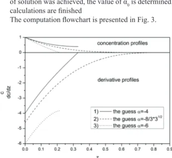
monotonically from unity, while the derivative increases monotonically from the initial value. As it was mentioned the α0-value seeking procedure is based on the inspection of results of integration of the IVP: eq.(9), with conditions eq.(11) and (13). First, three types of the IVP solutions depending on the α-value will be presented (see Fig. 1):
● if the concentration derivative achieves zero while the concentration is still positive, too high a value of the guess has been assumed - see solid lines in Fig. 1; this type of solution will be called further T1
● if the concentration and its derivative achieve zero for the same z-value, the proper value of the guess was assumed - see dashed lines in Fig. 1; this type of solution will be called further T2
● if the concentration achieves zero while the derivative is still negative, too small a value of the guess was assumed - see dotted lines in Fig. 1; this type of solution will be called further T3.
To achieve satisfactory accuracy, the proposed method of determining the type of solution should be sensitive with respect to changes of the α-values. The lines presented in Fig. 2 confirm this fact: the profiles for two very close values of α: α=-4.6188 and α=-4.6189 (-4.6188>α0>-4.6189) are significantly differ. It
shows that the considered method allows one to obtain the
missing initial condition value with a high precision. The algorithm of seeking the proper value of the initial guess is presented as follows:
1. The initial value of α can be arbitrarily chosen. Equation
(9) should be integrated and the obtained solution should be qualified as T1 or T3. It determines the upper (αH) or the lower limit (αL) of the interval in which α0 must lie, respectively.
2. The next step
a) If the αH-value has been determined, the T3 type of solution can be obtained by decreasing α and integration of eq. (9). This determines the lower limit (αL) of the interval in which α0 must lie.
b) If the αL-value has been determined, the T1 type
of solution can be obtained by increasing α and integration of eq. (9). This determines the upper limit (αH) of the interval in which α0 must lie.
3. The next guess should satisfy condition αL<α<αH.
Integration of eq. (9) allows one to determine the type of solution for the current value of α.
a) if the current value of αgives a solution of the T1 type, we have found another new value of αH
b) if the current value of α gives a solution of the T3 type, we have found another new value of αL.
As a result the size of the interval (αL; αH) is reduced. This
procedure should be repeated until the difference αH-αL
becomes satisfactorily small; it determines the value of α0within the required tolerance.
4. If, sporadically, in any of the above points the T2 type
of solution was achieved, the value of α0 is determined; calculations are finished
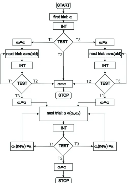
The computation flowchart is presented in Fig. 3.
Multiple steady states (algorithm B)
If multiple steady states exist, more than one value of α0 can be found in the interval (-∞,0). Using different trials Figure 2. Concentration and its derivative vs. distance inside the
pellet; sensitivity of the algorithm.
Figure 3. Computation flowchart; INT=integration of IVP, TEST=examination of the solution type.
of initial values of α one can find all possible solutions. Remark: for a stable solution the proposed algorithm does not change, while for an unstable solution, the types T1 and T3 have the reversed meaning.
A dead zone does not exist (algorithm C)
The algorithm presented in the previous points, after minor modifications, allows one to find a solution also in this case. The algorithm scheme (Fig. 3) remains unchanged, integration limits and the description of the types of solutions should be slightly modified:
● the IVP should be integrated from z=0 until z=1; values of the concentration and its derivative for z=1 should be tested
● if the derivative is positive (at z=1), too high a value of the guess has been assumed (it corresponds to T1)
● if the concentration is positive or equal to zero and its derivative is zero for z=1, the proper value of the guess has been assumed (it corresponds to T2) ● if the concentration is positive while the derivative
It was pointed out that the case without the dead zone in the pellet is out of our interest: x0=0 and then the problem
reduces to a typical two-point boundary value problem. However, there is an important reason to present a suitable procedure here. It was mentioned that a dead zone can be formed only for particular types of kinetic equations, but the set of sufficient conditions for dead-zone formation has not been developed (with exceptions presented in point 2). For this reason it is difficult to predict whether to use a model with a dead zone or not,while improper use can lead to serious errors. Thus, if the sufficient conditions are not available, I recommend to use a combination of the algorithms A and C to determine a regime of catalyst pellet work (dead zone exists or not). In other words, it is possible to determine the missing sufficient condition for dead zone existence, that is to calculate Φc. This is a rather
simple task, due to the similarity of algorithms.
RESULTS AND DISCUSSION
The calculation procedure was implemented by the
author in Maple®, using a stiff version of the Rosenbrock algorithm for IVP solution (internal procedure of Maple®) and the bisection method as a method of reduction of the size of interval (αL, αH). The final value of the difference
(αH-αL) was not larger than 10 -18.
The effectiveness factor was calculated as follows
1
2
1
xdx
dc
a
First, the accuracy of the method was verified by
comparing:
● the values of the effectiveness factor; ηnum calculated
numerically and ηan calculated analytically using eq. (5)-(7) and (18)
● the values of the dead zone-end; x0,num calculated
numerically and x0,an calculated analytically using eq.
(5)-(7) and (18)
for a=0 and different values of parameters Φ and n. Coefficients were calculated up to 5 decimal places.
Results are presented in Table 1. The precision of the calculations is very high. The results agree up to the fifth decimal place, with the only exception for n=-1/2 and Φ=0.66667. The relative error is equal to 0.002 (0.2%). Explanation of this exception requires analysis of the equation considered. Thus, if n is negative then the point at Φ=Φc is singular and accuracy of numerical procedures in the vicinity of critical point decreases.
The results show that the accuracy of the method considered is very high, and, most likely, only in the vicinity of critical points does the accuracy drop down. To confirm this observation, the next test was made, the calculation of critical values of the Thiele modulus for different values of the parameter n. For elementary pellet geometries (a=0, 1, 2),
we compared:
● the critical values of the Thiele modulus Φc,num calculated numerically and Φc,an calculated analytically
using eq. (5)-(7) and (18)
● the values of the effectiveness factor for the critical value of the Thiele modulus ηc,num calculated numerically and
ηc,an calculated analytically using eq. (5)-(7) and (18)
This test also allows checking the proposed algorithm as an effective tool to calculate the critical Thiele modulus. Coefficients were calculated up to 5 decimal places.
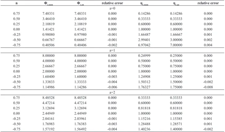
Results are presented in Table 2. For n≥0 calculations are errorless, while for n<0 the computed values of Φc and ηc are not as accurate. This observation confirms the hypothesis presented above that the algorithm accuracy drops down only in the vicinity of critical points. The errors are not large for the specified tolerance– they are less than 1%. Errors grow as n decreases. The results show that the algorithm presented allows one to determine the sufficient condition of dead zone existence with satisfactory accuracy.
Rather unexpectedly, the dead zone can appear in real processes relatively often. Methanol steam reforming over
a commercial Cu/ZnO/Al2O3 catalyst will be considered
as a practical example for application of the method proposed here. Hydrogen production from hydrocarbon steam reforming is a cost-effective method for providing hydrogen; methanol steam reforming is a simple and efficient way of producing hydrogen on a small scale:
kJ
H
H
CO
O
H
OH
CH
3
2
2
3
2;
473K
57
The kinetic equation, catalyst data and process data
were reported by Lee et al. (2004). They proposed the following kinetic equation at atmospheric pressure and in a temperature range between 433 and 533K:
s
kg
mol
p
kPa
p
RT
mol
kJ
r
M2
.
19
10
9exp
103
/
M0.56411
.
6
H 0.647;
(18)
Table 1. Comparison of results obtained numerically with the exact solution - effectiveness factor and dead zone-end.
Φ ηnum ηan x0,num x0,an
n=0.5, Φc=
3.46411 0.33333 0.33333 0.00000 0.00000
4.0 0.28868 0.28868 0.13397 0.13397
5.0 0.23094 0.23094 0.30718 0.30718
6.0 0.19245 0.19245 0.42252 0.42265
8.0 0.14434 0.14434 0.56699 0.56699
10.0 0.11547 0.11547 0.65359 0.65359
15.0 0.07698 0.07698 0.76906 0.76906
n=0.25, Φc=
2.10819 0.60000 0.60000 0.00000 0.00000
2.5 0.50596 0.50596 0.15673 0.15673
4.0 0.31623 0.31623 0.47295 0.47295
6.0 0.21082 0.21082 0.64864 0.64864
8.0 0.15811 0.15811 0.73648 0.73648
10.0 0.12649 0.12649 0.78918 0.78918
15.0 0.08433 0.08433 0.85945 0.85945
n=-0.5, Φc=
0.66667 2.99401 3.00000 0.00000 0.00000
0.7320 2.73224 2.73224 0.08925 0.08925
0.7870 2.54130 2.54130 0.15290 0.15290
0.8320 2.40385 2.40385 0.19872 0.19872
0.8870 2.25479 2.25479 0.24840 0.24840
0.9400 2.12766 2.12766 0.29078 0.29078
1.0 2.00000 2.00000 0.33333 0.33333
2.0 1.00000 1.00000 0.66667 0.66667
5.0 0.40000 0.40000 0.86667 0.86667
Table 2. Comparison of a critical value of the Thiele modulus and effectiveness factor obtained numerically with the exact solution. n Φc,num Φc,an relative error ηc,num ηc,an relative error
a=0
0.75 7.48331 7.48331 0.000 0.14286 0.14286 0.000
0.50 3.46410 3.46410 0.000 0.33333 0.33333 0.000
0.25 2.10819 2.10819 0.000 0.60000 0.60000 0.000
0.00 1.41421 1.41421 0.000 1.00000 1.00000 0.000
-0.25 0.98080 0.97980 -0.001 1.66487 1.66667 0.001
-0.50 0.66767 0.66667 -0.001 2.99401 3.00000 0.002
-0.75 0.40506 0.40406 -0.002 6.97042 7.00000 0.004
a=1
0.75 8.00000 8.00000 0.000 0.24999 0.25000 0.000
0.50 4.00000 4.00000 0.000 0.50000 0.50000 0.000
0.25 2.66667 2.66667 0.000 0.75000 0.75000 0.000
0.00 2.00000 2.00000 0.000 1.00000 1.00000 0.000
-0.25 1.60400 1.60000 -0.003 1.24908 1.25000 0.001
-0.50 1.33833 1.33333 -0.004 1.50312 1.50000 -0.002
-0.75 1.14986 1.14286 -0.006 1.76327 1.75000 -0.008
a=2
0.75 8.48528 8.48528 0.000 0.33333 0.33333 0.000
0.50 4.47214 4.47214 0.000 0.60000 0.60000 0.000
0.25 3.12694 3.12694 0.000 0.81818 0.81818 0.000
0.00 2.44949 2.44949 0.000 1.00000 1.00000 0.000
-0.25 2.04161 2.03961 -0.001 1.15216 1.15385 0.001
-0.50 1.76983 1.76383 -0.003 1.28488 1.28571 0.001
-0.75 1.57192 1.56492 -0.004 1.40236 1.40000 -0.002
3.46411 3
2 ≈
2.10819 3
/ 10
2 ≈
0.66667
3
/
2
≈
The concentration profile of methanol and the hydrogen
inside a catalyst particle depend upon each other by the
following mutual relation:
Ms M
H e
M e Hs
H
y
D
D
y
y
y
, ,
3
so that pH can be removed from eq. (20). As a result, the
methanol concentration profile and effectiveness factor can be determined from a single mass balance equation (1) with appropriate boundary conditions (either (2)-(4), if a dead zone exists, or (2)-(3) and x0=0, if a dead zone does not exist). Catalyst properties, gas compositions and effective diffusivity of methanol and hydrogen are taken from the article mentioned.
The Thiele modulus Φ is defined by:
M e Ms
M
D
c
r
, 2
Let us consider the following case. Andreev (2013) showed that, for a power-law kinetic equation, a dead zone can exist in a catalyst pellet. A necessary but insufficient condition is 1<n<1, where n is an exponent in the kinetic equation. A sufficient condition for eq. (20) is unavailable, additionally due to the atypical form of the equation (the hydrogen partial pressure term in the
power-law expression is corrected by a constant); it cannot be determined whether the necessary condition is satisfied or not. However a presumption that a dead zone appears in the catalyst pellet is very likely – absolute values of the exponents in eq. (20) are less than 1. The presumption will be confirmed computationally. The algorithm described will be very useful – one can examine the validity of boundary conditions and next calculate the critical value of
the Thiele modulus without a trial and error method.
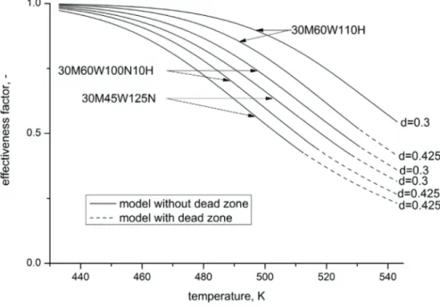
Calculations were performed for catalyst diameters of 0.3mm and 0.425mm (extreme diameters of commercial catalysts reported by the manufacturer), average values of effective diffusivities and three feed compositions 30M45W125N (yMs=15 mol%, yHs=0), 30M60W100N10H (yMs=15 mol%, yHs=5 mol%) and 30M60W110H (yMs=15 mol%, yHs=55 mol%). Results
are presented in Fig. 4 and Fig.5. In Fig. 4 are presented
the effectiveness factors vs. temperature for different gas
compositions and catalyst diameters. In Fig.5 the same
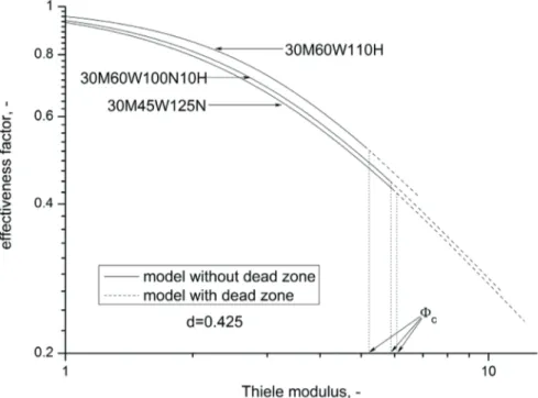
results (only for d=0.425mm) are presented in a more convenient form, i.e., effectiveness factor vs. Thiele modulus. Regardless of gas composition the curves are
similar. The methanol concentration decreases towards the
center of the pellet more rapidly the faster the reaction runs, i.e., for higher temperature. For a certain temperature, the methanol concentration in the center drops to zero and for higher temperatures a dead zone is formedin the pellet center. This fact is illustrated in Figures 4 and 5: solid lines for a regular solution change into dash lines for a dead zone solution. For this region the free boundary problem (equations (1)-(4)) has to be used.
Figure 4. Effectiveness factor vs. temperature for various feed compositions and catalyst diameters.
(21)
Figure 5. Effectiveness factor vs. Thiele modulus for various feed compositions
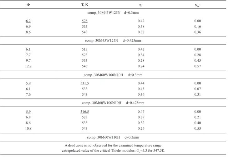
It is clear that, for the considered process, a dead zone appears in each case. A dead zone is observed for temperatures higher than 513K. This temperature range corresponds to high methanol conversion and, for this reason, to improve productivity of the process, the possibility of formation of a dead zone should be taken into account. For further analysis more detailed results are presented in Table 3. The Thiele modulus values and the corresponding temperatures, effectiveness factors and coordinate of the zone-end (the greater the value of coordinate the larger the dead zone) are presented there. Critical values of the Thiele modulus are underlined. The
presented results show that a higher temperature and larger
catalyst pellets are conducive to the appearance of a dead zone. This is understandable because diffusion resistance grows in the catalyst. From a practical point of view, the following observations are:
● the estimated critical values of the Thiele modulus on the basis of experimental results are practically the same for the same gas compositions; it means that the Φc-value is characteristic for the kinetic equation,
because for different catalyst diameters the critical value of the Thiele modulus is approximately constant; this fact confirms the hypothesis previously presented by Temkin (1975) and Aris (1975).
● The dependence of the critical modulus on the composition of the mixture is significant
● it may be observed that some pellets in the catalyst bed can work in the normal regime (diffusional), while a dead zone appears in others, e.g., if T≈530K, the catalyst works normally at a high content of hydrogen (it corresponds to the reactor outlet conditions), while a dead zone fills 10-40% of the catalyst pellets at low content of hydrogen (it corresponds to the reactor inlet conditions);
Detailed analysis could help to improve productivity of the process, but it is not the aim of the present study.
The discussed case of methanol steam reforming shows that the method presented is useful and effective for analysis of a real, complex process. It helps to improve understanding of the process and to adjust process conclusions to common knowledge.
The tests made show that the algorithm proposed here
is simple and precise both for theoretical considerations and practical purposes. High efficiency and high accuracy of the calculations is ensured by correct selection of the
numerical method, while the ability to use any methods
makes the algorithm “flexible” and it can be easily
Table 3. Dead zone formation in the catalyst pellets for methanol steam reforming.
Φ T, K η- xdz
-comp. 30M45W125N d=0.3mm
6.2 6.9 8.6
528 533 543
0.42 0.38 0.32
0.00 0.16 0.36
comp. 30M45W125N d=0.425mm
6.1 7.7 9.7 12.2
513 523 533 543
0.42 0.34 0.28 0.24
0.00 0.28 0.45 0.57
comp. 30M60W100N10H d=0.3mm
5.9 6.1 7.6
531.5 533 543
0.44 0.43 0.36
0.00 0.07 0.31
comp. 30M60W100N10H d=0.425mm
5.9 6.8 8.6 10.8
516.5 523 533 543
0.44 0.39 0.32 0.26
0.00 0.21 0.40 0.53
comp. 30M60W110H d=0.3mm
A dead zone is not observed for the examined temperature range extrapolated value of the critical Thiele modulus: Φc=5.3 for 547.5K
comp. 30M60W110H d=0.425mm
5.2 5.5 6.8
531 533 543
0.51 0.50 0.41
0.00 0.06 0.30
CONCLUSIONS
On the basis of the results presented the following
conclusions can be drawn:
the algorithm is simple – it relies on a shooting
method; an iterative approach to finding the missing initial condition was presented;
the algorithm is “flexible” and effective - it enables one to take advantages of numerous numerical methods; for this reason, it makes it possible to obtain results of high precision in a wide range of model parameter values, also in the vicinity of critical points;
the algorithm is also useful in the multiplicity region for computation of both stable and unstable solutions
the algorithm can be easily implemented for real tasks with an “additional boundary condition”; e.g. the presented dead zone problem in heterogeneous catalysis, but also for
other problems inter alia grain hydration or a characteristic
task in mechanics: the normal reaction in the plane of the curve for particle motion
ACKNOWLEDGMENTS
The financial support of the National Science Centre, Poland (Project 2015/17/B/ST8/03369) is gratefully acknowledged.
NOMENCLATURE
C [-] –concentration
cM [mol/m3] –methanol concentration on the surface
De [m2/s] –effective diffusivity
n [-] –exponent
p [kPa] –partial pressure R [J/(mol K)] –gas constant
T [K] – temperature
x [-] – spatial coordinate x0 [-] – dead zone-end coordinate
y [-] – mole fraction z [-] – spatial coordinate Greek
Φ [-] – Thiele modulus η [-] – effectiveness factor ε [-] – void fraction
α [-] – value of derivative of concentration with respect to z evaluated
at the point z=0 ρ [kg/m3] – catalyst density
α0 [-] – proper value of the missing
initial condition
Φc [-] – critical Thiele modulus αH [-] – upper limit of α0
αL [-] – lower limit of α0
Superscripts
an – analytical solution
H – hydrogen
M – methanol
num – numerical solution
s – pellet surface
REFERENCES
Andreev V.V., Formation of a “Dead Zone” in Porous Structures During Processes That Proceeding under Steady State and
Unsteady State Conditions, Review Journal of Chemistry, 3, No. 3, 239 (2013).
Aris. R., The Mathematical Theory of Diffusion and Reaction in Permeable Catalysts. Vol I. The Theory of the Steady State. Clarendon Press, Oxford (1975).
Campo A. and Lacoa U., Adaptation of the Method Of Lines (MOL) to the MATLAB Code for the Analysis of the Stefan Problem, WSEAS transactions on heat and mass transfer, 9, 19, (2014).
Davis M. E., Numerical Methods and Modeling for Chemical Engineers. Wiley, New York (1984).
Garcia-Ochoa F., Romero A., The Dead Zone in a Catalyst Particle for Fractional-Order Reactions, AIChE J., 34, 1916-1918, 1988
Johansson B.T., Lesnic D. and Reeve T., A meshless method for an inverse two-phase one-dimensional nonlinear Stefan problem, Mathematics and Computers in Simulation, 101, 61, (2014).
Lee J. K, Ko J.B., Kim D.H., Methanol steam reforming over Cu/ZnO/Al2O3 catalyst: kinetics and effectiveness factor, Applied Catalysis A: General 278 (2004) 25–35.
Magyari E., Exact analytical solution of a nonlinear reaction-diffusion model in porous catalysts, Chem. Eng. Journ., 143, 167 (2008).
Temkin M.I., Diffusion Effects During the Reaction on the Surface Pores of a Spherical Catalyst Particle, Kinet. Cat., 16, 104 (1975).