Educação
*e-mail: [email protected]; [email protected]
REVISITING IDEAL GASES AND PROPOSAL OF A SIMPLE EXPERIMENT FOR DETERMINING ATMOSPHERIC PRESSURE IN THE LABORATORY
Leonardo M. Da Silva* and Arthur H. de Castro
Departamento de Química, Universidade Federal dos Vales do Jequitinhonha e Mucuri, Rodovia MGT 367, km 583, 5000, Alto da Jacuba, 39.100-000 Diamantina – MG, Brasil
Recebido em 15/12/2017; aceito em 08/03/2018; publicado na web em 29/03/2018
Relevant historical aspects concerning ideal gases were briefly reviewed to provide a condensed resource for the undergraduate student of chemistry. The importance of the barometer and the concept of atmospheric pressure were reviewed and discussed. A combination of Boyle’s law with the well-known equation for determining the pressure produced by a column of stationary fluid was used to obtain a graphical method for determining atmospheric pressure under isothermal conditions in the laboratory. Important aspects related to the study of ideal gases were reviewed in light of the pressure-volume data that can be obtained by physical chemistry students using a simple apparatus composed of a commercial hypodermic syringe connected to a mercury manometer. Relevant concepts associated with the measurement of a physical quantity, the importance of linear regression, as well as the use of a graphical method to test the validity of a theory were reviewed from a pedagogical perspective through the experimental study of Boyle’s law during regular experimental physical chemistry classes.
Keywords: ideal gases; Boyle’s law; atmospheric pressure; hypodermic syringe; experiments in physical chemistry.
INTRODUCTION
Matter can be roughly divided into three main categories, namely gases, liquids, and solids. In this classification scheme, the ‘rarefied gases’ are a simplified gas state, commonly known as ‘perfect’ or ‘ideal’ gases, which obey some basic limiting laws.1-12 In the modern picture of the gaseous state, a gas confined at low pressures has molecules that are so far apart that they exhibit only slight attraction to each other, permitting the gas to expand and completely fill a vessel of any size or shape.4 In addition, the physical behavior of a gas confined at low pressures (p < 1−2 atm) and ordinary temperatures (far from the condensation point) is not affected by the chemical nature of the molecules. Thus, all gases respond in nearly the same way to the state variables (pressure, volume, and temperature). Strictly speaking, in the model of an ‘ideal gas’ there is no interaction between molecules, and the internal energy of the gaseous material remains unchanged if the gas is expanded into a larger volume under isothermal conditions.1-12 In this sense, a ‘gas law’ is a mathematical formula which expresses the relationships between pressure, volume, and temperature, which have been found experimentally.1-12
Significant advances in the study of the rarefied gases were first obtained in the 17th century from 1643−1662.1,13-15 In this sense, Galileo’s pupil in Florence, the mathematician Evangelista Torricelli (1608−1647), showed in 1643 that mercury in a vertical tube sealed at one end sank to a height of 30 inches, leaving a vacuous space above which was called a “Torricellian vacuum”.1,14,15 Torricelli suggested that the mercury column in this apparatus, which Robert Boyle (1627–1691) named a ‘barometer’, is sustained by the pressure of the atmosphere on the surface of the mercury in the open dish in which the tube stands.1,14,15 The important studies comprising the pressure-volume behavior of rarefied gases are due to Boyle, 1,13-15 as will be extensively discussed in this article. Additional important advances in the study of the rarefied gases considering the influence of temperature were not obtained until the 18th century (c.a. 1787−1802).1,14,15
Revisiting Boyle’s law: some important peculiarities
The invention of the ‘air pump’ by Otto von Guericke (1602– 1686) in 1650 and his many experiments created an impetus for researchers to study the “vacuum” (actually, a gas confined at a pressure lower than atmospheric pressure).1,14,15 Most noteworthy is Robert Boyle’s work using air as the gaseous substance.1,15 With his mechanically-minded assistant Robert Hooke (1635−1703), Boyle designed and constructed an air pump called a “pneumatical engine”, which was superior to that used by von Guericke.1,14,15 During the period of ca. 1655−1660, Boyle first proved that air had weight and that the height of the mercury column in a barometer varies slightly from day to day. Therefore, atmospheric pressure is not constant at a given location.1,2
The first experiments leading to a ‘gas law’ were performed by Boyle during 1660−1662 using a large J-tube made of glass and partially filled with mercury. Boyle reported in 1662 that the volume (V) of air decreases when pressure (p) is applied, and that the volume is inversely proportional to the applied pressure. This experimental result can be expressed mathematically using the following equation (Boyle’s law):1-15
pV = k, (1)
where k (in units of pressure × volume) is a constant for a fixed mass of air (e.g., number of moles (n), in the modern view). It is worth mentioning in Boyle’s time, the concept of ‘temperature’ was not well developed and, therefore, the influence of temperature was not considered in his experiments.1,2 In fact, it was not until about 125 years after Boyle’s experiments that Charles found that the volume of a gas kept at constant pressure is affected by temperature (see further discussion).14,15
pV = k(T,n) (2) Boyle’s law represents one of the first natural laws recognized by scientists.1-4,14,15 However, it is worth noting that Boyle was by no means alone in pondering the gas law described by equation (1). In fact, Boyle himself mentioned that Richard Townely had suggested the theory “that supposes the pressures and expansions to be in reciprocal proportion”.1,14 In addition, there is an apparent controversy in modern literature about the origins of the gas law represented by equation (1). In fact, Boyle’s law is sometimes known as Mariotte’s law in some non-English-speaking countries.1 However, it is worth mentioning that Edme Mariotte (1620–1684) published his work seventeen years after Boyle.1,14,15 Using the same hypothetical description of the behavior of compressed air proposed by Boyle, Mariotte used the explanation of the pressure or “spring” of the air, comparing it with small fleeces of wool of tiny coiled springs.1,14
The law discovered by Boyle, which is strictly valid for rarefied gases, describes a rectangular hyperbola (e.g., a reciprocal curve) in the p vs. V plane. It is difficult, however, to determine whether experimental data accurately fit such a curve, and it is better to express eqs. (1) and (2) as a linear relation. Therefore, the quantitative analysis of the deviations from Boyle’s law must be accomplished using graphical tests (see further discussion).
Revisiting Charles, Gay-Lussac, and Amontons’ laws: the importance of temperature
Important studies after Boyle’s work considered the influence of temperature on gases kept at constant volume or pressure.1,2,14,15 In particular, the studies of Jacques Alexandre César Charles (1746– 1823) in 1787 and Joseph Louis Gay-Lussac (1778–1850) in 1802 led to the formulation of the following empirical law commonly known as Charle’s law or Gay-Lussac’s law:1,14,15
V(t) = V0(1 +αt), (3)
whereα (coefficient of expansion) = 3.66 × 10⁻³ °C−1 and V 0 is the volume of the gas at 0 °C.
Therefore, if equation (3) is valid at all temperatures, the volume at a given temperature in Celsius V(t) should be zero at a temperature t = −1/α = −273 °C. This temperature (‘absolute zero’) is known today7-12 to be −273.15 °C and it plays a central role in thermodynamics.1-12 Although absolute zero has been considered to be only a mathematical phenomenon, thermodynamic studies show that it is a physical reality.1,6-12
From the above considerations, the Charles-Gay-Lussac’s law represented by equation (3) can be rewritten using the ‘absolute (thermodynamic) thermometric scale’ proposed in 1848 by William Thomson (Lord Kelvin) (1824–1907).1,14,15 Use of this absolute scale permits simple conversion of the thermometric temperature measured in Celsius degrees using a ‘gas thermometer’ by the relationship T/K = t/°C + 273.15. Therefore, equation (3) can be rewritten as follows:6-12
V = k(p,n)×T, (4)
where k(p,n) is a constant for a fixed number of moles and at constant pressure.
According to Boyle’s law and Charles-Gay-Lussac’s law, three parameters can be changed for the rarefied (ideal) gases: volume, pressure, and temperature. The preceding laws deal with the relationship between two pairs of variables while the third is held constant. There remains to consider the relationship between the
third pair of variables, pressure and temperature, with volume held constant.3 Evidently, a necessary corollary of the aforementioned laws is that “at constant volume, the pressure of a gas is directly proportional to its absolute temperature”.3 A ‘pressure coefficient’ β was defined based on this:1-3
p(t) = p0(1 + βt), (5)
where β = α from theoretical considerations (see equation 3) and p0 is the pressure of the gas at 0 °C. However, it was verified experimentally1 for air at low pressures that β and α are slightly different (e.g., α−β = 0.05123).
Charles-Gay-Lussac’s law given by equation (5) can alternatively be written as:6-12
p = k(V,n)×T, (6)
where k(V,n) is a constant for a fixed number of moles and at constant volume. Obviously, the validity of eqs. (4) and (6) relies on Boyle’s law being applicable (e.g., low-pressures).
Equation (6) is sometimes known as Amontons’ law.9 In fact, before Charles and Gay-Lussac, Guillaume Amontons (1663–1705) studied in 1702 the pressure of a constant volume of air as a function of temperature. In addition, Amontons developed the first gas thermometer.9 He also estimated that air pressure would approach and then reach zero at −240 °C. Assuming that the ‘absolute pressure’ of a gas cannot be negative, he suggested that this value represents a lower limit of temperature. Unfortunately, the important achievements of Amontons are not included in many standard general chemistry and physical chemistry textbooks.
The correct formulation of the generalized ideal gas law
From the basic laws discussed above a general equation for the rarefied gases that incorporates the three state variables (p, V, and T) can be formulated. Benoît Paul Émile Clapeyron (1799–1864) proposed the ‘generalized ideal gas law’ in 1834, which is sometimes known as Clapeyron’s equation.1,14 The equation is a result of a simple algebraic combination of Boyle’s law, Charles-Gay-Lussac’s law, and the hypothesis of Amedeo Avogadro (1776−1856) proposed in 1811,1,2,15 which states that “equal volumes of gases at the same temperature and pressure contain the same number of molecules regardless of their chemical nature and physical properties”, i.e., V = k(T,p)×n. The generalized ideal gas law can then be written as:1-12
pV = nRT, (7)
where n is the number of moles and R is the ‘general gas constant’ (e.g., R = 8.31447 J K−1 mol−1). Despite the credit given to Clapeyron in several physical chemistry and general chemistry textbooks, according to Partington1 the origins of equation (7) are mainly due to Horstmann.16
That is, while Boyle’s law is valid at constant temperature, the Charles-Gay-Lussac’s law is valid at constant volume. Therefore, a simple algebraic combination does not make physical sense, despite the fact that the final result (equation (7)) is the same in both cases.9,17,18
Boyle’s law and deviations from ideal behavior: real gases
Boyle extensively examined effects on air volume at pressures greater than atmospheric (positive relative pressures) and less than atmospheric (e.g., vacuum – negative relative pressures). In his studies, pressures varied from 3 to 300 cm of Hg.1
For a long time, Boyle’s law was applied only to atmospheric air.1,14,15 Almost one century later other rarefied gases were studied by Joseph Black (1728–1799), Henry Cavendish (1731–1810), and Joseph Priestley (1733–1804).1 In 1799 Martin Van Marum (1750–1837)1,14,15 reported the first decisive deviation from Boyle’s law based on a study of ammonia (NH3(g)) at high pressures. In the case of air, the deviation from Boyle’s law is more difficult to detect since it is only appreciable above 20 atm,1,2 which is why Boyle himself did not perceive any deviation from his law. The degree of deviation from Boyle’s law with the applied pressure is considerably affected by the nature of the gas. However, all gases at sufficiently high pressures shows a deviation from Boyle’s law.1-12
Therefore, it is evident that Boyle’s law is, in fact, a ‘limiting law’, strictly valid only at low pressures.6-12 During the nineteenth century several scientists, particularly Henri Victor Regnault (1810−1878), from 1847-1862, and Émile Hilaire Amagat (1841−1915), from 1880−1893, carefully studied the compressibility of various gases, and it became evident that for ‘real gases’ (e.g., gases at moderate/high pressures) Boyle’s law is only an approximation (i.e., a limiting law).1,2,8
For instance, for a given mass of gas confined under isothermal conditions in a cylinder-piston system connected to a manometer, the degree of deviation from Boyle’s law can be detected by comparing the product of pressure and volume (p × V) expressed as a function of pressure (i.e., a plot of (p × V) vs. p).9 The validity of Boyle’s law is verified in this way by obtaining a constant value of the product p × V = k (see equation 1).
Linearization of equation (2) can also provide a means of identifying deviations from Boyle’s law:19,20
(8) According to equation (8), a p vs. 1/V plot for a gas that obeys Boyle’s law should be a straight line that passes through the origin. Therefore, a curved line or a straight line that does not cross the origin indicates that Boyle’s law is not valid.
Another useful graphical method is based on the linear model given by equation (9):19,20
ln(p) = ln[k(T,n)] – γ×ln(V), (9)
where γ is a dimensionless empirical parameter representing deviations from Boyle’s law. Although this type of analysis is somewhat arbitrary to establish an ‘acceptable’ degree of deviation from Boyle’s law, the use of equation (9) for experimental findings obtained with great precision must yield a straight line with an exponent (γ) very close to one (e.g., γ ≥ 0.995) to support the validity of Boyle’s law.
In typical cases at low pressures (p ≤ 1−2 atm) in ordinary general chemistry and/or physical chemistry laboratories, deviations from ideal behavior can be ignored for practical purposes. In fact, within a pressure range of 1 to 10 atm the deviations from Boyle’s law are less than about 5% for most gases.2 However, for precise experiments conducted by
chemists and chemical engineers deviations from ideal behavior must be identified and quantified to obtain meaningful results.6-11
The study of rarefied gases by undergraduate students and alternative experimental apparatus for verifying the basic laws of ideal gases
Experiments with air or other gases are common in universities for the study of basic gas properties by undergraduate students of chemistry, physics, and engineering. This is evident given the various different experiments involving gases described in laboratory textbooks.20-27
The study of gases is always of interest to teachers who sometimes have ingenious ideas about a new (alternative) configuration for an experimental apparatus. Therefore, in addition to the well-established experiments with gases described in several laboratory textbooks,20-27 additional (alternative) experiments for the study of rarefied gases can be conducted using different experimental approaches. For example, hypodermic syringes have been used for exploring the physicochemical properties of gases at low pressures.28-35 Davenport28 reported some studies using a 30-mL syringe over a pressure range of about 0.25 to 3 atm. Surprisingly, without a conventional U-tube manometer partially filled with mercury, this author used ‘identical textbooks’ (m = 904 g) that were either piled on or suspended from a syringe plunger to change the pressure of a confined gas. For different gases a plot of p vs. the ‘number of books’ was verified to be linear, confirming p × V = k as proposed by Boyle.
Blanco and Romero35 reported an experimental set up for the systematic study of the physicochemical properties of the ideal gases. However, for verifying Boyle’s law, these authors used the apparatus reported by Hermens31 where a glass capillary is closed at one end and an amount of air is trapped with mercury, while the latter acts simultaneously as the piston and the pressure controller. The pressure on the air was varied by changing the angle of the capillary relative to the horizontal. In this setup, pressure was varied from 474 to 646 mm Hg for angles between −90° to 90°. In agreement with Boyle’s law, a straight line was obtained for a plot of p vs.1/V.
Importance of pressure-volume data for undergraduate students
be very useful for learning fundamental basic laws of nature. On the contrary, the use of some commercially available ‘kits’ containing digital instruments for studying these laws can obscure important processes related to the precise measurement of a physical quantity. Therefore, it is expected from students after carrying out the experiments proposed in the present article the acquaintance with some basic ‘analogic measurements’ involving temperature (e.g., conventional mercury thermometer), volume (e.g., commercial syringes), and pressure (e.g., mercury manometer). As a result, students can obtain important laboratory skills and they will have the opportunity to obtain a good comprehension of the experimental difficulty inherent to the precise measurement of physical parameters using classical methods without the use of digital instruments.
Atmospheric pressure: an important concept for undergraduate students
Air in the atmosphere is a complex system in constant random motion due to local differences in density and temperature. In fact, motion of the air in the atmosphere in relation to the earth’s surface is a complex function of altitude and latitude. ‘Atmospheric or barometric’ pressure is thus defined as the pressure exerted by a column of air rising from a level of reference (e.g., the laboratory environment) to a very high altitude where air is extremely rarefied and the influence of gravity can be disregarded.1-12 Local atmospheric pressure (p
atm) commonly varies from day to day, especially with season.1,2 Therefore, due to the complex nature of the atmosphere, a ‘standard atmosphere’ has been ‘defined’ as a pressure unit equal to 101,325 newtons per square meter (N m−2).5
Since many laboratory experiments involving gases depends on the ‘true value’ of the atmospheric pressure, it is important to measure patm on the same day of the experiment. Atmospheric pressure can be determined by various modern instruments.20 One accurate method uses a Torricelli’s barometer, which is commonly found in university teaching laboratories.21,24,25
Very precise determinations of the atmospheric pressure using a barometer requires a precise measure of the density of mercury (ρHg/g cm−3) as a function of temperature, as well acceleration due to gravity (g/m s−2) at the desired place (e.g., laboratory). The density of Hg (g cm−3) over a range of 0 to 100 °C can be accurately determined by:1 ρHg = 13.5955 / (1 + 1.816904×10⁻⁴t – 2.951266×10⁻⁹t2 +
1.14562×10⁻¹⁰t3) (10)
While the density of mercury (e.g., 13.5364 g cm−3 at 24 °C) can be found in tables or determined using equation (10), over a wide range of temperature, the parameter g depends on the latitude (φ) and altitude (h) above sea level. For very precise works, the value of g (m s−2) can be determined using the international gravity formula:36
g = 9.780318[1 + 5.3024×10⁻³sen2(ϕ) – 5.8×10⁻⁶sen2(2ϕ)] –
3.085×10⁻⁶h(m) (11)
However, in ordinary experiments in teaching laboratories, correction for latitude and altitude is unnecessary and the ‘standard acceleration of gravity’ found in physical chemistry textbooks6-12 (g =9.80665 m s−2 - exact value) is commonly used.
A simple experiment based on Boyle’s law proposed for determining atmospheric pressure in the laboratory
An alternative experiment using a very simple apparatus is proposed in the present article for determining the local (laboratory)
atmospheric pressure. In this sense, Boyle’s law can be combined with the well-known equation6-12 used to calculate the pressure exerted by a stationary column of fluid to obtain a relationship for determining atmospheric pressure without the necessity of using a barometer.
Relative pressure (p*, positive or negative) of a system (confined gas) in relation to the local atmospheric pressure can be measured using a cylinder-piston system connected to a manometer (e.g., a glass U-tube partially filled with mercury). It must be stressed that a ‘negative relative pressure’ in the present context means a pressure less than atmospheric (e.g., a vacuum).1,2
Obviously, this experimental setup can be assembled using a commercial hypodermic plastic syringe connected to a manometer. The pressure exerted on the gas (pgas) includes atmospheric pressure (patm) and the manometric pressure (p*) measured in the U-tube:
pgas = patm + p*, (12)
where p* (Pa, N m−2) =ρgh = 132.7467 × 10³(h/m) at 24 °C. In this case, p* is associated with the difference between the fluid (mercury) levels in the two arms of the U-tube, while ρ is the density of mercury at a given temperature (see equation (10)), g is the standard acceleration of gravity (=9.80665 m s−2), and h is the height difference (in meters, m) between the mercury levels in the manometer.
Using equation (12) and the generalized ideal gas law denoted by equation (7), one obtains the following equation:
(patm + p*)V = k(T,n) = nRT (13)
Rearranging equation (13) yields the following linearized equation:
(14)
Therefore, it is predicted that the p* vs. 1/V plot will be linear and the value of patm can beobtained from the intercept at 1/V = 0. That is, local atmospheric pressure is obtained from extrapolation to the hypothetical case when the volume of the gas tends to infinity (V → ∞).
To the best of our knowledge, this particular type of graphical method for determining local atmospheric pressure (patm) has not yet reported in the literature (e.g., scientific journals) or in standard textbooks.1-12,20-27 A simple method based on expansion of a gas confined in an Erlenmeyer heated using a water bath and connected to a U-tube filled with water was previously described by Slowinski et al.21 for verifying absolute zero and measuring atmospheric pressure. However, the corresponding experimental findings were not reported by these authors to verify the veracity of this method.
The pedagogical objectives of the present article include: First, important concepts relating to the properties of ideal gases, especially Boyle’s law, are reviewed and discussed from an experimental viewpoint. Second, undergraduate students measure atmospheric pressure using a non-standard procedure. Third, students use linear regression analysis to analyze pressure-volume data obtained in the laboratory with different graphical methods to verify Boyle’s law.
EXPERIMENTAL SECTION
Figure 1). The syringe plunger was previously lubricated using a thin layer of silicone grease to avoid any leakage of the confined gas (air).
The experiments were conducted in two parts: (i) positive and (ii) negative relative pressures (p*). In the first case, using a 25-mL syringe, the volume of the system was decreased from its initial ‘apparent’ value of 25 mL (measured in the syringe) using equal steps of compression (∆V = 1 mL). In the second case, using a 60-mL syringe, the volume of the system was increased from its initial ‘apparent’ value of 25 mL (measured in the syringe) using equal steps of expansion (∆V = 2 mL). In all cases when Vsyringe = 25 mL the parameter h was zero (reference level: h = 0) because the system is at atmospheric pressure (patm = pgas). A simple three-way control valve was placed between the syringe and the U-tube to permit precise adjustment of the initial volume of 25 mL at h = 0. Under this condition (h = 0), the total (true) volume occupied by the air in the apparatus (Vtotal = V(syringe) + V(plastic tube) + V(left arm of the U-tube)) was 37.5 cm3.
The ‘true’ volumes (V) of the confined gas were calculated using the following relations:
V(cm3) = 37.5 – ∆V + V
L-U (compression) (15)
V(cm3) = 37.5 + ∆V – V
L-U (expansion) (16)
where VL-U (cm3) = πr2h/2, with r = 0.200 cm, is the volume of air in contact with mercury that is displaced as a function of h in the left arm of the U-tube. The h-values were measured using a conventional plastic ruler with a precision of 1 mm. This procedure rendered good precision for the values of VL-U since the different h-values were measured in the range of 10−447 mm. After each increment of volume (∆V), the h-value was read after 3 min to ensure isothermal conditions. This was verified by waiting for a stationary meniscus. It must be emphasized for students that the correct positioning of the plunger at the marks referring to the volume in each syringe is the crucial step to obtain a good precision in the proposed method since small errors in the volumes will be associated with significant changes in h-values (e.g., pressure values). The U-tube was 60 cm long. Values of ρHg = 13.5364 × 10³ kg m−3 (at 24 °C) and g =9.80665 m s−2 were used throughout the study. All experiments were carried out in triplicate. Points in the different graphics (pressure-volume data) are the mean values of triplicates. Good agreement was obtained between replicate trials.
All graphics and linear regression analysis were obtained using Origin software version 8.0.
RESULTS AND DISCUSSION
Determination of atmospheric pressure using the graphical method
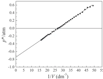
Figure 2 shows the p* vs. 1/V plot obtained for the positive and negative relative pressures. A very good straight line (r2 = 0.9995) was obtained yielding a linear coefficient at 1/V = 0 of (0.749 ± 0.004) atm (see equation 14). Therefore, according to the graphical method, the atmospheric pressure can be obtained with good precision: patm = (0.749 ± 0.004) atm.
The physical chemistry laboratory at the UFVJM, located in the city of Diamantina (State of Minas Gerais, Brazil), is at 1350 m above sea level. The laboratory atmospheric pressure was measured to be 0.773 atm on the same day using a Torricelli’s barometer. Therefore, the relative error (R.E.) obtained with the proposed graphical method is R.E. (%) = [(0.773 − 0.749)/0.773] × 100 = 3.1 %. This small error demonstrates that the graphical method used in this work can be used to measure atmospheric pressure with a simple experimental apparatus.
The number of moles of air present in the apparatus (see Figure 1) can be evaluated from the slope of the line in Figure 2 (see equation 14):
nRT = slope = 0.02778 atm dm3 (17)
Therefore, with R = 0.08205 atm dm3 mol−1 K−1 and T =297 K, one obtains that n = 1.14 × 10⁻³ moles. Given the average molar mass of air1-3 of 28.97 g mol−1, one can estimate a value of 3.3 × 10⁻² g for the mass of the air.
Graphical analysis of pressure-volume data obtained under isothermal conditions: A comprehensive verification of Boyle’s law
After determination of patm using the aforementioned method, a rectangular hyperbola (p vs. V = k(T,n)) was obtained using equation (13) (see Figure 3).
It is worth mentioning that using water instead of mercury did not yield the characteristic hyperbolic behavior (data not shown). In fact, the small change in pressure caused by small increments in the fluid column (water) did not permit to distinguish a rectangular hyperbola from a straight line with a negative slope.19,20
Figure 2. Dependence of relative pressure (p*) of the confined gas on the
inverse of volume. Conditions: V0 = 37.5 cm3 at p* = 0 and T = 297 K
Obviously, simple visual inspection of experimental findings shown in Figure 3 is not sufficient to detect deviations from Boyle’s law. In addition, visual analysis of findings does not allow identification of systematic errors due to using an incorrect atmospheric pressure. Based on these considerations, other linearized plots must be used to assess the precision and accuracy of experimental findings.
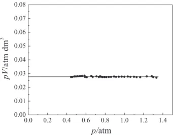
The first rigorous graphical test to verify Boyle’s law is derived from analysis of the product of pressure and volume (p × V) expressed as a function of pressure (p). The resulting (p × V) vs. p plot should yield a horizontal line to support Boyle’s law (see Figure 4). In fact, the analysis of experimental findings showed that the pV product was obtained with good precision: pV = k = (277.8 ± 3.0) × 10−4 atm dm3.This verifies Boyle’s law for the considered pressure range. In addition, point scatter around the horizontal line was minimal. Therefore, the experimental apparatus (see Figure 1) produced experimental results suitable for verifying Boyle’s law.
Another graphical treatment is based on linearization of Boyle’s law (see equation 8), where the p vs. 1/V plot must be a straight line with a positive slope that passes through the origin (see Figure 5). It is worth mentioning that according to equation (8) existence of a non-negligible linear coefficient in the p vs. 1/V plot indicates that the atmospheric pressure used is incorrect (pgas ≠ p* + patm), causing
a systematic error in the total pressure (pgas). Therefore, this graphical analysis provides a means of verifying: (i) the quality (precision) of the pressure-volume data, and (ii) the presence of a systematic error caused by use of an incorrect local atmospheric pressure value. Linear regression analysis yielded the following relationship:
(18)
Analysis of equation (18) shows that the atmospheric pressure obtained using the graphical method presented in Figure 2 was accurate, since the linear coefficient (5.21 × 10⁻⁴ atm) is very small. That is, deviation from the hyperbolic behavior predicted by Boyle’s law is negligible. In addition, a good correlation coefficient was obtained (r2 = 0.9989) which supports the high quality (precision) of experimental results.
The last graphical test used the pVγ = k(T,n) function which
was linearized using the logarithm properties (see equation (9)).19,20 Since the dimensionless parameter (γ) represents the deviations from Boyle’s model, it was assumed in this case that pressure was measured more accurately than volume. In fact, h-values measured in the mercury manometer are more precise than volume measurements with the syringes.
Figure 6 shows the linear plot obtained using equation (9). As can be seen, a good linear behavior was verified. Linear regression analysis yielded the following equation:
ln(p / atm) = –3.561 – 0.993ln(V / dm3) (19) The very good correlation coefficient (r2 = 0.9994) obtained in this case, in conjunction with a γ-value of 0.993, supports the validity of Boyle’s law.
Rationalization of the experiment proposed for verifying Boyle’s law and determining the local (laboratory) atmospheric pressure
Analysis of pressure-volume data obtained with simple analogic instruments using linear models (linearized equations) can clearly aid undergraduate physical chemistry students in several different ways. Important concepts such as the precision associated with measuring a physical quantity using classical (analogic) instruments, the importance of linear regression, as well as use of a graphical method Figure 4. Dependence of the product pV on p. Conditions: V0 = 37.5 cm3 at
p* = 0 and T = 297 K
Figure 3. Hyperbolic behavior of pressure-volume data (p = patm + p*).
Conditions: V0 = 37.5 cm3 at p* = 0 and T = 297 K
to test a theory are presented from a pedagogical perspective during the study of Boyle’s law using a simple and inexpensive experimental apparatus. In addition, students carry out an alternative experiment proposed for determining atmospheric pressure in the laboratory. It is worth mentioning that the study of the fundamental properties of ideal gases using a simple apparatus containing only analogic instruments that can be handled by students themselves is an effective method for teaching several important concepts related to physics, chemistry, and mathematics.
CONCLUSIONS
A brief review of relevant historical aspects of ideal gases was presented. After a critical discussion of Boyle’s law using the pressure-volume data obtained in the physical chemistry laboratory, a graphical method was proposed for determining atmospheric pressure in the laboratory using a simple apparatus composed of a commercial hypodermic plastic syringe connected to a mercury manometer (U-tube). In addition, the analysis of pressure-volume data, obtained at constant temperature, was presented and discussed to emphasize the importance of mathematics and statistics for students in undergraduate physical chemistry courses. Graphical methods using commercial software (Origin 8.0) were presented for students to test Boyle’s law.
ACKNOWLEDGMENTS
L.M. Da Silva wishes to thank the “Conselho Nacional de Desenvolvimento Científico e Tecnológico – CNPq” (PQ-2 grant). Fruitful discussions with my undergraduate students that have occurred over the last 9 years in the classroom and in the physical chemistry laboratory at the UFVJM motivated writing the present work. Therefore, I (L.M. Da Silva), express my sincere gratitude to all of them.
REFERENCES
1. Partington, J. R.; An Advanced Treatise On Physical Chemistry, Vol. 1, Longmans: New York, 1949.
2. Glasstone, S.; Textbook of Physical Chemistry, 2nd ed., Van Nostrand:
New York, 1946.
3. Getman, F. H.; Outlines of Theoretical Chemistry, Wiley & Sons: New York, 1922.
4. Daniels, F.; Outlines of Physical Chemistry, Wiley & Sons: New York, 1948.
5. Moore, W. J.; Physical Chemistry, 4th ed., Prentice-Hall: New Jersey,
1972.
6. Castellan, G. W.; Physical Chemistry, 3rd ed., Addison-Wesley:
Massachusetts, 1983.
7. Levine, I. N.; Physical Chemistry, 5th ed., McGraw-Hill: New York,
2003.
8. McQuarrie, D. A.; Simon, J. D.; Physical Chemistry – A Molecular Approach, University Science Books: Sausalito, 1997.
9. Rosenberg, R. M.; Principles of Physical Chemistry, Oxford University Press: Oxford, 1977.
10. Silbey, R. J.; Alberty, R. A.; Bawendi, M. G.; Physical Chemistry, 4th
ed., Wiley & Sons: New York, 2005.
11. Atkins, P.; de Paula, J.; Physical Chemistry, 7th ed., Freeman: New York,
2002.
12. Laidler, K. J.; Meiser, J. H.; Physical Chemistry, 3rd ed., Houghton
Mifflin: Boston, 1999.
13. Neville, R. G.; J. Chem. Educ. 1962, 39, 356.
14. Laidler, K. J.; The World of Physical Chemistry, Oxford University Press: New York, 2001.
15. Maar, J. H.; História da Química – Primeira Parte, 2nd ed., Conceito
Editorial: São José, 2008.
16. Horstmann, A. F.; Ann. Chem. 1873, 170, 192. 17. Roseman, R.; Katzoff, S.; J. Chem. Educ. 1934, 11, 350.
18. Bosch, W. L.; Crawford, C. M.; Gensler, W. J.; Haim, A.; Levine, I. N.; Linde, P. F.; Salzsieder, J. C.; Silberszyc, W.; Viehland L. A.; Waser, J.; J. Chem. Educ. 1980, 57, 201.
19. Spiridonov, V. P.; Lopatkin, A. A.; Tratamiento Matematico de Datos Físico-Químicos, MIR Publisher: Moscou, 1973.
20. Rangel, R. N.; Práticas de Físico-Química, 3rd ed., Edgar Blücher: São
Paulo, 2006.
21. Slowinski, E. J.; Wolsey, W. C.; Masterton, W. L.; Chemical Principles in the Laboratory, 8th ed., Thomson Learning: New York, 2005.
22. Bettelheim, F. A.; Experimental Physical Chemistry, Saunders Company: London, 1971.
23. Halpern, A. M.; McBane, G. C.; Experimental Physical Chemistry – A Laboratory Textbook, 3rd ed., Freeman: New York, 2006.
24. Steinbach, O. F.; King, C. V.; Experiments in Physical Chemistry, American Book Company: New York, 1950.
25. Daniels, F.; Mathews, J. H.; Williams, J. W.; Bender, P.; Alberty, R. A.; Experimental Physical Chemistry, 6th ed., Book Company: New York,
1962.
26. Weiss, G. S.; Greco, T. G.; Rickard, L. H.; Experiments in General Chemistry – Principles and Modern Applications, 7th ed., Prentice-Hall:
London, 1997.
27. Garland, C. W.; Nibler, J. W.; Shoemaker, D. P.; Experiments in Physical Chemistry, 8th ed., McGraw-Hill: New York, 2009.
28. Davenport, D. A.; J. Chem. Educ. 1962, 39, 252. 29. Davenport, D. A.; J. Chem. Educ. 1979, 56, 322. 30. Miller, D. W.; J. Chem. Educ. 1977, 54, 245. 31. Hermens, R. A.; J. Chem. Educ. 1983, 60, 764. 32. Lewis, D. L.; J. Chem. Educ. 1997, 74, 209.
33. Hays, E. E.; Gustavson, R. G.; J. Chem. Educ. 1939, 16, 115. 34. Suder, R.; J. Chem. Educ. 1983, 60, 735.
35. Blanco, L. H.; Romero, C. M.; J. Chem. Educ. 1995, 72, 933. 36. Torge, W.; Geodesy, 3rd ed., Walter de Gruyter: Berlin, 2001.
Figure 6. Linear behavior of ln(p) vs. ln(V) plot. Conditions: V0 = 37.5 cm3
at p* = 0 and T = 297 K