Automated model selection with applications to
Brazilian Industrial Production index
∗
Jordano Vieira Rocha
†Pedro L. Valls Pereira
‡October 23, 2019
dateSeptember, 2019
Abstract
Brazilian Industrial Production Index undergoes different methodological updates and periods of high inflation over time, which prompts researchers to avoid using too long industrial production series. We analyze how performance of different models in forecasting the Brazilian Industrial Production Index one-step ahead is influenced by the use of samples of different lengths. Relative performance of these models is also assessed. Results show that most models benefit from expanding the estimation sample beginning at least up to 1993:12. Autometrics lag selection with impulse dummy saturation forecasting performance is improved almost monotonically with sample size. For estimation starting in January 1975 and 1985, predictions from Autometrics with impulse dummy saturation and the average of forecasts are statistically more accurate than those from the benchmark AR model. However, the average of predictions performs better in the first half of the forecast horizon and Autometrics performs better in the second half.
Keywords: industrial production index, nonlinear methods, lag selection, dummy
saturation, forecasting.
JEL Classification: C22, C52, C53.
1 Introduction
Macroeconomic data are an indispensable input to policy makers and private agents in cap- turing the economic situation of an entire country or region. They are intended to translate a complex set of heterogeneous variables into informative simple statistics. Since collecting information on all economic agents is unfeasible, macroeconomic data are usually originated from periodic surveys and a limited number of administrative records.
∗The first author acknowledges financial suppport form CAPES and IBGE and second author from CNPq
(309158/2016-8) and FAPESP (2013/22930-0).
†IBGE
Given technological advances and changes in the structure of the economy, the methodol- ogy of such surveys are updated over time. Therefore, using long macroeconomic series may be problematic, specially in forecasting, since recent and old data may be of different quali- ties. Additionally, old data may contain information that is no longer relevant in forecasting future values (this is a characteristic not only of macroeconomic data, but of socioeconomic time series in general).
To investigate the effects of sample size for forecast performance, we analyze the Brazilian industrial production series. The main index of industrial production in Brazil is the Monthly Industrial Survey - Physical Production (PIM-PF), produced by the Brazilian Institute of Geography and Statistics (IBGE). This is one of the longest monthly macroeconomic time series for Brazil, with initial observations in 1975. It is widely used as a business cycle indicator, since the GDP is disclosed quarterly, while the PIM-PF is a monthly index.
Although, in its essence, the index is practically the same over the years — a weighted average of relative quantities, developed over a Laspeyres quantum index — this series has
undergone methodological benchmark revisions over time, which consisted, basically, in up- dating the weights for products and activities, the surveyed set of products and respondents, the level of regional disaggregation, and the industry activity and product classifications, following revisions in international standards.
The last benchmark revision was made in March 2014, which produced revised values up to January 2002. This current series may be insufficiently large, particularly when a fraction of the sample is used for forecast evaluation. On the other hand, as stated before, larger series may contain irrelevant information, suffer from the different methodologies and from the presence of outliers, which may harm parameter estimation. Furthermore, since weights for activities composing the index are fixed for each methodological benchmark, periods of high inflation tend to have distorting influence over the series, possibly generating additional noise.
One objective of this paper is to study the effect of the sample size selection in the forecast performance. Given the intrinsic volatile behavior of industrial production and the structural breaks that may arise also due to changes in the survey methodology, a second objective is to evaluate different linear and nonlinear models, comparing relative performance between them using different sample sizes. We consider only univariate models to rule out the influence of other variables in the analysis.
It is a standard assumption that economic time series are realizations of stochastic pro- cesses, represented by a Data Generating Process (DGP)1. The DGP (or at least a close
approximation) is assumed to be known and any abnormal shift, departing from the stan- dard linear dynamics, in the series must be captured by its form.
Nonlinear models use different techniques to capture these kind of break in a series over time. Some of the most known are composed by a set of different linear models that are al- ternated in time according to some rule of transition. It is the case of the Markov Switching Autoregressive Model (MSAR), which have a transition rule based on a probabilistic struc-
1Some authors consider that the DGP represents the joint density, not necessarily with constant parame-
ters, of all variables characterizing an economy. Following the Theory of Reduction (Hendry, 1995), a subset of these variables can be represented by a Local Data Generating Process (LDGP). To properly parametrize any time-varying effect, an econometric model, usually different from the LDGP, must be a function with constant parameters. See, for example, Bontemps and Mizon (2003).
ture, and the Smooth Transition Autoregressive Model (STAR), with a changing rule based on a transition function that depends on the value of the variable of interest. STAR tran- sitions tend to be more abrupt than those of MSAR, because, in the latter, the transitions are ruled by a Markov Process. This process is characterized by a transition matrix which give the probabilities of switching between regimes, and this characterizes the smoothness of transitions. Early examples of MSAR and STAR models application can be found in Engel (1994) and Teräsvirta and Anderson (1992), analyzing the the US dollar exchange rate and the quarter industrial production indexes from several countries, respectively.
Another way to capture nonlinearities, without explicitly modelling their behavior, is to automatically detect outliers and level shifts, using impulse and step dummies in the model. Santos et al. (2008) propose this approach, selecting the relevant dummies based on the Autometrics algorithm of variable selection (Doornik, 2009). Correctly modeled impulse and step dummies can improve parameter estimation and detect a change in the series’ mean, modifying the conditional mean and avoiding repeatedly wrong forecasts, which would tend to be biased towards the previous unconditional mean. Hendry and Mizon (2011), for example, study the food expenditure in United States using this technique.
However, econometric models may still fail in the presence of unpredictable structural breaks (or changes in the underlying stochastic process). Such fact have been gaining more attention specially after the subprime financial crisis. Abrupt changes in the dynamic of several economic and financial series have caused a phenomenon called forecast failure (e.g.,
Hendry, 2012), i.e., persistent failures in the forecasts after a certain period.
Defining robust forecasting mechanisms, even in the presence of structural breaks of unknown form, becomes important in a world with abrupt, unpredictable events. Hendry (2006) suggests that to predict using the difference of a series (even a stationary one) would make its forecast robust. In the moment of a structural break occurrence, the forecast would be biased, since this change would be unpredictable by definition. In the following periods, however, the forecast would become unbiased, although at the cost of a higher forecast error variance in times of economic stability.
Besides the aforementioned methods, we analyze forecasts from models selecting lags of the dependent variable: the benchmark Autoregressive Model of order p (chosen by the Bayesian Information Criterion), against which all other forecasts will be compared, the Autometrics algorithm without any dummy saturation, and the Least Absolute Shrinkage and Selection Operator (LASSO) and two of its variants, the Adaptive LASSO (AdaLASSO) and the Weighted Lag Adaptive LASSO (WLAdaLASSO), well known regularization and variable selection methods (Tibshirani, 1996; Zou, 2006; Konzen and Ziegelmann, 2016). The simple average of forecasts from all models are also computed.
We perform Diebold and Mariano (1995) test to assess the relative forecast performance using different sample sizes in relation to the current smaller sample (starting in January 2002) for each method. We also test, for each sample, if these methods’ forecasts are more accurate than the benchmark AR(p) model within each sample. Forecasts are made one- step ahead, re-estimating and re-specifying the models at each step. Results show that most models benefit from enlarging the estimation sample at least to 1993:12 and that a rolling window forecasting scheme with this same initial sample performs worse than its expanding window analogous, pointing that information in that period may remain relevant in forecasting future values.
In addition to this introduction, this paper is structured as follows. Section 2 contains an overview of the PIM-PF and the nature of its methodological revisions, Section 3 provides a theoretical review of the considered models, Section 4 details the data used and the settings of the forecasting exercise performed, Section 5 presents the results, Section 6 contains the concluding remarks.
2 An Overview of the Monthly Industrial Survey and its
Methodological Revisions
The Monthly Industrial Survey is part of an integrated system of business surveys2, consisting
of annual (or structural) and monthly (or conjunctural) surveys — the annual and monthly surveys of Mining and Manufacturing (PIA and PIM-PF), of Trade (PAC and PMC), and of Services (PAS and PMS) and the annual survey of Construction (PAIC). There are, ad- ditionally, satellite (or special) surveys, with specific themes, for example, the Innovation Survey (formerly Industrial Survey of Technological Innovation, or PINTEC).
This system is constructed over a unified business register, named Central Business Reg- ister (CEMPRE), which was built in the major revision of business surveys carried out in the mid 1990s. The CEMPRE consists of data and industry classifications of all formal enter- prises and their local units, i.e., all units registered in the Internal Revenue Service, identified
by a unique National Register of Juridical Person (CNPJ) number. It is used to construct the samples of the annual surveys, which, in turn, serve as a basis to calculate the weights and extract the samples of monthly surveys.
Regarding the PIM-PF, the selection of products and respondents of the survey is based on a panel of units representing a percentage of the Industrial Transformation Value (VTI) or the Gross Value of Industrial Production (VBPI) on a base year. In the current benchmark, for example, in each region, only those activities representing 80% of the VTI are surveyed. Of those activities, only the products representing 80% of the VBPI are selected. The local units responsible for 70% of production for each product are surveyed. These fractions are relative to the base year of 2010.
The methodological revisions must be performed periodically to update the set of products and respondents surveyed, the activities analyzed, the industrial classifications, the weighting structure, based on more timely information from economic censuses or annual surveys, and the disagreggation of the index in terms of geographical regions. Seasonal adjustment procedures are also updated as new methodological techniques are developed and suggested by international standards.
The index per se is basically the same, simply a weighted average of relative quantities,
developed over a Laspeyres quantum index:
2This section is based on IBGE’s methodological reports (IBGE, 1991, 1996, 2004, 2015b), on information
from PIM-PF monthly publications and IBGE’s metadata website — available, respectively, at https:// metadados.ibge.gov.br and at https://biblioteca.ibge.gov.br/index.php/biblioteca-catalogo? view=detalhes&id=7228 — and on Góes (2005).
t q q i qi − − t i i i=1 i i i i 0 i i 0 i i 1 i i qt−1 i qt−1
and product panels from months t− 1 and t. Note that
∗ qt != t i 1 i i i=1 i 0 I0 = 0 i i=1 t i , (1) i
where I0 is the index in time t relative to the base year 0, w0 = (V TI0/ n V TI0), and
current series)4.
The first statistics of industrial physical production in Brazil were made in the early 1970s. Initially, the survey included 110 products and around 1000 respondents, using weights from the then recently developed Annual Industrial Survey of 1968. The first reformulation was made with the 1970 economic census publication, available in 1975, which included 600 products and 2500 respondents.
The following update in the series used weights from the 1978 PIA and information from the 1980 Industrial Census, including 736 products and 5000 respondents. With the 1985 Industrial Census (the last economic census to be carried out), the new PIM-PF structure comprised 944 products and 6200 respondents.
The economic statistics system described in the beginning of this section started to be implemented in the mid 1990s. Before this framework, the Industrial Census worked both as a register and provided information for the weighting structure and selection of product and respondent samples, with additional information from the Annual Surveys. The register based on the censuses was rapidly out of date, due to the lag which the census results were available, aggravated by the high rates of birth and deaths of enterprises. The CEMPRE, which is updated each year with administrative data and results from the most recent sur- veys, was developed to overcome those difficulties. Other important technical changes were the use of a new industrial classification system of activities, the National Classification of Economic Activities (CNAE — IBGE, 2003), and of products (PRODLIST-Indústria), and the redefinition of the statistical unit of investigation, from establishment to local unit5.
These changes were incorporated in the PIM-PF only in 2004, covering data from January 2002, which used information from the 1998-2000 editions of the PIA, including 830 products and 3700 local units. The last methodological revision, made in 2015, covering data starting from January 2012, implemented the changes to make the survey compatible with second version of CNAE (IBGE, 2015a). It selected 944 products and 7800 local units.
3The relative quantities are actually calculated as qt
= ( q1 (∗ . ( q2 (∗ . . . ( qt (∗ , where ( qt (∗ is the
relative quantity between months t and t − 1 of produc(t i, m(aintaining the same intersection of respondent
t 1. This adjustment is done to account for this fact, ensuring that relatives are calculated in compatible
panels. 4
In some editions, the weights are calculated over the Value Added instead of the Industrial Transformation Value, i.e., w0 = (V A0/ n
V A0), such as in the series that use weights from the 1985 Industrial Census.
The establishment is defined as an enterprise or part of enterprise that, in a given location, independently engages predominantly in one economic activity. Thus one enterprise may have multiple establishments. The local unit is defined as a physical space where one or more economic activities are developed, corresponding to a unique CNPJ (14 digits) number. The use of establishment as statistical unit revealed problematic, since respondent had difficulties filling out questionnaires and it brought additional complexity in the collecting and
n
qt/q0 is the quantity3 of product i in time t relative to the base period 0 (e.g., 2012 in the
i i 5 w q q q q t i
{I } I t I t K t=1 b1 b1 b1 t t=k2 t=1 1 2 k 2−1 k2 k2+1 K
2.1 The Chaining of Series from Different Methodological Bench-
marks
Each methodological update also changes the base year, i.e., the year in which the average
of the index is 100. This results in multiple series with different levels. For the sake of the series continuity, if we want to obtain a longer time length containing all available data, the entire period must be expressed in the same base.
IBGE’s last technical report (IBGE, 2015b) describe how to link two consecutive series with different base periods. Although this is done to the series of all economic activities that compose the index, we made this procedure only to the General Index, since we do not work with disaggregated data.
Suppose we want to build a series {It}K of an index. Let b1 = (kJan, kFeb, . . . , kDec) and
b2 = (kJan, kFeb, . . . , kDec) be the sets of months composing two different base years. Suppose
b2 b2 b2
that we have two different monthly series of the index expressed in the base years b1 and b2,
b1 k1 and {Ib2 }K , k
2 < k1, and that b2 ⊆ (k2, k2 + 1, . . . , k1). This states that, to make
the link between the series possible, both series must have observations in a given base year. The definition of base year implies that
t∈b1 12 b1 ≡ 100 and t∈b2 12 b2 ≡ 100. (2)
The index of base b1 expressed in base b2 is given by
Ib1 |b2 = Ib1 . t∈b 2 b2 t . (3) Note that t t b1 t∈b2 t t∈b2I b1|b2 = b1 t∈b2 t . t∈b2 I b2 = 100. (4) 12 12 b1 t∈b2 t
The entire series can be, thus, expressed in terms of b2:
{It} ≡ Ib1 |b2 , Ib1 |b2 , . . . , Ib1 |b2 , Ib2 , Ib2 , . . . , Ib2 . (5)
3 Theoretical Review
This section briefly describes the models used in this paper to forecast the Brazilian Indus- trial Production Index series. In following sections, forecast performance of these techniques will be compared to the benchmark Autoregressive Model of order p. We consider non- linear methods (the Markov Switching and Smooth Transition Autoregressive Models), an automatic lag selection and outlier detection method (Autometrics), a naive method robust
t I I I I t=1 t t
to structural breaks (Double Difference Device), and Lasso-type penalty methods (LASSO, Adaptive LASSO and Weighted Lag Adaptive LASSO).
{ } | st ∼ N N f (yt|st = j, θ) = √ 2πσ exp t 2σ2 t f (y , θ) = p(y , s = j, θ) = √ j t st t t+1 t t
3.1 Markov Switching Autoregressive Model
This technique supposes that the DGP consists in different autoregressive models which alternate between them according to a process represented by a discrete latent variable st =
1, 2, . . . , N , in which each value represents a different regime. An additional assumption is that st follows a Markov process, i.e., the probability of the realization of state j in the current
period depends only of the realization of the state from the immediately previous period:
P (st = j|st−1 = i, st−2 = k, . . . ) = P (st = j|st−1 = i) = pij. (6)
The set of probabilities of transition pij can be represented, thus, by a transition matrix
P: p11 p21 . . . pN 1 p12 p22 . . . pN2 P = . . . . . (7) p1N p2N . . . pNN
Suppose, for simplicity and without loss of generality, an AR(1) process in which the intercept (cst ) and autoregressive values (φst ) change according to each regime. We can write
this process as:
yt = cst + φst yt−1 + εt, (8)
where we assume that εt NI(0, σ2 ), i.e., the variance of the error term also depends on st.
Observe that, even if we know all the involved parameters, we cannot be sure of which regime the process is in each period. Let θ be the vector containing all the parameters in the model. We can infer the state by the probability that the process is in regime j conditional to the realization of the series values up to t, denoted P (st = j yt, θ). Following the law of
conditional probabilities:
P (s = j|y , θ) = p(yt, st = j, θ) = πjf (yt|st = j, θ) . (9)
f (yt, θ) f (yt, θ)
In the expression above, πj = P (st = j, θ) is the unconditional probability of st assuming
the value j, f (yt|st = j, θ) is the conditional density, assumed normal, that is:
1 { −(yt − cs − φs yt−1)2
st st
and the unconditional density is given by:
π { −(y − c − φ y )2
Stacking the conditional densities f (yt|st = j, θ), the conditional probabilities P (st =
j|yt, θ) and the forecasts P (st+1 = j|yt, θ) in vectors (N × 1), respectively, ηt, ξˆ|t e ξˆ |t, i.e.,
t t t j=1 j=1 st . . 2σ (10) exp st t−1 . (11) 2πσ 2 st
. . .. t × t 1 t|t − − | t f (yt|st = 1, yt−1; θ) η = f (yt|st = 2, yt−1; θ) f (yt|st = N, yt−1; θ) P (st = 1|yt, θ) P (st = 2|yt, θ) (12) (13) t|t ξˆ . P (st = N|yt, θ) P (st+1 = 1|yt, θ) = P (st+1 = 2|yt, θ) . (14) t+1|t P (st+1 = N|yt, θ)
Hamilton (1994) shows that the optimal inference for the regimes is given by the following recursion: ξˆ = (ξˆ|t−1 ηt) (15) t|t ˆ t|t−1 ηt) ˆ t+1|t ˆ t|t , (16)
where P is defined by (7), represents element-by-element multiplication and 1 is a (N 1) vector of 1’s.
The likelihood maximization problem is given, thus, by:
T T max L(θ) = f (yt|yt−1, θ) = 1l(ξˆ|t−1 ηt) (17) t=1 t=1 s.t. (pi1 + pi2 + · · · + piN ) = 1, pij ≥ 0, ∀j, i. (18)
Expression (15) is similar to (9), and (17) similar to (11).
Given the values of θ0 and ξˆ |0 (e.g. ˆ 1|0 = ρ, with ρ = 1/N ), the recursion in (15)-(16)
returns the values of ξˆ . Note that, for each t, this method utilizes only the realized values in the current and in previous periods (t, t 1, t 2, . . . ) in order to estimate P (st = j yt−1, θ).
However, we possess additional information to increase this estimate’s accuracy, namely, the remainder of the sample (t + 1, t + 2, . . . , T ). For this, we have to use a smoothed inference
=
l1 (ξ
ξ = P ξ
ξ ξˆ
11
|
Let us denote, generalizing the previous notation, the probability of being in a regime conditional to the realized values from the series and to the parameters P (st = j yτ , θ). For
t < τ , we will have a smoothed inference of regime t. Kim (1994) develops a recursion
T |T T −1|T 1|T t|t | Y Y | Y { ˆ t|T ˆ t|t { Pl[ξˆ ˆ t+1|t , (19)
where (÷) means term-by-term division.
The iteration algorithm starts in ξˆ , which, in turn, is calculated from (15)-(16), passing through ξˆ ˆ T −2|T , . . . , ξˆ . Once having ξˆ ˆ t+1|t known, the full vector of maximum
likelihood estimates θˆ is obtained solving (17)-(18), proceeding recursively until there is convergence to a θ∗. Restricting pij ≥ 0 and pi1 + pi2 + · · · + piN = 1 for all i, j, and supposing
ˆ
1|0 is fixed and not related to the other parameters, Hamilton (1990) demonstrate the the
transition probabilities estimators pij are given by:
pˆ = T t=2 P (st=j, st−1 = i|yT , θˆ) , (20)
ij T
t=2 P (s t−1 = i|yT , θˆ)
that is the sum of the probabilities of regime i being followed by regime j divided by the sum of the probabilities of being in regime i.
Finally, to calculate the optimal forecast one-step ahead, suppose we know which will be the regime in period t+1, so the prediction will be obtained by hjt = E(yt+1 st+1 = j, t; θ) =
yt+1f (yt+1 st+1 = j, t; θ)dyt+1, where t is a vector containing all y observations through
date t. The unconditional expectation will be, thus, given by:
E(yt+1|xt+1, Yt; θ) = yt+1f (yt+1|xt+1, Yt; θ)dyt+1 = yt+1 N j=1 { N p(yt+1, st+1 = j|xt+1, Yt; θ) dyt+1 = yt+1 j=1 [f (yt+1|st+1 = j, xt+1, Yt; θ)P (st+1 = j|xt+1, Yt; θ)] dyt+1 = j=1 N P (st+1 = j|xt+1, Yt; θ) yt+1f (yt+1|st+1 = j, xt+1, Yt; θ)dyt+1 = P (st+1 = j|Yt; θ)E(yt+1|st+1 = j, xt+1, Yt; θ). (21) j=1
If we stack hjt in a vector (N × 1) ht, then:
ξ = ξ t+1|T (÷)ξ , ξ and ξ ξ N
13
Y
t+1
Although the Markov Chain admits a linear representation, the optimal forecast one-step ahead is a nonlinear function of the of the observed variables, for ξt|t depends on t in a
nonlinear way. As pointed by Hamilton (1994), this implies that, if, inside a regime, an outlier (an observation little likely to be generated in this regime) is observed, the framework analyzed here has high probability of inferring that a change of state has occurred.
∼
→ ∞
j=1
3.2 Smooth Transition Autoregressive Model
As it is the case with MSAR models, the STAR models consist in two or more regimes following different linear autoregressive processes. The transition dynamics from one regime to another is, though, different. The change between states is given by a transition function as described below.
Suppose a stochastic process represented by the following DGP:
yt = π10 + π1l zt + (π20 + π2l zt)F (yt−d) + t. (23)
F (yt−d) is called the transition function, it depends on the model’s dependent variable,
yt, lagged by the parameter d, that will be estimated. The vector zt = (yt−1, yt−2, . . . , yt−p)
contains the lagged series, (π1, π2) are parameter vectors with correspondent dimensions and
(π10, π20) are scalars. The error term is assumed normal, independent and identically dis-
tributed, i.e., t NI(0, σ2). It is important to stress that t is symmetric, so that rejections of
the null hypothesis from linearity tests would come from the model parametrization, and not from the error term.
The F function is limited between 0 and 1. In case it is an indicator function F (yt−d) =
I(yt−d > c)6, the model is denoted Self Exciting Threshold Autoregressive (SETAR), in which,
when yt−d is greater than the threshold c, the regime is changed instantaneously. To establish
a smooth transition between the regimes, we can use some continuous function between 0 and 1, so that the parameters of (23) vary, as function of yt−d, between π10 and (π10 + π20)
for the intercept, and between π1 and (π1 + π2), for the autoregressive parameters. These
values correspond to the two extreme regimes (F = 0 and F = 1, respectively). There are two functions used predominantly in the literature. The first is the logistic function:
F (yt−d) = (1 + exp[−γ(yt−d − c)])−1. (24)
When the model uses the function above, it is called Logistic Smooth Transition Autore- gressive (LSTAR). The inclination parameter γ measures the speed of transition from one
regime to another, and the location parameter c is the threshold. Besides, when γ , the model approximates a SETAR model.
LSTAR model has been used to model macroeconomic series with asymmetric behavior. Öcal and Osborn (2000) and Teräsvirta and Anderson (1992) use it to model industrial production series and Skalin and Teräsvirta (2002) for unemployment series.
The second function is the exponential function:
F (yt−d) = 1 − exp(−γ(yt−d − c)2). (25)
Using this function, we denote the model Exponential Smooth Transition Autoregressive (ESTAR). The interpretation given to the parameters γ and c is the same as in LSTAR. When γ → ∞, however, F tends to I(yt−d = c).
6We will use, in this work, only two regimes, corresponding in theory to periods of expansion and periods
of recession, but we could generalize for more regimes. In this case, the model would have, in the indicator function example, the form yt = r α ztI(cj−1 < yt−d < cj) + t, with cj representing each threshold.
|
t− t−
The ESTAR model is normally used in series with symmetric behavior. In this case, we would have one regime when yt−d gets near the threshold and another when it gets far. An
example of application is Arango and Gonzalez (2001), who models the Colombian inflation acceleration.
To verify if there are gains in formulating a nonlinear specification, we should do a linearity test. Besides, we will need this test to estimate the parameter d. There is, however, a caveat in performing this test, for there are many ways of defining linearity in (23)-(24)/(25).
When we test H01 : γ = 0 in (23)-(24), the model will be identified only under the
alternative hypothesis, because π20 and π2 will be able to assume any value. If, on the other
side, we test H01 : π20, π2 = 0, γ and c will be able to assume any value. A similar reasoning
applies to (23)-(25).
To contour this problem, Teräsvirta (1994), based on Davies (1977) and on Luukkonen et al. (1988), elaborates a test from a Taylor expansion around γ = 0, leading to the following auxiliary regression: p p p uˆt = wˆ1 l tβ˜1 + β2j yt−j yt−d + β3j yt−j y2 d + β4j yt−j y3 d + vtl , (26)
where uˆt are the residuals from the (linear) AR(p) model estimation,
β˜1 = (β10, β1
l
)l. The null hypothesis of linearity is:
wˆ1l t = −(1, ztl)l and
H0
l
: β2j = β3j = β4j = 0, j = 1, . . . , p. (27)
Each βij is a combination of the parameters from (23), different, thus, for (24) and (25).
Comparing these combinations, (26) will have different formats and Teräsvirta (1994) elaborates successive F-tests which can distinguish between on function and another. They are7: 1. H0 l 1 : β4 = 0. 2. H0l 2 : β3 = 0|β4 = 0. 3. H0 l 3 : β2 = 0|β3 = β4 = 0. If H0 l
1 is rejected, we have evidence in favor of the LSTAR model, otherwise, we can
use the ESTAR model. If H1l 0 and H2l 0 are not rejected, we also have evidence in favor of
LSTAR, the hypothesis rejection, however, is not informative. If the true model is a LSTAR,
H0
l
3 is generally rejected. If H0
l
3 is not rejected and H0
l
2 is rejected, we choose the ESTAR
model. If H0
l
3 and H0
l
2 are not rejected, but H0
l
1 rejected, LSTAR model is selected. The
only inconclusive case is when H0
l
1 and H0
l
2 are rejected. In this situation, we test:
H0 ll 2 : β3 = 0|β2 = β4 = 0. (28) However, if H0 l 2 is rejected, H0 ll
2 should be rejected even more strongly. 7The notation β
i = 0 βj = 0 means that the test βi = 0 is made conditional on the non-rejection of the
previous test βj = 0. Thus, H0 2 is made conditional on the non-rejection of H0 1, and H0 3 is made conditional
on the non-rejection of H0 2 and of H0 1.
|I ≥
Parameter estimation can be done by Nonlinear Least Squares, that, under the assumption of normality, is equivalent to the estimation of Conditional Maximum Likelihood. Under some assumptions and regularity conditions (Wooldridge, 1994), estimators are consistent and asymptotically normal. The estimation procedure is thus carried out with standard numerical algorithms (e.g. Newton-Raphson and BFGS).
This work’s objective is to make one-step ahead forecasts, re-specifying the model at each period. It is, therefore, impracticable and counter-intuitive to decide, at each step, if the DGP comes from a STAR model with logistic function or with an exponential function. Impracticable for the fact that the test explained above for the most appropriate function contains inconclusive situations, making it difficult to construct an algorithm for real-time automatic forecast. Counter-intuitive because the change in the function at each step would imply that, given the information at each new observation, the entire series generating process would be revalued, being governed alternatively by a function characterizing asymmetric series and by a function characterizing symmetric series.
Since, usually, industrial production tends to have an asymmetric behavior, i.e., its growth
dynamics is different from its recession dynamics, we opted to use only the logistic function in the specification of the STAR model.
Castle and Hendry (2014) investigate, through Monte Carlo simulations, the LSTAR models forecast and estimation efficiency for different magnitudes in the transition probability from one regime to another and differences between the intercepts of each regime. They conclude that, for very high γ’s, estimation becomes imprecise. Besides, there must be a large number of observations in each regime. For this to happen in small samples, it would be necessary a large probability of change between regimes. On the other side, the constant change of regimes can imply that the series is better modeled by a linear autoregressive process. These problems tend to be solved in reasonably large samples.
Concerning the forecast results, precision, measured by the Root Mean Squared Forecast Error (RMSFE), of a correctly specified LSTAR with one lag improves considerably in large samples and when the difference in the mean of each regime is not very large nor very small (the cited authors analyze changes of 1, 2, and 5 standard-deviations in the intercept).
From equation (23), the one-step ahead forecast, conditional to the information up to time t (It), is given by:
E[yt+1|It] = E[π10 + π1 l zt+1 + (π20 + π2 l zt+1)F (yt+1−d) + t+1|It] = π10 + π1 l zt+1 + (π20 + π2 l zt+1)F (yt+1−d), (29)
where the terms zt+1 and F (yt+1−d) are values already realized in period t, because zt+1 =
(yt, yt−1, . . . , yt−p−1) and d 1.
More-steps ahead forecasts are more complex, because obtaining E(yt+2 t) is more diffi-
cult and would have to be done by numerical integration. This work, however, makes only one-step ahead predictions, which dismisses a deeper explanation of the subject8.
8See Lundbergh and Teräsvirta (2005) for more detailed reference in forecasting more than one steps
3.3 Autometrics
Autometrics has its origin in the so-called London School of Economics methodology, whose econometric technique is based on a general-to-specific modeling. In this approach, the researcher chooses a reasonably large number of variables which have a theoretical relation with some dependent variable and, from this general model, he performs specification and significance tests to gradually reduce the set of relevant variables.
This methodology opposes to the so called specific-to-general, that is more frequently used by econometrics practitioners. It consists in starting with simple models containing few variables and, according to diagnostic tests results, adding other variables or modifying the used specification.
The algorithm called Autometrics is presented in Doornik (2009). This type of algorithm, however, has its origin in the works of Lovell (1983) and Hoover and Perez (1999). Later, Hendry and Krolzig (1999, 2005) improve previous works, arriving at a structure similar to Autometrics, which has been continuously improved since then.
Hoover and Perez (1999) consider four main characteristics in their selection mechanism. First, the concept of General Unrestricted Model (GUM), that is a linear regression model involving a large number of variables relating with the utilized dependent variable. Second, the use of multiples search paths, where the first path begins with the elimination of the variable with the largest p-value in the significance test, the second path with the elimination of the variable with the second largest p-value and so on until the tenth variable. Third, at each step of each path, it is performed a joint significance test including all the eliminated variables so far in relation to the GUM. Fourth, at each step of each path, a battery of specification tests are also performed.
In Hendry and Krolzig (1999, 2005), the authors improve the existing algorithm, creating the software called PcGets (from general-to-specific). Differently for the previous mechanism,
more paths are followed eliminating sets of variables, and there is a pre-selection of lags before the reduction begins. Besides, each path’s “terminal” — when it is not possible to remove any more variable without failing in some test — are united in a set of variables which will form the new GUM. The algorithm is finished when there is convergence, i.e., the current
GUM equals the previous GUM.
In the end, we will have many candidates which cannot be reduced. Among them, the final candidate is chosen by the minimum Bayesian information criterion (BIC) in Hendry and Krolzig (1999, 2005) and by the best fitted model in Hoover and Perez (1999).
3.3.1 Autometrics’ Selection Algorithm
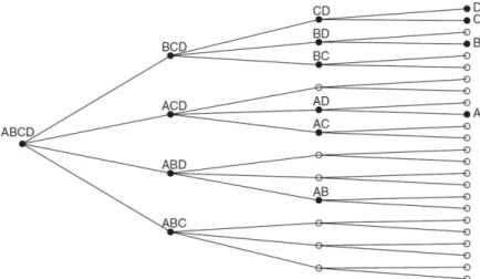
In Doornik (2009), starting with the GUM, the selection mechanism seeks to consider the models with all possible variable combinations. It utilizes a tree representation (Figure 1), in
−
b 2 a a
Figure 1: Tree for Possible Models in Autometrics.
The algorithm runs through the tree, following the nodes from left to right and from top to bottom, so that, in the Figure 1 example, it would pass through the models ABCD, BCD, CD, D, C, BD and so on. In each node, the variables are ordered in crescent order of significance, that is, in the GUM, A is the least significant variable and D is the most significant. It is possible that, in the following node, the order will be changed. For example, if C is less significant than B, the ordering would be given by CBD and the variable to be eliminated would be C.
If all the nodes from the tree were evaluated, the computational cost would be very large (for n regressors, 2n 1 models would be estimated), so a number of strategies to jump the
irrelevant nodes are used. These strategies are classified by Doornik (2009) as Pruning, Bunching, Chopping and Model Contrast.
Pruning consists in ignoring the nodes derived from a node invalidated by a diagnostic test or by backtesting (a joint significance F-test with relation to the initial GUM). If, e.g.,
starting from BCD, variable B cannot be eliminated, models CD, D and C are not estimated. The p-value used is denoted pa.
Bunching stems from the idea that it is possible, instead of eliminating the variables individually based in a t-test, eliminating groups of variables based in a F-test with relation
1/2 3/4
to the current node. The size of the group to be tested is defined by p = max{ 1
p , p }9,
the p-value of the joint significance test. The F-tests significance level for which the group is eliminated, however, is the same as Pruning’s, i.e., pa. Once the group of variables is
eliminated, we get to the correspondent following node, avoiding estimation of many models. In the example of Figure 1, if we are at BCD and are able to effectively eliminate jointly B and C, the next model to be estimated is that containing only D, ignoring CD. If, in group, the variables cannot be withdrawn, we test the removal of groups with less variables, until a valid reduction is achieved.
Chopping means ignoring models, in a given ramification from a node, containing some variable or group of variables if they are of very little significance. For example, if we are, again, in BCD and BC presents a F-test with a greater p-value than a certain pc, the algorithm
will estimate, in this ramification of the tree, only model D and will go next to node ACD. The standard p-value used by Autometrics is pc = pb.
Model Contrasts consist in the elimination or shortening of paths in a certain ramification of the tree if it contains some terminal already found previously, so that it jumps to the nodes possessing possible terminals not yet estimated. As an example, suppose that, in the above Figure, we had selected D as a terminal in the first ramification. In the next step, ACD, the following node, AD, would originate two possible models: A and D. As D was already selected, the algorithm tests directly a reduction of ACD to A, speeding the calculations.
There are two types of Model Contrast: Union Contrast and Terminal Contrast. In the first, used when the current GUM is different from the previous GUM, the program considers, to jump, nodes that lead to any model different from the terminal union. In the second, used when the current GUM equals the previous, the jumped nodes takes into account paths that lead to terminals different from each one of the previously individually found terminals.
Several specification tests are then performed. However, differently from the algorithms cited earlier, in Autometrics they are performed only when the terminals are attained. If some test fail in some terminal, the program follows the path backwards from the node, making specification tests until some valid terminal is found. The tests performed are: residuals normality (Jarque and Bera, 1980), second order residual autocorrelation (χ2 test, Godfrey,
1978; Breusch and Pagan, 1980), autocorrelated conditional heteroscedasticity (ARCH) to second order (Engle, 1982) and that of in-sample stability (Chow, 1960).
In each iteration of the GUM, Autometrics divides the search in two stages. In the first, it ignores paths whose nodes contain terminals. In the second, it follows the root paths which contain terminals, using Model Contrast to reach definitive terminals more quickly.
Furthermore, before initializing the algorithm per se, there is the option of performing a
presearch to eliminate sets of variables or lags. The general model after the presearch is used as the GUM in the algorithm. Several options of lag and variable reduction are available. It is out of the scope of this paper to explain the details of the presearch procedures. For a description of the different options, see Doornik (2009).
Finally, when all the tree paths are covered, the final terminals where specification tests failed are discarded and, after the GUM convergence, i.e., when the previous GUM is equal
to the current GUM, the terminal with the minimum BIC is chosen.
3.3.2 Dummy Saturation
A way to detect discrepant observations (outliers) in the series and other possible nonlinear- ities is the use of impulse dummy variables — which assume value 1 for observation t and 0 for the others — for the periods they occur. Proceeding according to the Gets methodology,
we would have one dummy variable for each observation, besides other exogenous variables which could possibly affect the dependent variable. This framework is denoted as a Dummy Saturation model.
Trying to estimate the GUM this way is obviously impracticable, because there are more variables than observations. Autometrics, however, utilizes a technique to reduct these mod- els, initially proposed by Hendry and Krolzig (2005) and applied to the Impulse Indicator Saturation (IIS) context by Santos et al. (2008).
− j=1 t E E || t
tion mechanism described above only with the T/2 first dummies, so that the resulting model will contain a subset of them. After this, the same is done with only the T/2 last dummies. Thus, we will obtain two models containing subsets of the initial dummies, the union of these models will generate a new GUM. Applying once more the reduction mechanism, we obtain the model containing the relevant dummies.
A generalization of this method can be applied when step dummies — which assume value 0 up to observation t 1 and 1 in the following observations — and other exogenous variables are included in the GUM. In this case, the algorithm introduced by Hendry and Johansen (2012) assumes N = N nj regressors so that N > T and nj < T for all j, that
is, the N regressors are partitioned in portions smaller than the sample size.
Once the best fitted model is found, with relevant variables and dummies, the forecast is made in the standard way, i.e., the model’s n-steps ahead mathematical expectation.
3.4 Double Difference Device
Consider a variable yt that we want to predict10. Suppose yt ∼ Dy (yt|Yt−1, θ), where θ ∈ Θ ⊆
Rk and Yt−1 = (y1, . . . , yt−1). For a sample of size T , a forecast h step ahead is a combination
of the sample values from 1 through T , i.e., yˆT+h|T = fh(YT ). It can be proven (for example
in Clements and Hendry, 1998) that yT +h T = E[yT+h YT ] is the unbiased predictor which
minimizes the Mean Square Forecast Error (MSFE) and holds the minimum variance within the unbiased predictor class.
Suppose yt follows the linear autoregressive process below:
yt = µ + ρyt−1 + γzt + t, with t ∼ IN (0, σ2) e |ρ| < 1, (30)
where {zt} is an exogenous variable, forecast error’s mean and variance are, respectively,
E[yT +1 − yT +1|T ] = 0 and V [(yT+1 − yT +1|T )] = σ2.
Consider E[yt] = θ and zt ∼ N (κ, 1). We can write the mean of yt as:
E[y ] = θ = µ + γκ. (31)
1 − ρ
If µ = κ = 0, a break in ρ will not affect the mean of yt. However, in case that we have one
of these parameters different from zero, a change in the autoregressive parameter will imply a change in the mean. Besides this, if more than one of these parameters suffer a break, the forecast failure can be even more severe. For example, if the autoregressive parameter and the intercept, ρ and µ, are, respectively, 0.8 and 8, and suffer a break, becoming 0.6 and 6, the unconditional expectation shifts from θ = 40 to θ∗ = 15.
Let us rewrite the model (30) as:
10This exposition is based in Hendry (2012), and simplifies the more general theory with multiple variables
− − | ∆y = µ + (ρ − 1)y + γz + + (ρ − 1) µ + γκ − (ρ − 1) µ + γκ t t−1 t t 1 − ρ 1 − ρ = µ − µ − γκ + (ρ − 1)(yt−1 − θ) + γzt + t = (ρ − 1)(yt−1 − θ) + γ(zt − κ) + t.
Rearranging the terms, i steps ahead values can be written as:
∆yT+i = ω + α(yT+i−1 − θ) + γzT+i + T+i, (32)
where ω = γκ and α = ρ 1.
This formulation is denoted Equilibrium Correction Model (EqCM), where the equilib- rium is given by θ. Forecasts will tend to return to θ independently of the behavior of the data. Changes in this equilibrium, which occur mainly by shifts in the level, consist in the main factor which imply forecast failure.
A naive predictor is the called Double Difference Device (DDD). Its intuition comes from the fact that most economic variables do not continuously accelerate and, hence, its second differences have unconditional expectation E[∆2yt] = 0, suggesting the following DDD
estimator:
∆yT +1|T = ∆yT , (33)
where ∆yT +1 T denotes a one-step ahead forecast for ∆yT given the information in time T .
Because the forecast does not utilizes any parameter, structural breaks do not persistently influence it, and the estimator is unbiased.
Let us modify equation (32) so that the DGP does not contain exogenous variables besides the dependent variable lags (i.e. γ = 0):
∆yT+i = α(yT+i−1 − θ) + T+i. (34)
Suppose there is a break in the parameters, so that the DGP becomes:
∆yT+i = α∗(yT+i−1 − θ∗) + T+i. (35)
EqCM forecast error is given by:
∆yT +i − ∆yT +i|T +i−1 = ∆yT +i − αˆ(yT +i−1 − θˆ) + T +i = wT +i, (36)
where the hat over the parameters means that they were estimated on the EqCM formulation. Replacing the in-sample estimated values for the pseudo-true in-sample population values, where E[θˆ] = θp, we can reduce the forecast error variance without damage to the general
analysis. Thus, we have:
E 2
E E E M [uT+i] = 2σE 1 + 2 + α
With respect to the DDD (∆ yT +i|T +i−1 = ∆yT+i−1), for i > 1, we have:
∆yT +i−1 = α∗(yT +i−2 − θ∗) + T +i−1. (38)
The respective forecast error is calculated as:
∆yT +i − ∆yT +i|T +i−1 = uT +i = α∗(yT +i−1 − θ∗) + T +i
− [α∗
(yT +i−2 − θ∗) + T+i−1] (39)
⇒ uT +i = α∗∆yT +i−1 + ∆ T+i. (40)
On the long term, values are replaced by their unconditional expectations, i.e.:
E[uT+i] = α∗E[∆yT+i−1] + E[∆ T+i] = 0 (41)
V [uT+i] = V [α∗∆yT+i−1] + V [∆ T+i]
= α∗2V [∆yT+i−1] + 2σ2. (42)
As it is evident from (40) and (42), the Double Differencing mechanism adds some noise sources by the extra differentiation of α∗yT −i+1 and of T +i. This extra source of noise,
however, can be of lower dimension than those from the traditional autoregressive model when there is presence of structural breaks in the series’ unconditional mean.
To illustrate, suppose that the shift occurs only in µ, so that θ changes and α remains constant. We will have:
wT+i = −α(θ∗ − θ) + T+i E[wT+i] = −α(θ∗ − θ) V [wT+i] = σ2 uT +i = α∆yT +i−1 + ∆ T +i E[uT+i] = 0 V [uT+i] = V [α∆yT+i−1] + V [∆ T+i].
The MSFE is approximately:
M [wT+i] = α2(θ∗ − θ)2 + σ2. (43)
Comparing with the DDD MSFE:
2 α
2
Assuming ρ = 0.8, ∇µ∗ = µ∗ − µ = 0.2, and σE = 0.06, we have α = −0.2 and ∇θ∗ =
θ∗ − θ = 1. With these values, M [wT+i] is approximately 6-fold larger than M [uT+i].
j
xij/N = 0 and x2 /N = 1) to rule out problems of differences in their scales. For
3.5 LASSO and Derived Methods
Developed by Tibshirani (1996), the Least Absolute Shrinkage and Selection Operator (LASSO) is based on a class of estimation procedures known as shrinkage methods, which shrink Ordi- nary Least Squares (OLS) coefficients estimators towards zero. This approach aims to reduce the variance in the bias-variance trade-off, introducing some bias in the estimators.
Consider the data (xi, yi), i = 1, . . . , N , where xi = x
i1, xi2, . . . , xip are the regressors and
yi the dependent variable, and assume that the yis are conditionally independent given the
xijs. The LASSO estimator solves the following problem:
N min α,β yi − α − βj xij 2 , subject to |βj| ≤ t, (45) i=1 j j w
here t ≥ 0 is a t uning parameter. The independent variables are standardized (i.e., all t, the solution for α is given by αˆ = y, so that (45) can be solved omitting the intercept.
The problem can be expressed in its equivalent Lagrangian form:
N min α,β yi − α − βj xij 2 + λ |βj|. (46) i=1 j j
For λ = 0 (for a sufficiently large t), the restriction in (46) is nonbinding and βˆLASSO = βˆ,
the OLS estimator. Higher values of λ impose the estimators a penalty, shrinking them towards zero. Depending on the value of λ, some of the LASSO coefficients are set to be exactly equal to zero, performing, thus, a method of variable selection.
To better understand this characteristic of the LASSO, consider an earlier example of reg- ularization method introduced by Hoerl and Kennard (1970), the Ridge Regression estimator, which solves the following problem (also in its Lagrangian form):
N min α,β i=1 yi − α − βj xij j 2 + λ β2, (47) j
with the same set-up of the LASSO.
The difference between the two methods lies in the form of the penalty: the LASSO uses the L1-norm penalty and the Ridge Regression uses the L2-norm penalty.
Due to the L1-norm used in LASSO, the solution to (46) is nonlinear in yi, for which there
is no closed form expression. For the Ridge Regression, the solution takes the form βˆRIDGE
= (XlX + Iλ)−1Xly. Note that, differently from the LASSO, βˆRIDGE will generally
have all its components different from zero. To see this, consider Figure 2 below.
i i ij
Figure 2: Estimation picture for LASSO (left) and Ridge Regression (right). Source: Tib- shirani (1996).
In a two parameter space, the OLS estimator is represented by βˆ, the ellipses are contour plots for the same sum of squared residuals, and the black area represents the possible values under the constraint for some t. The corners on the restriction area make the LASSO estimator, in the left, to fix one of the coefficients exactly at zero. The Ridge Regression estimator, in the right, shrinks the OLS estimator towards zero, but does not, as a rule, estimate exactly zero coefficients.
Up to this point, our analysis treated λ as given. In practice, we have to choose it according to the data. Probably, the most common approach to estimate λ is by cross- validation, which aims to minimize an estimate of the expected prediction error11. However,
cross-validation may present difficulties in a time-series framework. Zou et al. (2007), Zhang et al. (2010), Wang et al. (2007) argue that using the Bayesian Information Criterion (BIC) is a good alternative to cross-validation in selecting λ. We follow Medeiros and Mendes (2016), Medeiros and Vasconcelos (2016) and Konzen and Ziegelmann (2016), for example, in using the BIC to select the tuning parameter.
3.5.1 AdaLASSO
Fan and Li (2001) defined a procedure satisfying the oracle properties as one that, asymp- totically, selects the correct subset of variables with nonzero coefficients and has an optimal estimation rate. Zou (2006) states that if, for some λ, the LASSO has an optimal estimation rate, then it does not satisfy variable selection consistency. The author also argues that, even relaxing an optimal estimation rate, variable selection is consistent only under a nontrivial condition (similar conclusions were made by Meinshausen and Bühlmann, 2006 and Zhao and Yu, 2006).
Zou (2006) proposed, thus, a slight modification to the LASSO, the Adaptive LASSO (AdaLASSO) estimator, which solves the following problem:
11See Hastie et al. (2009) for a more detailed explanation of the cross-validation method for model selection
| | j j | | ≥ N min α,β yi − α − βj xij 2 + λ wˆj|βj|, (48) i=1 j j
where wˆj = βˆF ST EP −γ , γ > 0, and βˆF ST EP is a first step estimator of β. One can use, for
example, the OLS estimator, the Ridge Regression estimator, or the LASSO estimator (as in Garcia et al. (2017)). We opt to use βˆF ST EP = βˆRIDGE and γ = 1.
The AdaLASSO assigns different penalties to each variable, with higher penalties to variables whose coefficients are closer to zero in the first step estimation. Zou (2006) proves that the AdaLASSO is an oracle procedure.
3.5.2 WLAdaLASSO
Another variant of the LASSO we use is the Weighted Lag Adaptive LASSO (WLAdaLASSO), proposed by Konzen and Ziegelmann (2016), based on the work by Park and Sakaori (2013). This method is similar to the AdaLASSO, and it comes from the observation that, in a time- series autoregression framework, more distant lags tend to have less influence in forecasting the dependent variable, imposing on them higher penalties. The estimator solves:
N min α,β i=1 yi − α − βj xij j 2 + λ wˆW L|βj|, (49) j
where wˆW L = ( βˆRIDGE e−αl)−γ, l is the lag order, and γ > 0, α 0 are tuning parameters.
As in AdaLASSO, we set γ = 1. To select α, for a given λ, we estimate the model considering a grid (0, 0.5, 1, . . . , 10) for α and choose that with the lowest BIC. The parameter λ is then selected considering the model with the lowest BIC (see Konzen and Ziegelmann, 2016 and Prince and Marçal, 2018).
Monte Carlo simulations performed by Konzen and Ziegelmann (2016) pointed that the WLAdaLASSO was superior to both LASSO and AdaLASSO in variable selection, parameter estimation and forecasting, particularly when the candidate variables included a high number of lags and predictors presented stronger linear dependence.
4 Empirical Framework
The objective of this work is twofold. The first is to test if there is any gain in using ex- tended series of Brazilian Industrial Production, the second is to assess if nonlinear univariate methods have better forecasting performance than the autoregressive model.
This section details the PIM-PF time-series available and describes the forecasting exercise we perform. It also details the method to test whether forecasts accuracy are statistically different between models.
4.1 PIM-PF Data
There are, as mentioned in the previous paper, three different series available in IBGE’s System of Automatic Data Retrieval (SIDRA): 1985:01-2004:01, with base year 1991, 1991:01- 2014:02, with base year 2002, and 2002:01-2018:12, with base year 2012. There is an extended version of the first series available in the Time Series Management System (SGS) of Brazilian Central Bank (BCB), ranging from 1975:01 to 2004:01, where the 1985:01-2004:01 values are identical to those from SIDRA.
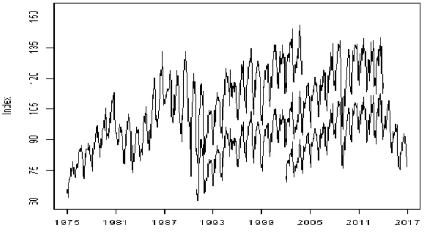
Figure 3 plots the three series in one graph. Note that there is considerable overlap between their covered time span. This is because the closed series published by IBGE already contain chained values from the previous one.
Figure 3: PIM-PF Series Expressed in Different Base Years.
One reason the entire chained series is not always published is that there are difficulties in the chaining components disaggregated by activities, due to changes in the classification system and different list of selected products in each revision. The chaining of the aggregated series is, on the other hand, straightforward and plausible. Figure 4 contains the chained series, constructed as described in (3) and (5), of the General Industrial Production quantum
for whole sample.
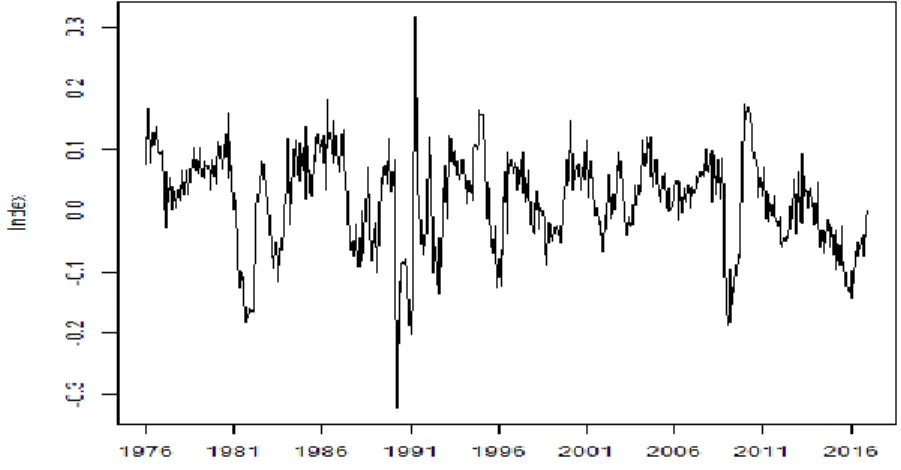
The presence of non-stationarity and seasonality in the series is easily noticed. To deal with these characteristics, the log of the series is differenced with relation to the same month in the previous year. This corrects both problems if the series is integrated of order one and has constant seasonality12. Figure 5 shows a graph with the treated series.
For nonlinear models with different regimes, specification becomes more robust when data shows well defined different regimes. In STAR models, for example, γ estimation becomes difficult if the probability of crossing the threshold c is large, i.e., the regime are not very well
12The presence of stochastic seasonality, however, may not be eliminated with this transformation. In fact,
even standard seasonal adjustment methods may fail to correctly account for stochastic seasonality. The use of Autometrics with dummy saturation, however, can improve the modelling of non-deterministic seasonality.
Figure 4: Chained PIM-PF Series. Mean 2012=100
Figure 5: Log General Industrial Production - Annual Difference
defined (Castle and Hendry, 2014; Granger and Teräsvirta, 1993). The Markov Switching models also adapt better when there are well defined regimes.
4.2 Description of the Forecasting Exercise
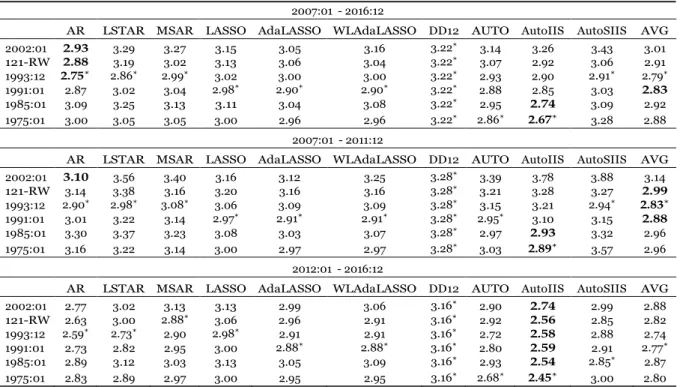
This work evaluates the performance of forecasts using samples of different lengths from the Brazilian Industrial Production Index. Given the volatile and asymmetric nature of the investigated variable, it is also of interest to compare forecasts accrued from nonlinear methods with those of a standard benchmark methods. Therefore, we make two forecasting exercises. One compares, for each method, forecasts using chained series, extended to different starting periods, with forecasts using the latest PIM-PF series available, beginning in 2002:01. The other compares, for each sample, forecasts of different methods with those of AR(p).
−
it
| |
Forecasts are made one-step ahead, re-specifying and re-estimating the models at each step. The AR and STAR models order p is selected by the BIC. To specify the MSAR model, at each forecast step, we estimate 27 different models (1 to 13 lags with switching autoregressive parameters, 1 to 13 lags with fixed autoregressive parameters, and one only with intercept, all with two regimes and including switching intercept and variance) selecting that with the lowest BIC. LASSO, AdaLASSO, WLAdaLASSO and Autometrics algorithms are reapplied at every step. For all methods, a maximum lag order of 13 is considered. In Autometrics, we use a standard p-value of 0.01 for significance tests and saturations of impulse and step indicators.
Since we used a twelve month difference to treat the data, we will suppose E[∆∆12yt] = 0
instead of E[∆2yt] = 0 in the double difference device and denote it DD12, i.e., the industrial
production growth with respect to the same month of the previous year do not continuously accelerate. This modication is straightforward and the interpretation is not impaired.
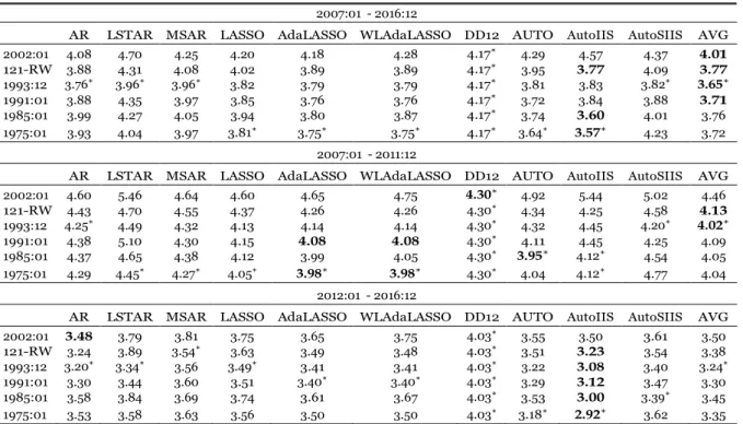
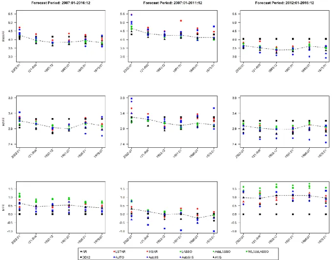
We analyze the forecast horizon starting in January 2007 and ending in December 2016, comprising a total of 120 months, in which forecasts are made one-step ahead. We also an- alyze the forecast performance in both halves of the forecast horizon, i.e., 2007:01-2011:12
and 2012:01-2016:12, in which the first half is characterized by abrupt changes in the series, reflecting the effects of the subprime crisis in Brazilian industrial production and its sub- sequent recovery, and the second by a less abrupt, but persistent, decline in the industrial activity level.
Results are obtained using the chained series starting in 1975:01, 1985:01 and 1991:01. We also consider forecasts made with a 121 months rolling window and with an extending window with the same initial size, i.e., starting in 1993:1213. Note that these starting periods coincide
with those from the closed series obtained from SIDRA and BCB. Using these samples may help identify if more distant methodological benchmarks contain useful information for forecasting recent values.
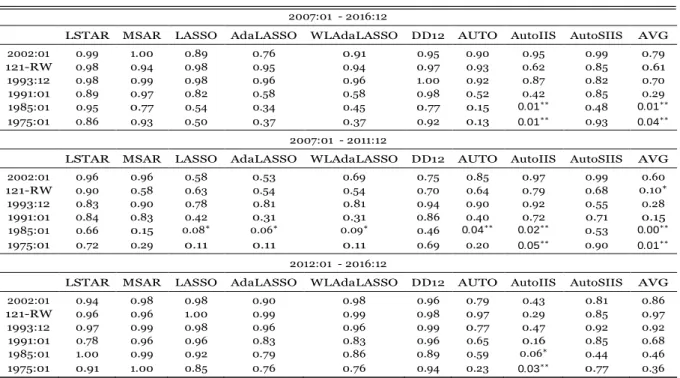
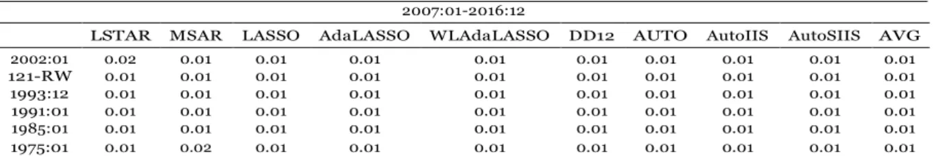
4.3 Forecast Comparison (Diebold and Mariano Test)
To compare the forecasts, we used the Diebold and Mariano (1995) test, which utilizes the forecast errors from two different models to evaluate if one forecast is statistically superior the other.
For the test to be valid, it suffices that assumptions about the forecast errors are valid and it is not necessary to make hypotheses about the models being tested, so that it is possible to compare even predictions that do not come from models.
Let eit be the forecast error from model i in period t and g(eit) some loss function. In this
study, we analyze the results for both g(eit) = e2 , the quadratic loss function, and g(eit) = eit
, the absolute loss function. The key hypotheses are actually made about the difference between the loss function associated with the forecast errors, dt = g(eit) g(ejt). It is assumed
that dt is covariance-stationary:
13These are the starting months of the level series, the annual difference of the index logarithm drops 12